Appendix A2
Basic Optical Interferometers

In addition to the Michelson configuration used in displacement measurements, several other optical interferometers are useful in electro-optical instrumentation. All of them serve the purpose of dividing the beams in a reference and a measurement arm, let the measurand affect the optical path, and recombine the beam to yield the interferometric signal of the type 1+cosΦ at the photodetector.

In this appendix, we will review the properties of basic optical interferometers, namely Michelson, Fabry-Perot, Mach-Zehnder, and Sagnac (Fig.A2-1). All these configurations are basic and can be improved by the addition of extra components or by suitable variants, like exemplified by the Michelson interferometer that becomes the Twyman-Green interferometer when corner cubes are substituted with mirrors (Sect.4.2.1).

A2.1 Configurations And Performances

The Mach-Zehnder interferometer (Fig.A2-1) is used in fiber sensors, and compared to the Michelson, is a sort of unfolded optical interferometer with a second beamsplitter to recombine the propagated beams. It has two separate arms and makes two complementary outputs available. The Fabry-Perot interferometer has no reference path, and interference is between the back-and-forth contributions reflected by the two mirrors. The multipath propagation adds an increased sensitivity compared to the other configurations.

Last, the Sagnac has two counter-propagating beams (clockwise and counterclockwise) in a single propagation path, and is sensitive to non-reciprocal phase shifts only, as it is required in the gyroscope and in magnetic field sensors.

Fig.A2-1 Common optical interferometers and their bulk optics configuration. M and R are the measurand and reference arms, respectively.

Now, let’s consider the signal obtained at the output of the interferometer. In general, the fields returned on the photodetector from the measurement and reference arms can be written in the form of rotating vectors, or E_m =E_m exp i(ωt +ø_m) and E_r=E_r exp i(ωt +ø_r).

The photodetected current is the average of the square modulus of the total field [1], or I_ph=σ(E_m+E_r)², where σ is a conversion factor and the brackets .. denote averaging.

Inserting the fields E_m and E_r in this expression and developing the modulus, we obtain I_ph=σE_m²+E_r²+2E_mE_rRe{expi (ø_m-ø_r} = I_m+I_r+2(I_mI_r)^1/2cos (ø_m-ø_r), where I_m and I_r are the currents produced by the measurement and reference fields, respectively. For I_m≠I_r, we can write the detected current as I_ph=(I_m+I_r){1+[2C^1/2/(1+C)]cos (ø_m-ø_r)}, where C= I_m/I_r is the signal contrast.

Further, by developing the phase term (ø_m-ø_r) in an average part ø_m-ø_r=ø_m-ø_r and a random deviation Δφ, as ø_m--ø_r = φ_m-φ_r+Δφ, the averaged cosine becomes cos (ø_m-ø_r)= μ cos(φ_m-φ_r) [1]. The term μ= cos Δφ has the meaning of the coherence factor of the measurement and reference fields, whereas φ_m-φ_r can be written as Rk(s_m-s_r) in terms of the measurement and reference arm lengths s_m and s_r.

In summary, we may write I_ph in the form:

(A2.1)

where V=2μC^1/2/(1+C) is called the fringe visibility, or contrast factor [5], and R is the responsivity (or response factor) of the interferometer.

Ideally, we should have V=1, but if the coherence factor μ is not unity, polarization is not matched, the beam powers are unequal (C<1) or some stray light is collected, V<1. The factor V is also called the contrast factor because it is coincident with the difference divided by the sum of the maximum and minimum signal amplitudes:

V = (I_phMAX - I_phMIN)/(I_phMAX+I_phMIN)

The responsivity R is a measure of the interferometer’s ability to supply a relative variation of the photocurrent I_ph to a variation of the optical path length in the measurement arm. In terms of the photocurrent signal, the responsivity is the maximum value of the relative derivative of I_ph with respect to ks when V=1:

R = max_s {(I_phk)^-1 dI_ph/ds}

The reason for this definition is that, given the transfer ratio Φ=dks=HdM for the measurand M, the relative signal variation obtained in the photocurrent is readily found as:

(A2.2)

In the Michelson interferometer, from Eq.4.3 of the text, the responsivity is seen to be:

R = 2

a value that is the simple consequence of the go-and-return path.

By inspection of the scheme in Fig.A2-1, it is easy to see that R=1 for a Mach-Zehnder interferometer. In the Sagnac, we usually find a non-reciprocal dependence on +HM and –HM for the two counter-propagating waves, and thus we take R=2 (see Table A2-1).

In the Michelson, we have two available outputs from PD1 and PD2 (Fig.A2-1), and they are complementary to unity. For V=1 they are written as:

(A2.3)

The two outputs are present also in the Michelson and Sagnac interferometers. Signal I_ph1 is the output from PD in the scheme of Fig.A2-1, while I_ph2 (not shown in Fig.A2-1) could be recovered from the beamsplitter output directed toward the source, if we insert an additional beamsplitter to pick it up.

TABLE A2-1 Comparison of basic optical interferometers

Notes: Michelson and Mach-Zehnder may be operated as either unbalanced or balanced (the latter being of course the preferred choice). The Michelson and the Fabry-Perot can have source and detector on the same side if the output is taken by a beamsplitter added on the input path (Fig.A2-1). Responsivity is R=2 for the Sagnac, assuming equal and opposite effects on the two counter-propagating waves. Retro-reflection is for the basic configuration with mirrors; using corner cubes, it is avoided in the Michelson.

Lastly, in the Fabry-Perot, the photocurrent detected at either the front or rear mirror has a dependence of the type:

(A2.4)

where F=2R^1/2/(1-R) is the finesse of the Fabry-Perot resonator and R is the mirror (power) reflectivity [2-4]. Looking for the maximum of the relative slope d(I_ph/I_ph0)/dks in Eq.A2.4, one can find that the responsivity of the Fabry-Perot is just equal to F.

Derivation of Eq.(A2.4).

Let R₁ and R₂ be the (power) reflectivity of M1 and M2, and A=exp-α2s the (power) attenuation suffered in the cavity of length 2s.

Just beyond the first mirror M1, the cavity field E_cav is the sum of two terms: one coming from the input field E₀ and transmitted with through M1, and one coming after the round-trip of the cavity, with reflectance (R₁R₂)^1/2 attenuation A and delay 2ks. Thus, we can write +E_cav A(R₁R₂)^1/2 exp i2ks.

Solving for E_cav, we get:

(A2.5)

Both the outputs from M1 and M2 are proportional to E_cav and we can write them as:

E_M1 = E_cav A [exp i2ks] , and

Therefore, the outputs have the same selectivity, versus ks or λ, as the cavity field E_cav, and we can limit ourselves to study just E_cav.

By taking the square modulus of the field, we obtain the power. Letting R²=A²R₁R₂, the power in the cavity is:

(A2.6)

where P₀ is the incident power, and the last passage is obtained by noting that cos2ks =1-2sin²ks. The output powers from the mirrors M1 and M2 are found as:

P_M1/P₀ = 4 A² R₁ R₂ sin²ks / [(1- R)² +4Rsin²ks], and

P_M2/P₀ = (1-R₁)(1- R₂)A / [(1- R)² +4Rsin²ks]

The diagram of P_cav/P₀ is shown in Fig.A2-2. It has a periodicity 2π in the argument 2ks, or it exhibits periodic resonance at 2(2π/λ)s=N2π or at s=Nλ/2 (that is, at multiples of half-wavelength).

In frequency, the periodicity of resonance Δυ=υ_N+1-υ_N is obtained by letting 2(2πυ/c)s =N2π, and it reads: Δυ=c/2s. For 2ks=N2π, the resonance has a peak value P_cav/P₀=(1-R₁)/(1-R)², even larger than one because of the buildup of power in the resonator cavity, while off-resonance the response has a minimum at 2ks=π, where it is P_out/P₀=(1-R₁)/(1+R)².

The half-width of the resonance curve is calculated from the condition: P_cav/P₀=1/2[P_cav/P₀]_peak, which from Eq.A2.6, becomes (1-R)²=4Rsin²ks and is solved as .

In frequency, the half-height line width is: .

Last, an important parameter of the Fabry-Perot is the finesse [2], defined as the ratio of half-height line width to period, or F=(2/π)Δυ/Δυ_HW.

From the above results, the finesse is given by F=2 R^1/2/(1-R).

Thus, we may substitute F for the factor at the denominator of Eq.A2.6 to obtain the more elegant expression Eq.A2-4.

Fig.A2-2 The response of the Fabry-Perot is periodic by 2π in phase shift 2ks, or by c/2s in frequency. The selectivity is F (=finesse) times better than in other interferometers with a cosine-type response (dotted line)

When using interferometers, further details relevant to performance are the following [4,5] (see also Table A2-1):

- the availability of a reference path. The reference is very important as it allows compensation of the measurement against external disturbances other than the measurand (e.g., temperature, vibrations, EMI). For compensation, the reference path is laid close to the measurement path but shielded from the measurand so as to collect the same disturbance in both arms. Because of the subtraction in the interferometric process, disturbances are canceled out;

- the number of channels available. Basically, the Mach-Zehnder has two outputs readily available for detection, while the other interferometers have one. By an additional beamsplitter in the path going back to the source, a second channel is made available;

- the position of the detector with respect to the source. It is easier to have both on the same side to accommodate them in a single box;

- the retro-reflection from the optical interferometer into the source. Retro-reflections may severely impair the quality of the emitted field, adding amplitude fluctuations as well as widening the spectral line of the laser, especially in frequency stabilized sources;

- the balanced versus unbalanced paths. If reference and measurement paths are nearly the same, requirements on the coherence length of the source are alleviated; - the number of beamsplitters and mirrors: this clearly affects the component count and cost of the final optical assembly;

- cascadeability. This feature has to deal with multiple-sensor operation (as in fiberoptic sensors) or when using the optical interferometer as a filter (frequency channel separation in fiberoptic communications).

A last point to mention is alignment of the mirrors. All optical interferometers considered above are intended for operation with a laser source and basically work with a single-mode spatial distribution of the beams. Thus, their mirrors require an angle alignment accuracy within the diffraction limit θ=λ/πw₀ associated with the Gaussian beam spot size w₀, otherwise an incomplete superposition (Sect.4.5.3) and a reduction of fringe visibility will occur. Of course, if we can use a corner cube in place of the mirror, like in the Michelson interferometer, the angular alignment problem is solved (provided that the corner cube dihedral error is <θ).

Stray light suppression may also be of concern in the interferometer operation. When the laser line width is very narrow, an interference filter in front of the detector will usually be effective to suppress light from the environment.

Alternatively, we may use a spatial filter (see Fig.A2-3), consisting of a lens-and-pinhole combination placed in front of the detector. If the pinhole has a radius r and is placed in the focal plane of the lens with focal length F, only the rays contained in an angle θ=r/F can pass through the filter. Because the minimum θ is the diffraction value, this filtering is very effective.

Fig.A2-3 A pinhole objective combination can be used for spatial filtering of the field reaching the photodetector. The acceptance angle is r/F.

A2.2 Choice Of Optical Components

When we move from conceptual schemes with ideal components as presented in the text, to practical implementation with real components, a number of non-idealities need to be taken into accounts, which if overlooked, may impair or severely degrade the performance we expect in principle.

To illustrate the problems that may be encountered, we will briefly discuss some issues concerning the choice of optical components with reference to a Michelson-based laser interferometer where the beamsplitter and the corner cube are the most critical components.

Beamsplitters

A plain glass-flat model of the popular BK7 glass can be used, provided that it has a reasonable flatness and few surface defects. But, unless we need just the R=4-8% reflection obtained at a low-incidence angle (<10°), we shall treat one surface by a single- or multiple-layer reflection coating to get the desired R. Also, as both front and rear surfaces contribute to reflection, we inadvertently have a sort of parasitic Fabry-Perot interferometer inserted in the propagation path. To avoid this effect, in a glass-flat beamsplitter we shall have one surface coated for the intended reflection, and the other be anti-reflection coated (ARC). Alternatively, to get rid of the reflection from the second surface, we may consider using wedge-flat and pellicle beamsplitter versions. As for any optical surface crossed by the wavefront, surface quality of the beamsplitter should be specified at least as λ/4 distortion and 60-40 scratch and dig, as a rule of thumb.

Polarizing beamsplitters

We may either choose from multireflection or birefringent versions. A multireflection cube is based on the reflection property at Brewster’s angle incidence, by which R_//=0 for the polarization parallel to the incidence plane, while R_⊥≈15%(for n=1.5) for the polarization perpendicular to the incidence plane. Adding several layers of alternatively high and low n, we can obtain a reflection R_⊥≈99%, while R_// stays low (typ. R_//<1%). The layers are deposited on the diagonal surface of a square prism, and the input/output surfaces will be treated ARC. A better extinction ratio R_⊥/R_// (up to 10⁵-10⁷) is obtained by birefringent cube polarizing beamsplitters that use calcite as the material of the prisms. The two halves of the cube are cut along properly chosen directions so as to obtain an index of reflection difference at the diagonal surface boundary, adequate for total reflection of one polarization and transmission for the other. Though one prism would suffice for polarization splitting, a pair of them is normally used to compensate for beam deviation, so that one beam is delivered parallel to the input and the other is about perpendicular. Several cube versions are available under the name of Glan, Glan-Thomson, Wollaston, Nicol, etc.

We can use a polarizer beamsplitter also as a polarizer, but if we only need to select a (linear) polarization state while blocking the other, we may prefer cheaper dichroic-sheet polarizers. Discovered by Kodak’s researchers and widespread in applications [5], these sheets offer a reasonable extinction ratio (typically 10²-10³) in the visible and near infrared, which is often adequate for the use in front of the photodetector.

Corner cubes and retro-reflectors

These components can be understood by starting from the in-plane version of the 90° prism (Fig.A2-4). If the vertex angle is β, the angular deviation between the incident and reflected rays is easily found to be 2β, or 180° for a 90° prism. Incidentally, this general rule is exploited in the pentaprism, which has a vertex angle of 45° and deflects the beam of exactly 90° (Fig.A2-4). The angular deviation is irrespective of the incidence angle α, provided α is within an acceptance angle α_max determined by the total reflection angle internal to the cube. However, working with collimated beams, like in interferometry, even small α_max values (e.g., 5 to 15°) are adequate.

To extend the concept in three dimensions, we need two dihedrals, or the corner cube structure depicted in Fig.A2-4, bottom, in which three reflections are used to deflect the incident beam in two orthogonal planes.

Fig.A2-4 Retro-reflection in a 90° prism and in a pentaprism with a 45° vertex angle (top), and in a corner cube retro-reflector (bottom)

Basically, we have solid-glass and hollow versions of corner cubes.

A solid-glass corner cube (as shown in Fig.A2-4) has an ARC front surface and may reach a reflection efficiency of 95% or better. The points of concern are (i) the fragility of the sharp edges and vertex, easily damaged even during handling of the device; and (ii) the polarization state change that radiation undergoes because of the phase shift at total internal reflection. Because of this effect, for an input linear state of polarization, the output is a mixture of elliptical states, dependent on the cube sector, as shown in Fig.A2-5. This can be disturbing if we rely on the state of polarization for the beam handling in our instrument. However, in a Michelson laser interferometer with two retro-reflectors, if the two corner cubes have the same edge orientation, the beams superpose on the photodetector with the same state of polarization in different sectors, and fringe visibility is unity.

Fig.A2-5 Output polarization in a corner cube for an input linear polarization state

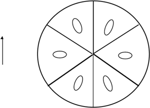
To make the corner cube less sensitive to polarization and protect the total reflection surfaces, these may be metallized (with a thin Au or Al film) and covered by a protection coating. Metallization slightly decreases reflection efficiency (to 90% typically), but increases the field-of-view or acceptance of the device [6].

Alternatively, we may use a hollow-type corner cube, made by three mirrors mounted in a trihedral arrangement at 90° angles. The hollow corner cube is cheaper and has the same performance as the metallized solid-glass cube, but the stability of dihedral angles (to be kept typically within 1 arcsecond for the useful device’s life) may be questionable because of the demanding mechanical stability.

References

[1] S. Donati, “Photodetectors”, Prentice Hall: Upper Saddle River, NY, 2000, Chapter 8.

[2] B. Rossi, “Optics”, Addison Wesley Publ. Co.: Reading, MT, 1957.

[3] W. Lauterborn, T. Kurz, and M. Wiesenfeld “Coherent Optics”, Springer Verlag: Berlin, 1995.

[4] B.E. Saleh and M.C. Teich, “Fundamentals of Photonics”, J. Wiley and Sons: Chichester, 1991.

[5] M. Francon, “Optical Interferometry”, Academic Press: New York, NY, 1966.

[6] B.H. Billings (editor), “Selected Papers on Polarization”, SPIE Milestone Series, vol. MS 23, SPIE: Bellingham, WA, 1991.