Chapter 5
Speckle-Pattern Instruments

When light from a laser source is shed on a plain surface like a sheet of paper or a white wall, the spot appears granular (Fig.5-1). This appearance is termed speckle pattern and came as a surprise to the first researchers experimenting with lasers.

Indeed, spatial coherence was a predicted feature of the laser beam, and common sense was that a laser spot should look smooth. Actually, the spatial distribution of a mode is smooth, and as such is preserved when the beam impinges on a smooth surface. However, a smooth surface is one with roughness much smaller than wavelength, and only a mirror satisfies this condition.

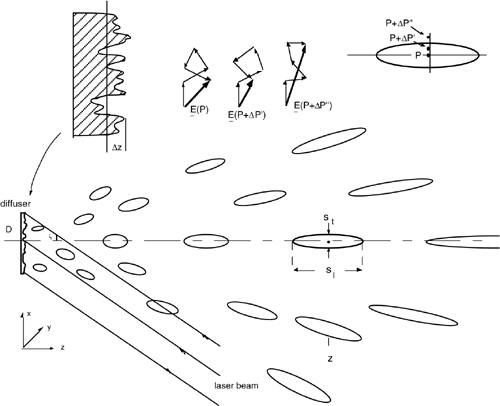
In a normal diffuser or diffusing surface, one with a brightness that looks the same from any line of sight, the vertical scale of roughness Δz=f(x,y), see Fig.5-2, is large compared to wavelength. Each elemental area of the diffuser is then a source of secondary wave leaving the surface with an added random phase φ=2kΔz, replica of the random profile Δz.

The random phase is responsible for destroying the spatial coherence of the near field distribution at the diffuser and for the grainy appearance of the far field.

Fig.5-1 Coherent light projected on a diffusing surface appears granular, and this phenomenon is termed speckle pattern.

In this chapter, we start by considering the statistical properties of the speckle pattern field, first described on a qualitative base and then through a more rigorous analytical approach. We proceed by analyzing the errors of speckle in measurements with interferometers and will conclude with the description of an interferometer imaging technique known as Electronic Speckle Pattern Interferometry (ESPI).

5.1 Speckle Properties

In treating speckle properties, it is customary to assume [1] an ideal diffuser to schematize the statistical properties of surface roughness. As it will be readily appreciated in the following, the ideal diffuser is the model of extreme randomness and gives rise to the so-called fully developed speckle statistics [1]. A real diffusing surface may approach the ideal diffuser rather well, or have a limited randomness of surface roughness that translates itself in a reduced variance. Thus, the ideal diffuser case is the limit case of statistics.

5.1.1 Basic Description

In an ideal diffuser, the height profile Δz=f(x,y) is described by a random function f(x,y). The function is invariant to translations (i.e., properties are the same for all points of the diffuser), has a zero average deviation, Δz=0, and a quadratic mean value or varianc ΔZ² much larger than λ². As a consequence, the phase shift φ introduced by the profile corrugation on diffusion at any point x,y is larger than 2π, or φ=kσ_z >>2π.

In an ideal diffuser, the profile has no spatial correlation on short-scale, or f(x,y) is uncorrelated to f(x’,y’) as soon as |x’-x|and|y’-y|>λ.

This condition can be expressed in terms of the profile correlation function. With the usual

Fig.5-2 Speckle pattern is the field radiated from a diffuser, that is, a surface with roughness larger than wavelength, Δz>>λ (top left). The field at a generic point P is the summation of many individual vectors with a random phase (top center). Moving away from P to P+ΔP’ and P+ΔP’’, the field gradually loses correlation. A speckle grain is a region within which correlation is C≥0.5. Grains are cigar shaped and point to the diffuser center.

definition of the correlation function, that is C_z(Δx,Δy)= ∫ ∫ Δz(x,y) Δz(x+Δx,y+Δy)dxdy, the result expressing spatial uncorrelation is of the type: C_z(x-x’,y-y’) =σ_z² δ(x-x’,y-y’), where δ is the Dirac’s impulse function and σ²_z is the variance defined previously.

Now, let us consider the electrical field E(x,y) leaving the diffuser at z≈0, after illumination from the coherent beam E₁. If we move just a little away from the diffuser, the amplitude E(x,y) is substantially equal to the illuminating one, E₁.

The total phase of E is the sum of a deterministic phase contribution φ₁(x,y)=kx sinξ, due to the incidence angle ξ of the illuminating beam (Fig.5-2) and a random phase term φ(x,y) due to the diffuser roughness.

Because the random phase shift is large, kσ_z>>2π, and has no spatial correlation, the deterministic term is negligible. Therefore, field correlation C_E(x-x’,y-y’) duplicates the statistics of C_z(x-x’,y-y’) or, it is δ-like.

Near the diffuser (z≈0), coherence areas are delta-like regions, and the spatial coherence of the original laser beam is lost, destroyed by the diffuser’s roughness.

Because the δ-like condition holds irrespective of the actual amplitude and phase dependence of the illuminating field E₁ from x,y, we may take for simplicity E₁=const. in the following.

The field E(x,y,z) at any point P in space (Fig.5-2) is evaluated as the vector summation of contributions emitted by all dxdy elemental areas in the source. Each contribution has constant amplitude, but random phase. Such a vector sum is a statistical process known as random walk. The process is the same in all points P of the space, and only the descriptive parameters change with P, not the distributions.

Now, in a generic point P, we write the field as E = E_R+iE_I and recall the results known from statistics about the properties of random-walk process [1-3]. Because of the law of large numbers relative to the addition of many individual contributions, both the real E_R and the imaginary E_I component of the field are normal distributions with zero mean value, E_R= E_I=0. Moreover, the intensity I= E² distribution is found to be a negative exponential. Explicitly, the probability density of intensity is written as p(I)=[1/I] exp -I/I, where I is the average intensity of the speckle field and coincides with the mean square value E² of the field components.

When we move at a substantial distance from the diffuser, the statistical properties remain unchanged, but the δ-like correlation is smeared to a finite-width distribution. In fact, let us go back to point P and consider the field resulting from the addition of elemental vectors with a random phase. Let E(P) be the vector sum, as indicated in Fig.5-2. Now we move to point P’=P+ΔP’. If ΔP’ is small, it is reasonable to expect that the phase of the individual contributions is not so much changed or that E(P+ΔP’) is correlated to E(P). This shall certainly happen, because ab absurdo, if ΔP’→0, E(P+ΔP’) cannot but converge to E(P).

Second, if we move substantially away from P to P’’= P+ΔP’’ and let the deviation ΔP’’ increase, we shall ultimately collect the field contributions with new phase terms, different from the initial ones, whence the resulting vector addition E’’=E(P+ΔP’’) becomes different from the initial result E(P), or, is not correlated to it any more.

Now, the substance is about how large ΔP’ shall be before correlation is lost (or, quantitatively, it becomes less than a specified value, e.g., C<0.5).

This quantity defines the so-called speckle size. The speckles then represent the coherence areas we find at a distance z from an ideal diffuser illuminated with a spatially coherent beam.

In next section, we will calculate the speckle size, both longitudinal (s_l along z) and transversal (s_t along x or y). For a circular diffuser of diameter D, uniformly illuminated, the results are:

(5.1)

As can be seen in Fig.5-2 and from Eq.5-1, speckles are cigar shaped, with the longitudinal size larger than the transversal, and become more elongated as we move away from the diffuser. Speckles point to the diffuser center, and the projection of off-axis speckles is equal to the on-axis speckle.

Subjective and Objective Speckles. The previous discussion holds for the free propagation of the diffused field depicted in Fig.5-2. This case is referred to as one generating objective speckles, in the sense that speckles are only dependent on the diffusing object or target. Another case of interest is when an optical element, for example a lens as in Fig.5-3, is interposed between the conjugated image and source planes. This is the case of subjective speckles, so called because then the speckle depends on the observer, too.

We may analyze the optical conjugation of the diffuser (with diameter D) to an image plane by a lens (with diameter D_L and focal F_L) as drawn in Fig.5-3. For ease of notation, let us take z>>F_L so that the distance p from the lens is p=F_L.

Along its diameter, the lens accommodates a number of speckles N= D_L/s_t given by the ratio of lens diameter to speckle transversal size. Explicitly, here we consider N as a ratio of linear size, not of surface.

Fig.5-3 A lens looking at the source collects N speckles and, because of mode invariance, forms N (smaller) speckles inside the image. As the image is conjugated to the source, N virtual speckles appear projected back on the source. This is the subjective speckle pattern.

Because speckles point to the diffuser center, they are each oriented at a different angle and thus come to a different position at the focal (or image) plane, filling there the image of the diffuser. The image has a diameter D(F_L/z) and contains N=D_L/s_t speckles. Then, the diameter of speckles (transversal size s_t(fp)) found in the image at the focal plane is:

(5.2)

This speckle dimension is the same that we get for objective speckle with a diffuser of diameter D_L at distance F_L.

Now, from the focal plane we can see a virtual image of the source, equal to the one in the focal plane multiplied by z/F_L. On the diffuser, the apparent dimension (transversal size s_t(pr)) we see projected is given by:

(5.3)

Eq.5.3 explains why this speckle regime is called subjective: the diameter of speckles seen on the source is dependent on the lens diameter D_L. Moreover, the speckle size is that generated by the lens aperture D_L, not the target aperture. In addition, the longitudinal size of virtual speckle appearing on the diffuser is s_l(pr) = λ(2Z/D_L)².

The effect of subjective speckle can be visualized easily, looking at a laser spot projected on a wall through a pinhole and varying the diameter of it. For a pinhole, you may use your own index finger, closing it fully folded leaving a small aperture in the middle of the skin fold that you can finely adjust.

5.1.2 Statistical Analysis

We can analyze the statistical properties of the speckle-pattern field starting from the Fresnel approximation to diffraction equation (see also Appendix A5).

Let the diffuser be illuminated by a uniform coherent beam in the plane ξ,η. The complex amplitude of the source can be written as E₁(ξ,η)=E₁ exp iφ(ξ,η) rect (ξ,η,D/2), where: E₁ is the constant field amplitude of the illuminating beam, φ(ξ,η)= k Δz(ξ,η) is the random phase function, associated with Δz, Δz(ξ,η) is the surface roughness, and rect (x) is the step function defining the limits of integration, defined as: rect (x)=1 for x=ξ²+η²≤(D/2)², and rect (x)=0 for x=ξ²+η²>(D/2)².

The function φ(ξ,η) has a δ(ξ,η) spatial correlation and a variance such that Each elemental area dξdη contributes with a spherical wave delayed by kr₁₂ to the field collected at point (x,y) in the image.

In the Fresnel approximation, we may assume and r₁₂/z≈1. By summing up all the elemental contributions in dξdη, we have in the image plane x,y at a distance z (Fig.A5-1):

(5.4)

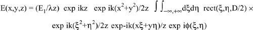
At the right hand side of this equation, after the amplitude E₁/λz the first term is the phase shift of propagation down the distance z, and the second is the field curvature term. Then, we find the integral with the boundary truncation term (rect). The fourth term is again a field curvature term, the fifth is the mixed-coordinate term originating the Fourier transform kernel, and the last term is the diffuser random-phase term.

As a first property we can deduce from Eq.5.4, the field E is a complex quantity with a real E_R and an imaginary E_I part. Both of them are affected by the random part of the phase φ(ξ,η), as it can be seen by developing the exponential under the integration exp iφ(ξ,η)= cosφ(ξ,η) +i sinφ(ξ,η). As φ= kΔz, >>2π, we have cosφ=sinφ=0 and, as a consequence:

(5.5)

Thus, the speckle field has zero-average real and imaginary parts at all points in space.

Second, in the Δz profile, the number of scatterers is very large and, therefore, in view of the central-limit theorem [3], Δz obeys a normal (or Gauss) distribution. At the same way, φ=kΔz and its sine and cosine functions are normal distributions, too.

It is then not surprising that, after linear operations as those performed through the integration in Eq.5.4, the real and imaginary parts of the field, E=E_R+iE_I are both normal distributed and uncorrelated. Accordingly, their probability distributions can be written as:

(5.6)

In Eq.5.6, we have used Eq.5.5 and indicated with the variance of the field components that shall be the same for both E_R and E_I for symmetry reasons. Writing the variance as the mean of squares reveals that it is coincident to the mean intensity:

(5.7)

Another quantity of interest is the field amplitude By transformation of the variables it is easily found that |E| is Rayleigh distributed, or it can be written as:

(5.6’)

About the intensity , knowing that both E_R and E_I are normal distributions and using the rules of variables transformation [3], the probability density p(I) easily follows (see below) as:

(5.8)

Because of the negative exponential distribution, weak (or dark) speckles are more probable than intense (or bright) ones. For example, 10% of speckles have ≤10% the average intensity, 1% have ≤1% the average intensity, and so on.

This is just amplitude fading, a feature hampering measurements that we shall appropriately tackle in all systems working on a diffusing surface rather than a mirror.

Last, the phase of the electric field at a given point P is a random distribution with no information on the initial distance-related phase kz. Computing the phase as φ= atan E_I/E_R gives as a result a uniform distribution of phase on 0-2π as:

(5.8’)

Recall on the change of variables. We want to find the probability distribution p(E) of a random variable E=f(I) related to another variable I, whose probability distribution p(I) is given. We equate the differential probability dp around I and E by writing dp= p(E)dE= p(I)dI. The desired p(E) is then found as: p(E)=p(I)dI/dE= p(I)/[df(I)/dI]. For example, let exp-I/I₀. As df(I) , then p(|E|)=I₀^-1 2|E|exp -|E|², which is the Rayleigh distribution following from the exponential. For joint distributions, p(I,θ)=f(A₁,A₂), the generalization of the method is p(I,θ)=p(A₁,A₂)|J|, where |J| is the Jacobian determinant of the variable transformation, from A₁ and A₂ to I and θ [2].

A summary of the statistical properties of the speckle pattern is reported in Fig.5-4.

The quantities described so far are the first-order statistical properties of the speckle pattern, because they are related to the field in a specific point P. Further information is gathered with the bivariate or joint probability function, which relates the statistical properties of the speckle in two points in space, for example P and P+ΔP in Fig.5-4. The starting point for analyzing the second-order statistical properties of the speckle is the joint probability of intensity and phase in two points P₁ and P₂. This is written as [1,3]:

(5.9)

In this equation, μ exp iψ=μ_c is the complex coherence factor for the field at points P₁ and P₂. The complex coherence factor is defined as the ratio of the mutual intensity normalized to the product of rms values of fields at points P₁ and P₂, or:

(5.10)

where .. indicates the operation of ensemble average on the speckle set, and * is the complex conjugate. The coherence factor μ_c has a modulus μ that may go from 0 (complete uncorrelation) to 1 (full correlation). It is complex because, simply, E(P₂) may be delayed respect to E(P₁) and then ψ=ks(P₂-P₁), where s(..) is the distance between P₂ and P₁.

The numerator in Eq.5.10 is the correlation of the field, which is also called mutual intensity by some Authors [1]:

(5.11)

The correlation has the important physical meaning of a beating signal between the fields at points P₁ and P₂. It is maximum for full correlation, or P₁ approaches P₂, and decreases to zero when fields are uncorrelated, or P₁ moves far away from P_2.. The correlation length is defined as the distance s(P₂-P₁) at which the correlation Cμ has decreased to a specified value (usually 0.5 of the maximum) or has reached the first zero (if Cμ oscillates).

Let us now calculate the speckle size starting from Eq.5.4. To simplify notation, we normalize the field E_st to E₁/λz, and write the integration ∫∫_−∞,+∞dξdη rect(D/2) as ∫∫_rect(ξη,D). With these positions, we have:

(5.12)

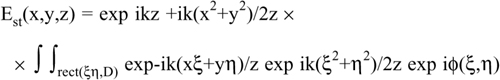
First, we consider the transversal speckle size and write the correlation C_μ for two points with a displacement Δ along x, or:

Fig.5-4 Summary of the speckle pattern statistics: field components E_R and E_I, amplitude IEI, intensity I and phase φ, and joint distribution E₁, E₂

(5.11’)

Inserting Eq.5.12 in this expression, we get:

(5.13)

Here, we have used that, by complex conjugation, the terms in x,y,z have opposite phases and cancel out. Also, the average .., applied to the entire integral at the right-hand side, commutes with the integration and moves into the random-phase terms (the other terms are deterministic).

In view of the uncorrelation from point to point in the source plane, it is:

(5.14)

By substituting Eq.5.14 into Eq.5.13, and recalling that the δ-function has the property of saturating the integration variable, i.e.:

we obtain:

(5.15)

In the last line, the integral expression is recognized as the Fourier transform of the rectangle rect(ξ,ηD/2) of diameter D, calculated in the plane ξ,η and specialized at r=Δ. The multiplying factor is a pure delay, accounting for a phase φ=kΔ(Δ+2x)/2z≈kΔ(x/z). This is the deterministic error we shall expect because of field curvature in an interferometric measurement performed in the speckle regime.

From Appendix A5.3, the integral in Eq.5.15 is readily evaluated as:

(5.16)

and it gives the real part of the correlation we are interested in.

In Eq.5.16, the somb function (bidimensional generalization of the sinc) is the function generating the Airy’s disk (App.A5.3). The somb x drops to half the initial value at x=±0.71, and thus, the speckle size at 50% correlation is s_t = 2Δ = 2x0.71/(D/λz) =1.42 λz/D. If the aperture were square instead of circular, the step function defining the limits of integration would have been rect(x,D/2) rect(y,D/2), and all the previous arguments would still hold, with the final result changed to sinc ΔD/λz. The sinc function drops to half the initial value for x=0.60, whence in this case s_t = 2Δ = 2x0.60/(D/λz) = 1.20 λz/D. These slightly different values show that the factor multiplying the λz/D dependence is close to unity.

In conclusion, we simply take as reference value for the transversal size:

(5.17)

Second, we can repeat the calculation for the longitudinal size. Let us consider a displacement Δ along z and write the correlation as E_st(x,y,z+Δ)E_st*(x,y,z)

Writing Eq.5.12 for this case yields:

(5.18)

Also in this case the first term multiplying the integral is a pure phase term φ. This phase φ includes the expected (and correct) delay kΔ= k[(z+D)-z] as well as the curvature (deterministic) error kΔ(x²+y²)/2z², which is small with respect to kΔ but will show up when we perform an interferometric measurement in the speckle regime.

The term given by the integral is real and, using Eq.A5.5, is given by:

(5.19)

As for the transversal dimension, we have a somb function for the correlation of the field. The somb x drops to half the initial value at x=±0.71, and thus, the speckle size at 50% correlation is: s_t = 2Δ = 2x0.71/(D²/4λz²) =1.42 4λz²/D². If the aperture were square, the result would change to sinc ΔD²/2λz², whence s_t =2Δ =2x0.60/(D²/4λz²) =1.20 4λz²/D² in this case. In conclusion, we can take as reference value for the longitudinal size:

(5.20)

5.1.3 Speckle Size from Acceptance

In previous section, the transversal and longitudinal sizes of the speckle were calculated on the base of correlation width of the field. Correlation is tightly related to coherence, and we may interpret s_l and s_t as the coherence lengths (along longitudinal and transversal directions) and the speckle grain as a coherence region, or a mode of the field.

This interpretation is indeed correct, and in this section we show that speckle size can be traced to the size of the spatial mode found at a distance z from a diffuser.

A theorem on the invariants of radiometry (Ref.[5], App.A2.3) states that the acceptance a of an aperture receiving power under a solid angle Ω and on an area A is equal to N times λ², or:

(5.21)

where N has the meaning of number of modes, or of degree of freedom associated with the area-solid angle aperture.

Let us apply this theorem to the speckle propagation, with reference to Fig.5-5. We let N=1 for a single mode, and note that radiation is received at distance z under the solid angle Ω=π(D/2z)². The receiving area associated with a (transversal) spatial mode of width s_t is A=π(s_t/2)². Inserting in Eq.5.21, we get λ²= π(s_t/2)²π(D/2z)² whence s_t=(4/π)λz/D.

Second, the bundle of rays in the solid angle Ω keeps limited transversally to an extent ≤s_t (Fig.5-5) for a longitudinal width s_t/θ, where θ=D/2z is the angular aperture of the bundle. Combining these expressions gives s_l=(2/π)λ(2z/D)² as the longitudinal size. A comparison with Eq.5.1 shows that these values are the same already found, except for a minor multiplying factor of the order of unity.

Fig.5-5 Geometry for the calculation of speckle size as a spatial mode

5.1.4 Joint Distributions of Speckle Statistics

The joint statistics of the speckle pattern describes the properties of the field in two points P₁=P and P₂=P+ΔP in space (Fig.5-4). When ΔP is comparable with the speckle size, the joint statistics gives relative-amplitude and phase-difference information important to displacement and vibration measurements made with interferometers on diffuser like target surfaces.

The starting point is the joint probability density of intensities and phases p(I₁,I₂,φ₁,φ₂) given by Eq.5.9. This probability is a direct consequence of the Fresnel diffraction integral and of the diffuser surface randomness.

We can get the joint probability density of intensities p(I₁,I₂) by a double integration of Eq.5.9 on φ₁ and φ₂ from 0 to 2π. In this way, we obtain [1,3,6]:

(5.22)

In this equation, ℑ_o is the modified Bessel’s function of first kind, zero order, μ is the modulus of the coherence factor (Eq.5.10), and σ² is the variance of the (real and imaginary) field components (Eq.5.7). About this variance, we may recall that it is also 2σ²=I₁=I₂. Similarly, the joint probability density of phases p(φ₁,φ₂) is obtained by a double integration of Eq.5.9 on I₁ and I₂ from 0 to ∞, and the result is [3,6]:

(5.22’)

Here, β=μcos(φ₁-φ₂-ψ), and ψ is the argument of the complex coherence factor μ_c=μexp iψ. The probability p(φ₁,φ₂) is brought to the probability density of the phase difference φ₁-φ₂ by changing the variables σ₁,φ₂ in their sum and difference and integrating on the sum. This gives as a result p(φ₁-φ₂)=2πp(φ₁,φ₂).

The joint probability p(φ₁-φ₂) is plotted in Fig.5-6 as a function of φ=φ₁-φ₂-ψ and with the coherence factor μ as a parameter. In the diagram, we start at μ=0 with the uniform distribution p=1/2π. As μ increases, the probability density becomes more and more peaked around φ=0, up to the limit case μ=1 (not shown in Fig.5-6) when it becomes a Dirac delta, p(φ₁-φ₂)=δ(φ₁-φ₂).

Fig.5-6 Probability density p(φ₁-φ₂) of the phase difference plotted for some values of μ, the modulus of the coherence factor.

From the probability density, we can calculate the variance σ_φ² of the phase difference φ₁-φ₂, that is, the error in a phase measurement performed in the speckle regime between two points with a coherence factor μ.

As it is φ₁-φ₂=0, the variance is given by where we have let φ=φ₁-φ₂. Collecting the terms and using Eq.5.22’, one is left with the evaluation of an integral that appears intractable at first sight, but is finally solved with the result [6]:

(5.23)

Let us now deal with conditional probabilities. They are useful to consider when we can add any knowledge of one of the variables (I₁,I₂,φ₁,φ₂), or combination of them. Taking account of this knowledge, we may restrict the set of speckle realization to the subset of conditioned values and be able to obtain a smaller variance or measurement uncertainty.

For example, let us assume that the intensity I₁ in point P₁ is known, and we want to compute the probability of intensity at point P₂.

The conditional probability p(I₂|I₁) of having I₂, once I₁ is known, is given by Bayes’ theorem [2] as the ratio of the joint probability to the probability density of the conditioning variable:

(5.24)

Combining Eqs.5.24 and 5.22 we obtain [6]:

(5.25)

We can now calculate the first and second moments of this distribution, that is:

(5.26)

and obtain the conditioned mean and variance of intensity, that is:

(5.27)

Fig.5-7 Mean value (left) and variance (right) of intensity I₂ conditioned to I₁, as a function of μ, and for some values of the intensity I₁ as a parameter. The ‘free’ values of mean and variance of the unconditioned distribution are also indicated.

In Fig.5-7 we report the diagrams of mean and variance of intensity I₁ conditioned to intensity I₂ versus the modulus of the coherence factor. The mean value is standardized to I₁=I₂=2σ² and the variance to σ², the ‘free’ value. From Fig.5-7 we can see that when the conditioning intensity I₁ is larger (smaller) than the mean, also I₂ is, on the average.

The variance for large conditioning intensity I₁ is larger than the ‘free’ value, but not so much larger. For example, I₁=5I gives only σ_I2²≈1.60σ² (at μ≈0.6), or a relative standard deviation σ₁₂/I₁≈0.25. Of course, if we move to the high-correlation region μ≈1, this relative standard deviation is even smaller.

In summary, a bright speckle has comparatively less intensity noise.

Another conditioned probability is that of intensity I₂, when we know both intensity I₁ and phase φ₁ in the other point. This probability can be computed starting from Eq.5.9, and the result is given in [6]. Using the definitions (Eq.5.26), mean and variance are found as:

(5.28)

In Eq.5.28, erf is the standard error function [2] and we have let and .

Mean and variance of the intensity are plotted in Fig.5-8 for some values of the conditioning parameter I₁cos²φ, the projection of intensity I₁ on I₂, being φ=φ₂-φ₁ as usual. The abscissa variable is the modulus of the coherence factor extended to negative values by the multiplication to the sign of cos φ to account for anti-correlation when φ≈π

As we can see from Fig.5-8, similar to intensity, also the phase becomes more regular in correspondence to bright speckles.

Last, we want to compute the conditional probability density of phase φ₂, with the intensities I₁ and I₂ and the phase φ₁ as conditioning variables. Before proceeding, let us remark that, if phase φ₁ is known, then the phase difference φ=φ₂-φ₁ is the only statistical variable of significance.

Fig.5-8 Mean value (left) and variance (right) of intensity I₂ conditioned to I₁ and to the phase difference φ, as a function of the coherence factor and for some values of the projected intensity I₁cos²φ as a parameter.

Fig.5-9 Variance of the phase difference σ_φ² 2 normalized to π²/3, as a function of the coherence factor μ, and of the dynamic range factor μ=1-ζ² (right), with the relative intensity (I₁I₂)/<I> as a parameter. The ‘free’ variance given by Eq.5.23 is also plotted for comparison. The right hand diagram is an expansion near μ=1, the region of high coherence, and is plotted for μ=1-ζ².

Incidentally, the phase difference is just the quantity we are interested in for a measurement of optical path length. Thus, we consider the conditional probability p(φ|I₂,I₁). As before, by integration of Eq.5.9, we find [6]:

(5.29)

Because of the same symmetry of Eq.5.22’, the mean value of phase φ|_I2,I1 is still given by the ‘free’ value of Eq.5.23, for which the diagram is plotted in the left-hand part of Fig.5-9. The variance σ_φ²|_I2,I1 follows from the definition (Eq.5.26) and is found as:

(5.30)

In Eq.5.30, we have let z=μ(I₁I₂)^1/2/σ²(1-μ²), and ℑ_n is the n-th order modified Bessel function of the first kind (usually denoted with I_n).

Fig.5-9 (left) shows the probability density of phase conditioned to intensity against the coherence factor μ Also plotted is the ‘free’ value of phase variance, given by Eq.5.23, and relative to the full set of speckle realization. We can see from the diagram that the free value decreases from π²/3 to zero as μ varies from 0 to 1. The conditioned variance is always smaller than the free variance for (I₁I₂)/I>1, that is, where the speckle is locally more intense than the average. The decrease of variance—and of measurement error—is particularly sizeable near μ≈1 where the speckle field keeps well correlated.

Equations 5.23 and 5.30 become indeterminate forms when μ→1, and cannot be used directly in the region of high coherence. Then, we let μ=1-ζ² and obtain the following asymptotic behavior for small ζ:

(5.23’)

(5.30’)

The main dependence of both free and conditioned phase variances is on ζ². The multiplying factor steadily increases for ζ→0 for the former and is given by the inverse of the relative speckle intensity (I₁I₂)/I for the latter. The ratio of rms phase error σ_φ to dynamic range factor:

(5.31)

is plotted versus ζ in Fig.5-9 (right).

5.1.5 Speckle Phase Errors

Let us now evaluate, from the results of speckle pattern statistics found in previous section, the noise-equivalent-displacement (NED) associated with the interferometric measurement. Let the phase measured on a displacement z₂-z₁ be φ=k(z₂-z₁), where k=2π/λ, and the error superposed be σ_φ. Then, we may recall from Sections 4.4.1 and 4.4.7 that the NED can be written as:

(5.32)

where the second equation follow from the definition of Eq.5.31.

The factor ζ is found from the coherence factor as μ=1-ζ². For the two cases considered in Section 5.1.2, of longitudinal and transversal displacements from an initial point P to a final point P+Δ, the coherence factor has the expression (see Eqs.5.16 and 5.19):

(5.33)

In the two cases, it was X=ΔD/λz and X=ΔD²/λz². Recalling Eqs.5.17 and 5.20, we may write the factor as X=Δ/λs_t and X= Δ /s_l, s_t and s_l being the transversal and longitudinal size of the speckle. In a generalized form, we can write:

(5.33’)

and s_spckl is the current size for the experiment at hand.

Now, we may develop at the third order of X the somb function and obtain μ as:

(5.34)

By comparing with μ=1-ζ² we get:

(5.34’)

Finally, we go back and insert Eqs.5.33’, 5.34’ into Eq.5.32. The equivalent displacement error due to the speckle turns out to be given by the expressive form:

(5.35)

Eq.5.35 is interpreted as follows. The speckle error, expressed in terms of wavelength (NED/λ), is given at first instance by the ratio of displacement Δ to speckle size s_spckl, either longitudinal or transversal.

The statement is refined by considering the multiplying factor C/42. This factor is not too far from unity and depends on the modality of measurement (that is, a free speckle statistics versus a conditional statistics), as indicated in Fig.5-9 (right).

5.1.6 Speckle Errors Due to Target Movement

The treatment considered so far holds for a displacement of the observation point in the speckle field. That is, it describes the error made by moving the observer from an initial point P to a final point P+Δ in the speckle field (Fig.5-2), while the diffusing target is still.

A different and more frequent case is that of a still observer and a moving target. The target movement may be either transversal or longitudinal, as shown in Fig.5-10. For both movements, we assume that the illumination beam does not move (this is the actual reference frame). Then, the illumination on the target is unaltered in a longitudinal movement, whereas the target sample illuminated by the beam changes in a transversal movement.

We can calculate the correlation function C_μ= E(P)E*(P+Δ) along the steps that lead to Eqs.5.16 and 5.20. In particular, for a transversal displacement Δ of the target, we shall change ξ to ξ+Δ in all terms of Eq.5.12, whereas, for a longitudinal displacement Δ, we shall change z into z+Δ.

By repeating the calculations carried out in Sect.5.1.2, we obtain in either case the same result that reads E(P)E*(P+Δ)=somb(Δ/s_spckl), in which s_spckl is the longitudinal (or transversal) size of the field projected by the target.

Thus, it is like the target drags along its speckle field when it moves with respect to the laser beam of illumination (Fig.5-9). Therefore, Eqs.5.22 to 5.35 apply also to interferometric measurement on a moving target and give the error caused by the speckle regime.

Fig.5-10 A moving target drags the speckle pattern field projected on the measuring system (for longitudinal displacement as shown here, the field is dragged along Δz). The correlation lengths for transversal Δx and Δz displacements are coincident to the speckle sizes s_t and s_l.

5.1.7 Speckle Errors Due to Beam Movement

Another case of concern is the movement of the illuminating beam on the target, when all other parts are still. The movement is not intentional, usually, but may be imparted to the beam by wandering and turbulence effects (App.A3.2) especially when operation is on a sizeable path length (say L>50 m).

We can treat this case by calculating the correlation function C_μ= E(P)E*(P+Δ) when the diffuser coordinate ξ is changed to ξ+Δ Again by the calculations carried out in Sect.5.1.2, we obtain in this case the result E(P)E*(P+Δ)=somb(Δ/s_t), where s_t is the transversal speckle size of the field projected by the target. This result is intuitive and confirms that moving the target is equivalent to moving the illuminating spot on it.

5.1.8 Speckle Errors with a Focusing Lens

We may use an objective lens to focus the illuminating beam onto the target, as illustrated in Fig.4-16 and generally used in laser vibrometer (Sect.4.6).

To treat this case, we shall just recall the results of Sect.5.1.1 about subjective speckle. At the focal plane of the objective lens, the transversal and longitudinal size of the speckles are given by (Eqs.5.2 and 5.3):

(5.36)

The parameters governing the speckle size are the lens focal length F_L and diameter D_L.

At the object plane, because of the optical conjugation provided by the objective lens, the speckles are seen stamped on the target with apparent dimensions:

(5.37)

Eq.5.37 tells us that, when a lens is used, the aperture governing the speckle dimension is the lens diameter, not the target size.

5.1.9 Phase and Speckle Errors Due to Detector Size

In all interferometers, after the beam recombination we end up with a photodetector that provides the signal carrying the path length information. Let us now consider the effect of finite detector size on (i) the speckle error, a random contribution, and (ii) the field curvature error, a deterministic phase error.

Let us first consider the speckle statistics versus detector diameter D_det. In the image plane of the focussing lens (Fig.5-3), if the detector is smaller than the speckle size D_det≤s_t(fp)=λF_L/D_L, we can assume that the speckle distribution is point-wise sampled. Then, the results of preceding sections directly apply.

A small detector delivers a small signal, however. We might increase the detector size so that it collects N_sp=(D_det/s_t(fp)² speckles. In this case, what about the statistics?

Integration of the received field on several speckles can be treated as the sum of independent samples of the same statistical ensemble. We can consider two cases:

- incoherent addition of speckles intensity when we perform a (normal) direct detection,

- coherent detection of the speckle field when we add a local oscillator or reference beam on the detector (see also Sect.8.1 of Ref.[5]) with the aim of performing a phase measurement.

In the case of incoherent addition, the sum of N_sp speckles gives N_sp times the intensity I of the single speckle, as an average. The probability of the sum of N terms p_N(I) is the convolution of the single p(I), repeated N times, or p(I)* p(I)*… *p(I). For the exponential distribution p(I)=<I>^-1exp–I/<I>, we get [2,4] the result p_N(I) = (I/<I>)^N(N!)¹exp–I/<I>. Thus, small amplitude speckles are no more the most probable, and for large N we go to the well-known result of the central-limit theorem [2]. This is a Gaussian (or normal) distribution of intensity with a relative standard deviation equal to 1/N.

In the case of coherent detection, we have to deal with the sum of N independent field components E, each with a normal distribution p(E) (Eq.5.6) having zero mean value and σ²=<I> variance. The sum of such contributions is again the convolution of the single p(E), repeated N times, or p_N(E)= p(E)* p(E)* … *p(E). The resulting distribution p_N(E) is still normal, with a mean value and a variance both equal to N times the mean and variance of the single p(E). Thus, the mean value of the sum remains zero, while the variance is increased to Nσ².

Considering the readout configuration of interferometers (Sect.4.5), the external configuration can even use a large area photodetector, and the previous arguments are fully applicable. On the contrary, the self-mixing configuration has an acceptance determined by the laser cavity aperture, receiving the retro-reflected wave.

This acceptance is λ² or, in other words, the equivalent area of the detector is that of the single mode. Therefore, to use a self-mixing configuration in the speckle regime, we shall match the spatial mode of the laser to the speckle transversal size.

Second, let us consider the deterministic phase error given by field curvature. This is caused by the term exp ik(x²+y²)/2z that, in Eq.5.4, multiplies the correct phase term exp ikz due to propagation. As the detector coordinates x,y have a radial extension from r=(x²+y²)=0 to D_det/2, we integrate to field exp ikr²/2z on 2πr dr and average on the area πD_det²/4. Thus, we obtain the field collected by the detector as:

(5.38)

The phase is contained in by the exponential term of Eq.5.38 as φ= k(D_det/4)²/z. The sinc function is close to unity in the reasonable assumption of a small detector, D_detλz, and can be dropped.

The phase φ term adds to the correct phase kz of the propagation (term exp ikz in Eq.5.4), and thus we have a deterministic (or systematic) error. We may translate this error in an Equivalent Displacement Error (EDE) letting EDE=φ/k, and we get from Eq.5.38 EDE =(D_det/4)²/z. Last, if our measurement goes from distance z₁ to distance z₂, the error is EDE=(z₂-z₁)(D_det/4)²/z₂z₁. With a reasonably small detector, for example D_det= 1mm, the error is small on a wide range, say, z₁=100mm to z₂=500mm. In this case, we get: EDE= 400(1/4)²/100.500mm =0.5μm. However, if it were D_det=4mm, z₁=50mm, z₂=100mm, the error would be serious, EDE=10 μm.

5.2 Speckle In Single-Point Interferometers

With regard to operation of interferometers on diffusing surfaces, we have already outlined several topics in Chapter 4, that consider the extension of the basic interferometer (Sect.4.2.3.4), speckle–related errors (Sect.4.4.7), and vibrometers (Sect.4.6). Here, we treat the effect of speckle statistics in vibration and displacement measurements made with interferometers. By vibration we mean the small amplitude range (less than ≈100 μm), and with displacement we mean the range of large amplitudes (>0.1 mm).

Our aim is to keep the speckle effects under control, starting from the easy task of detecting small-amplitude displacements, and then trying to extend operation on large displacements as required in machine-tool control.

5.2.1 Speckle Regime in Vibration Measurements

The first consequence of the speckle statistics is amplitude fading. In fact, the intensity of the speckle pattern field is distributed as a negative exponential (Eq.5.8). Then, in a vibrometer aimed to a target, it will be not so unlikely that we fall on a weak or dark speckle, with the intensity I substantially smaller than the average value I.

Because of the negative exponential, the probability to get I<0.1I is p=0.1, that of I<0.01I is p=0.01 and so on. This is amplitude fading because in a small, but not negligible, fraction η of cases, the signal returning from the target will be smaller than ηI. No matter how sensitive or low threshold the signal-processing circuits are, we cannot avoid falling below the minimum signal condition.

There are several ways to get around the amplitude fading. First we may incorporate in our instrument a circuit sorting the intensity level and warning the operator when the speckle intensity is too small. The operator will then move a little bit the laser beam projected on the target to another spot. Thus, we fall on another realization of the speckle statistics, and this can be a normal or even luckily an intense speckle, with I>I and a good conditional statistics (see Eq.5.30’).

The second approach uses an Automatic Gain Control (AGC) to restore the signal amplitude so that it is adequate for circuit levels. Of course, if M is the dynamic range improvement of the AGC, the threshold of signal loss is moved to a lower value, ηI/M, but not eliminated.

A third strategy is exploiting sensor duplication, a technique usefully employed in radio engineering and known as diversity. We use two receivers, slightly apart in space, to sample different realization of the speckle statistics. With this, the probability of fading on both signals, below ηI is η², a smaller value than a single channel, yet not zero.

From the point of view of applications, the first strategy is usually quite acceptable for a vibration-detecting instrument. The second and the third can also conveniently be incorporated and reduce the probability of fading down to very acceptable levels.

A fourth possibility, if allowed by the application, is that we can use a superdiffuser as the target surface. A superdiffuser is a piece of back-reflecting tape or varnish of the type used for enhancing the visibility of traffic sign at night. Also known as Scotchlite^TM in a commercial product, the superdiffuser provides a gain of a factor 20 to 50 (typically) in the back-reflected signal reaching the interferometer. However, application of the tape or of a varnish drop on the target is a quasi-invasive operation that cannot be accepted in all circumstances. A final option mostly used in interferometers and described later (Sect.5.2.2) is that of dynamical tracking of a bright speckle, one that at the same time cures fading and phase error.

Another concern is speckle phase error. This error affects the accuracy of the measurement performed on a diffusing surface. The error is usually small, but, as we can go down to measure very minute amplitudes of vibration (Sect.4.6), it may become important as well. As already seen in Sect.5.1.5, the error translates itself in an NED given, in units of wavelength, by the ratio of vibration amplitude Δ to speckle longitudinal size s_l(trg) (Eq.5.35). In a vibrometer, the speckle size can be made much larger than the dynamic range Δ_max (i.e., the maximum amplitude of vibration we want to detect). With s_l(trg)Δ_max, the phase error is made negligible.

As a practical example, assuming the reasonable values λ=1μm, D_L=30mm, and z=300mm, the speckle longitudinal size is s_l(trg)=λ(2z/D_L)²=400μm. The phase error λΔ_max/s_l(trg) is 2.5 nm for a swing of 1μm, is 0.25 μm for a swing of 100 ?m, and so on. Moreover, if we choose a bright speckle, we could be able reduce the phase error further, taking advantage of the factor C<1 in Eq.5.35.

5.2.2 Speckle Regime in Displacement Measurements

In displacement measurements, fading and phase error problems are more serious because we want to span a large dynamic range and cannot make s_l(trg>>Δ_max.

This is the case of application to tool-machine numerical control, calling for displacement from tens of cm to meters. These equipment may employ an optical rule (Ref.[5], Sect.9.3.4) as the least expensive solution, or a multiaxis interferometer equipped with corner cubes (Fig.4-13) for increased performance. The use of a plain diffuser has the advantage of eliminating the problem of cleaning the lens and optical parts.

If we are to measure a large displacement, it is likely that we are compelled to use a digital readout, by counting λ/2- or λ/4-transitions, to develop the several-digit figure. Then, our measurement is incremental and cannot tolerate a count loss. Nor are we allowed to read just the spot moving it away from a dark speckle like in vibrometer. Count loss due to signal fading is the main concern because, when it happens, we are forced to reset the instrument to its mechanical zero. Thus, watching phase errors to be reasonably small, we focus on fading.

Fading shall be counteracted by a combination of the techniques discussed in Sect.5.2.1, including speckle size tailoring, ACG, and detector diversity. A super-diffusing target will be used first if allowed by the application.

As a first issue, we have to choose the beam size. A small beam size gives a large speckle that keeps the phase error small, but the signal collected is small and is affected by quantum noise. A large NA objective lens helps collect a substantial return signal so that the quantum noise is low, but increases the speckle error.

Example of evaluation. We may start requiring a large speckle size. With the external configuration, we shall collimate the laser beam on the full dynamic range Δ_max to be covered. Using Eq.2.4, we get a spot size w=(λΔ_max). Then, the longitudinal speckle size is s_l=λ(2Δ_max/w)² and, inserting the previous expression, turns out as s_l=4Δ_max,. In this way, we are inside a single speckle on the full dynamic range. The signal collected in this last speckle is very weak, however. If P_L is the power leaving the laser, and we use half of it in the reference path, P_L/2π is the intensity at the target, and (P/2π)π(w/Δ_max)² is the power collected by the receiver. The attenuation respect to the power leaving the laser is accordingly (w/Δ_max)²=λ_max. Using λ=1μm and Δ_max=1m, we shall be prepared to a –60 dB loss.

On the other side, if we take a sizeable diameter of the objective lens, let’s say D_L =30mm, in place of the small w (typ.=λΔ_max=1mm), we limit the loss to -30 dB, but are faced with a small speckle dimension, s_l= λ(2Δ_max/D_L)²=4mm only. In a 1-m=Δ_max dynamic range, we would find 250 speckle passages (each with a ≈ λ error each).

Another point to consider is that a practical system should be able to tolerate residual walk-off movement of the target or of the illuminating beam (the corresponding errors are given in Sections 5.1.6-7). To illustrate a reasonable compromise, we take a dynamic range Δ_max=1m, and let n=10 speckle passages in it, so that the error is just 10λ=10μm (or 10^-5) and the average speckle size is s_l=100mm. At λ=1μm, this means that we can use a lens diameter D_L=6-mm in s_l= λ(2Δ_max/D_L)². The chosen speckle size gives room for a reasonable lateral walk off of the target on the Δ_max=1m dynamic range.

As an efficient method to cure fading, let us now consider dynamical tracking of the speckle, a technique that has been recently introduced [7]. The basic idea consists in moving the beam projected on the target to maximize the signal amplitude or, to keep it locked to a bright speckle while the target eventually undergoes its movement. Locking to a bright speckle has two advantages: the probability of fading is greatly reduced, as it will be shown later with experimental results, and the phase statistics improves because we work consistently at a high I/I ratio (Fig.5-9).

The hardware to perform speckle tracking with a self-mixing interferometer configuration is shown in Fig.5-11. We use a pair of microactuators, in the form of two small bars mounted inside the objective lens holder along the X and Y direction. Specifically, the actuators we used are made of lead-zircon-titanate Pb(Zr,Ti)O₃ (PZT) ceramics. By actuating the PZT elements, we generate a (small) lateral displacement Δ of the lens (along X and/or Y), and the incoming beam is deflected by an angle Δ/f, with f being the focal length of the objective lens. On the target located at a distance z, the beam deflection is zΔ/f. In the practical implementation, it suffices to deflect the beam of just ≈5-20μm on the target to follow the local maximum intensity.

Fig.5-11 Arrangement to track the speckle maximum. Two small bars of PZT ceramic are mounted in the lens fixture and move the lens along the X and Y axes, changing the spot position on the target just of a few micrometers (adapted from Ref.[7], by courtesy of IEEE).

To detect the direction of signal increase and actuate the deflection accordingly, we use the well-known method of small signal sensing and phase detection. For example, to track the maximum along X, we feed the X-axis PZT ceramic with a small-amplitude square wave at audio frequency. The photodiode on the laser rear facet detects the signal amplitude, a square wave that will be in-phase or antiphase (shifted by π) with respect to the PZT drive. When we find it in-phase, we will increase the actuator dc drive, whereas, in antiphase, we will decrease it. When we get the maximum, the photodiode signal is at twice the drive frequency. Thus, demodulation of the photodiode signal with the PZT drive square wave, followed by a low-pass filtering (Fig.5-12) provides the required tracking of the maximum, but along X for the moment.

To derive the two X and Y error signals from a single photodiode output, we take advantage that phase and quadrature signals are orthogonal. Indeed, we use the same square wave, with 0° and 90°-phase shift, as the drive of the X and Y actuators. When the photodiode signal is demodulated by the corresponding X and Y waveforms, the contribution from the other channel is not seen because it is dephased by 90° (or, orthogonal).

This concept is called dither of phase tracking and can be implemented as shown in Fig.5-12. With the dither, the optical axis of the laser beam projected out the objective lens is moved along a square path in the X-Y plane. On the target, the side of the square is adjusted to be a few μm, i.e., much less than spot size, yet enough to track the speckle maximum.

In the schematic shown in Fig.5-12, a circuit rectifies the self-mixing signal out from the photodiode and then multiplies it with the two square waves driving the X and Y PZT actuators. After a low-pass filter, the signals are sent to the PZT actuators. As we get a beam movement in the direction of increasing signal for both axes, a final state of equilibrium is reached when both axes are on a local maximum, or a bright speckle.

Fig.5-12 Block scheme of the speckle-tracking circuit. The signal from the photodiode is rectified peak-to-peak and demodulated with respect to the dither frequency, in phase and quadrature. The results are the X and Y error signals that, after a low-pass filtering, are sent to the piezo X and Y actuators to track the maximum amplitude or stay locked on the bright speckle (from Ref.[7], by courtesy of IEEE).

The feedback loop is limited by the response time of the PZT actuators in the range of τ_PZT =0.1-0.3 ms for small (≈2×2mm) bars. This response time is adequate to follow the target movement up to a speed s_l/τ_PZT. For a speckle size of s_l = 100 mm, the target speed we can track without errors is s_l/τ_PZT =0.3-1 m/s.

To illustrate the result obtained by the tracking method, we start considering the statistical distribution of the field amplitude |E|. As given by Eq.5.6’, the ideal diffuser has a Rayleigh-distributed probability density p(|E|) of field amplitude, and this is one of the curves plotted in Fig.5-13 (left, thin line). Also plotted in Fig.5-13 (left, bars) is the experimental result measured on a white paper target (specifically, plain letter paper). To improve the match, a small nonideality of the real diffuser is accounted for. This is done by assuming the target re-diffuses 98% of incoming radiation and reflects (without altering the phase) the remaining 2%. The calculated distribution of field amplitude for such a real diffuser is also shown in Fig.5-13 (left, thick line).

On the abscissa, the field |E| is standardized to the value that makes C=1 in the self-mixing intereferometer configuration. From Eq.4.35, we have , where E₀ is the field leaving the laser. Thus, the field for C=1 is .

Fig. 5-13 Probability density function p(|E|) of the field amplitude |E|, with the amplitude normalized to 1 for a value C=1 of the self-mixing parameter.
Left: Thin line is the Rayleigh distribution for an ideal diffuser, and thick line is the result of a numerical simulation for a real surface, with 2% reflection and 98% diffusion, and fully developed speckle statistics. Bars are experimental data for plain white paper (z=50cm, w_las=2 mm).
Right: With the bright-speckle tracking on, the experimental distribution moves to significantly larger |E| (dark bars) as predicted by simulations, with respect to the circuit-off distribution (gray bars). Adapted from Ref.[7], by courtesy of IEEE.

When the circuit tracking the bright speckle maximum is switched on, the p(|E|) distribution becomes that of the right-hand diagram of Fig.5-13. The improvement of tracking is evident looking at the small-amplitude part of the diagrams. Occurrence of small amplitudes is greatly reduced.

In particular, with the speckle tracking circuit, we can immediately work with the self-mixing configuration of the interferometer, one demanding a given minimum signal amplitude (the condition C≥1) to stay in the up/down switching regime of counts (Sect.4.5.2.5).

The data of Fig.5-13 are relative to a working distance z=50-cm and a laser spot w_las=2-mm on the diffusing target. In this condition, the probability of C<1 (loss of counts) is ≈10% in normal conditions, but drops to 0.5% with the tracking-circuit on.

Thus, we can operate on a substantial span of distance without amplitude fading, even with the self-mixing interferometer, and can expect that the phase error is kept low.

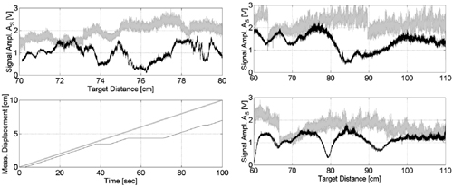
Fig.5-14 Examples of simulations of amplitude (top curves) and phase (bottom curves) of the returning field. The diffusing target moves from 108 to 51-cm. In the amplitude diagrams, top curves are with the tracking circuit on, and the bottom with the circuit off. In phase diagrams, the curves that vary less are with the tracking circuit on. Abrupt jumps (near z=87-cm on the left and 95 cm on the right) are correct switches decided by the tracking system, which skips from one speckle becoming too weak to the next adjacent speckle, being brighter. From Ref.[7], by courtesy of IEEE.

In Fig 5-14, we plot the result of a simulation of speckle-regime amplitude and phase of the returning signal in a generic interferometer. In the calculation, the target moves of about 50 cm. The phase error includes both speckle-related error and field curvature error. Note the jumps at z=87 cm on the left and 95 cm on the right diagrams. These are correct results, and are due to the dither that discovers a better speckle adjacent to the current one, and jump on it. As the simulation goes from 108 to 51 cm, the jump is actually going upward.

Another result of the simulation is the total phase error. In a 1000-sample set of computed displacement (each similar to the outcome shown in Fig.5-14), the unconditioned ensemble average phase error is 9.7-rad, and the standard deviation is 3.9 rad. In the same situation, when the bright-speckle tracking is on, we get an average error of 6.16 rad and a standard deviation of 3.6 rad. Most important, amplitude fading is not a problem any more.

Translating the previous phase error to a displacement, we are left with a ≈λ error on a displacement from 50 to 100 cm. This means a ≈10^-6 relative accuracy, which is a value that can be accepted or is even very good in several applications.

The self-mixing interferometer has been calibrated against an optical ruler, while in operation on a diffuser with the speckle tracking provision.

Fig.5.15 shows an example of the signal waveform versus displacement, acquired while the target is moved from 70 to 80 cm at a 1 mm/sec by a motor-driven mechanism. Without speckle control, the signal amplitude has a strong fading at ≈76 cm, whereas fading is eliminated when the bright speckle control is on. In the same run, the jump at ≈73 cm is simply due to the tracking system that decides to change the speckle being tracked and to move to a brighter adjacent speckle.

An interesting remark is that, because of fading, without bright-speckle tracking, the interferometer incurs in a count-loss error near z=76 cm, whereas the error is eliminated when the bright-speckle tracking is active (Fig.5-15 bottom).

In Fig.5-15, the signal with speckle control looks noisier because of the dither of the spot position. Of course, this does not imply a loss of accuracy of the interferometer.

Fig.5-15 Top: comparison between the signal amplitude with (thin trace) and without (thick trace) bright-speckle tracking. Bottom: the measured displacement measured by the interferometer displays an error near z=76 cm because of the speckle fading, whereas the error is removed with the bright-speckle tracking system. The target was moved from 70 to 80 cm at a 1-cm/sec speed. (From Ref.[7], by courtesy of IEEE).

In the measurements, care was taken to avoid transversal movement of the target while actuating it by the z-axis motor driver. The transversal movement changes the speckle sample introducing an extra fluctuation that increases the chance of fading in normal (nontracked) operation, whereas the effect is readily tolerated when the bright-speckle tracker is working, as shown in Fig.5-16, left.

Another experimental result is reported in Fig.5-16, right. The figure shows the general increase of signal field amplitude that we can obtain with the speckle tracking with respect to a normal interferometer. The experimental results in Fig.5-17 are a sample, representative of the average behavior of the many statistical outcomes we have observed.

Fig.5-16 Left: Transversal movement of the target worsens the fading problem in a normal interferometer, but can be tolerated when the bright-speckle tracker is added (top); loss of counts and error without tracker versus no error with the bright-speckle tracker. Right: Typical experimental samples of signal amplitude with and without the bright-speckle tracker. (From Ref.[7], by courtesy of IEEE).

A final experimental result worth reporting is about the improvement we can obtain in interferometric measurements by the use of a superdiffuser varnish or tape.

When a superdiffuser varnish or tape is used, the field amplitude level increases by the super-diffuser gain, typically G=20 to 40. Although this is good for small signals, if we encounter a comparatively large signal, the gain may bring the amplitude so high that a preamplifier or another circuit enters saturation. To avoid this, we add an automatic gain control (AGC) function. The function may be conveniently implemented by a Liquid Crystal (LC) cell, inserted in the outgoing laser-beam path as indicated in Fig.5-11. The LC is actuated by a control circuit that looks at the signal amplitude and keeps it constant.

In Fig.5-17, we report the probability density function of the field amplitude |E| for a target made of a Scotchlite™ tape. Comparing it with the probability density function of a normal diffuser, Fig.5-13, we can appreciate the remarkable decrease of small-value amplitudes in the superdiffuser statistical distribution.

The probability of having a weak speckle with C<1 is in the range 10% for a normal diffuser without speckle tracking and 0.5% for a normal diffuser with speckle tracking.

The same probability can go down to 2.2% and 0.15% for a superdiffuser without and with speckle tracking, respectively [7].

Fig.5-17 Probability density function of the field amplitude from a superdiffusing target, that is, Scotchlite™ tape with a superdiffuser gain G=20. Amplitude on the abscissa is normalized to the C=1 condition as in Fig.5-13. Line with aces is for the normal speckle statistics, and dotted line is for speckle with tracking on. Gray bars are for AGC on and speckle tracking off. Dark bars are for both AGC and speckle tracking on. (From Ref.[7], by courtesy of IEEE).

5.2.3 The Problem of Speckle Phase Error Correction

After amplitude fading has been cured, we are left with the problem of the speckle phase error we have considered in Sect.5.1.5. After taking advantage of the specific methods discussed in Sect.5.2.2 to reduce the speckle effects, we may wonder if the residual statistical error may be corrected by any other general method.

A reason to hope this correction possible lies in the availability of an amplitude signal |E|, in addition to the phase φ we look at in the interferometer. If a relation exist connecting |E| and φ, then we may use the information in |E| to correct the error in φ.

In fact, consider an interferometric measurement of displacement made on the field E received in a point P (Fig.5-10). The paradigm of the measurement is that we measure the field phase term φ(P) and get the displacement as a phase difference, k(z₂-z₁)=φ(P₂)-φ(P₁).

In general, the field given by Eq.5.12 can be written as E_st/IEI =exp ikz exp iφ_sp, where kz is the propagation phase on distance z, and φ_sp is the speckle error of remaining terms.

Usually, by beating with the local oscillator of the reference beam, we detect the real E_R and imaginary component E_I of the field, E= E_R+iE_I, and compute amplitude and phase as:

(5.39)

Now, to be able correcting the phase error, there should be a connection between φ_sp and |E|.

In optics, such a connection is known as Kramer-Kronig relation [8]. We find it when we calculate the phase shift φ(v) associated with the absorption/gain line g(v) of a medium (see App. A.1.1), or when we connect real and imaginary parts of the index of refraction n(λ)=n_R(λ)+i n_I(λ) (this effect is connected to the line-width enhancement factor α_en in Eq.4.46b). In electronics, the Hilbert transform [9] relates the real and imaginary parts of a transfer function F(ω), ratio of output to input signals of a linear network in the frequency domain. It also relates the real and imaginary parts of a driving-point impedance, ratio of voltage to current.

Specifically, if the network is physically realizable (that is, obeys the causality of effects) and has zero-excess delay (with respect to the physical minimum), the real and the imaginary parts of F(ω) are Hilbert transforms of each other.

Mathematically, the condition for the real and imaginary parts of a function F(z) of a complex variable z be Hilbert-transforms is that the function F(z) is analytic [9,10] or, written z=u+iv and F(z)=U+jV, that the Cauchy-Riemann equations holds ∂U/∂u=∂V/∂v, ∂U/∂v=-∂V/∂u.

The Hilbert relation can be extended to amplitude and phase of the frequency response. For a zero-excess-delay network or system, the log of amplitude (or attenuation) and the phase are a Hilbert-transform pair. This statement easily follows from the previous, because by writing the attenuation as ln E = ln[|E| exp iφ]= ln|E| + iφ, we see that the real and imaginary parts of ln E are just the log-amplitude and the phase.

Moreover, for a system with an excess phase exp iΨ with respect to the zero-excess-delay response, the Hilbert-transform of the log-amplitude is given by the minimum-phase term plus the excess phase Ψ.

The Hilbert-transform F(z) of a function f(z) of the complex variable z is defined [9,10] as:

(5.40)

In this equation, the variables z and ζ are homogenous. The integral is a line integral around the origin of the complex plane, or, it is extended on ζ=-∞, +∞ as a Cauchy principal value [10]. The inverse Hilbert transformation is:

(5.41)

Interpreting Eqs.5.40 and 5.41 as convolution integral, we can also write F(z)=(1/πz)*f(z) and f(z)=-(1/πz)*F(z).

Noting that the Fourier transform of 1/πt is i(sign ω), we can use Fourier numerical routines to compute the Hilbert transform. We first compute the Fourier transform of f(z), Φ(ω) and then change the sign of Φ(ω) for ω<0 and compute the inverse Fourier transform of the result, obtaining the Hilbert transform F(z).

Examples of transforms. As an illustration, we list here a few Hilbert-transform (HT in the following) pairs. For additional cases, the reader may consult Ref.[10]. Sinusoidal functions cos z has the HT of sin z, and sin z has the HT of cos z. Thus, the complex exponential exp iz has real and imaginary parts that are HTs of each other. The impulse function (or Dirac delta) δ(t) has the HT (πt)^-1. A rectangular pulse centered at t=0 and of width 2T, that is, rect(t,T)=1 for –T/2<t<+T/2, =0 for |t|>T/2, has the HT π^-1 ln |(t-T)/(t+T)|. A gaussian pulse exp-t²/2σ² has the HT of Ei(t,T), where Ei is a special function (exponential-integral) [10]. The Lorentzian 1/[1+ω²T²]^1/2 has the HT of ωT/[1+ω²T²]^1/2, and these are the real and imaginary parts of a parallel-RC impedance.

Now we can go back to the field E(z) given by Eq.5.12. Under the integration sign, the diffuser function φ(η,ξ) is real and well-behaved, and all other operations are linear and analytic. The terms out of the integral are analytic, too, so we may conclude that the field propagated at point P(z) is analytic with respect to the variable z.

Fig.5-18 Real (top) and imaginary (bottom) part of the field E°(z) at distance z, for a speckle field at λ=1μm generated by a square diffuser, 100-μm by side. Lines are results of simulation, and points in the bottom diagram are the results of a Hilbert transform of the real part. (from [11], by courtesy of IEEE LEOS).

The same statement holds if we drop out the pure delay term exp ikz in Eq.5.12 and consider the remaining field E°(z), which is given by E(z)= exp ikz E°(z) and represents the reduced field carrying the speckle-induced phase error. It is easy see that E°(z) is analytic, too, with respect to the variable z. At this point the reader may wonder how z, the distance, is also a complex variable. It can be both at the same time: real when it’s distance and complex when it’s argument of the complex function, or is the analytic continuation of distance z.

In conclusion, the real and the imaginary parts of total and reduced field, E and E°, are Hilbert-transform pairs.

To test this statement, we have carried out numerical simulation of the reduced field E°(z). In the simulation, a square target, 100-μm by side, diffuses outward the illumination received by a coherent source (at λ=1μm). The phase on each elemental area, a square of 1-μm by side, has been randomized on –π,+π. The real and imaginary parts of the field are calculated at several distances z according to Eq.5.12. An example of the results, representative of the actual statistics we have built up on a much larger sample size, is reported in Fig.5-18.

As we can see from this figure, the agreement between HT-transform of the real part and the true imaginary part is very good.

The connection of real and imaginary parts does not help correcting the phase error, however. In fact, using the true E_R and either HT(E_R) or the true E_I to calculate the phase φ=atan (E_I/E_R)=kz+φ_sp, we end up with the same result, affected by the speckle error φ_sp.

On the contrary, if we measure the intensity I= E_R²+E_I² and calculate the HT of ln I, we have φ=HT(ln I). If this expression is applied to the total field, we have φ=kz+φ_sp, and the measurement is affected by the speckle-error φ_sp. If we apply the expression to the reduced field, we get φ=HT(ln I)=φ_sp, and we get the error alone. The strategy for speckle error correction is then subtracting HT(ln I) from the true phase measured by the interferometer.

With the same values given previously, a numerical simulation of amplitude and phase of the field from an ideal diffuser as a function of distance has been carried out. A sample of good results is reported in Fig.5-19 as a case representative of the statistical trend we may expect when the intensity never goes through a zero on the distance excursion considered. In Fig.5-19, the phase error φ_sp swings from –0.2 to +0.4 radians as distance is increased from 1 to 3 mm, and the HT(ln I) closely tracks φ_sp. Thus, if we subtract HT(ln I) from the measured phase, we cancel out a large fraction of the error, and a residue of ≈+0.01 rad is left.

Fig.5-19 Intensity (left) and phase (right) of the speckle-pattern field from a diffuser as in Fig.5-18. The lines represent the results of a numerical simulation, and the dots in the right-hand diagram are the result of the Hilbert transform of log-intensity data of the left diagram (from [11], by courtesy of IEEE LEOS).

Fig.5-20 If the intensity versus z has a point where it falls to zero (left), then its log has a singularity and the Hilbert transform of log intensity does not give the correct phase any more, as shown at left by the thick line HT(ln I) compared to the thin line, the correct phase (from [11], by courtesy of IEEE LEOS).

A serious limit of the HT method, at least until now, is that when intensity is zero, ln I becomes infinity, and the singularity of the complex function E°(z) makes HT(ln I) largely deviate from φ_sp. This is shown in Fig.5-20, where the unlucky case of two deep zeros in E²(z) is reported for illustration.

The HT correction has also other questionable features that we cannot consider here. Additional work is needed to make the HT method truly useful in interferometers, but we think the principle is intriguing and worth reporting.

5.3 Electronic Speckle Pattern Interferometry

In the previous section, we considered the speckle as a source of error in single-channel interferometeric measurement. This is not the only situation, however, because we can also regard each speckle as a separate interferometric channel. Indeed, as coherence is maintained inside a speckle, each speckle is a spatial region within which a phase measurement can be carried out or, it is an individual pixel of an interferometric image. The only point to care about is that, from speckle to speckle, coherence is lost, so the measurement range cannot go outside the speckle. Also, as the phases in each speckle or pixel are uncorrelated, the interferometric image will be ‘speckled’ with a point like pattern as that of a normal diffuser shown in Fig.5-1.

Therefore, we can actually build an instrument measuring interferometric displacements or vibrations pixel by pixel on an image, all simultaneously, and this instrument is called ESPI, acronym for Electronic Speckle Pattern Interferometry.

The development of the ESPI concept can be traced back to the 1970s, when it was recognized as the electronic version of holography [12-15]. As such, ESPI is capable of supplying the same information without the burden of an anti-vibration table and of operation in darkness as required by the exposure of photographic plate, typical of holography.

The basic setup of ESPI is shown in Fig.5-21. It comprises a laser emitting a power up to 20…50 mW in a single spatial mode. Traditionally, HeNe and Ar lasers have been used, with the HeNe being the best for low power.

In recent years, two alternatives have become practicable: (i) quaternary (GaAlAsP) lasers emitting in the red (λ=620-670 nm) up to 100 mW and (ii), diode-pumped, frequency-doubled Nd-YAG lasers emitting in the green (λ=530 nm) up to several W.

Both sources require a beam quality control, e.g., through a pinhole spatial filter, to yield an emission close to the single mode.

Fig.5-21 Basic setup of ESPI for pickup of displacement and vibration. Light from a He-Ne or other laser with good beam quality is shed on the object. By formed by the viewing objective lens. Spatial filtering of the speckle is provided at the viewing objective lens by a circular stop or a double-slit stop.

The beam is projected on the object through a telescopic two-lens arrangement that eventually incorporates the spatial filter (Fig.5-21). A fraction of the beam is picked out by a beamsplitter and is diverted to the viewing objective lens. Here, the beam is superposed by a second beamsplitter to the image of the object. Thus, like in an interferometer, we recognize a measurement and a reference path. The measurement path is that going to a pixel on the object and back to the viewing lens, and the reference path is that of light coming from the beam splitters to the viewing lens.

Of course, a condition shall be met: that the coherence length of the source is larger than the imbalance of reference and measurement paths. Eventually, we will adjust the balance with an extra path inserted in the reference path.

The power requirement may range from a few mW for small-area objects (up to perhaps 10×10 cm²) to hundreds of mW and more for large-area testing. The required power depends, of course, also on the sensitivity of the detector (CCD vs vidicon camera) and on the integration time allowed by the application.

In front of the photodetector, in Fig.5-21, we find an interference filter that allows laser light through and blocks out ambient light. In this way, the ESPI instrument can operate without darkening, in the normal laboratory environment, differently from a holographic system.

Let us now consider the image formed on the display. Individual pixels that can be distinguished in the image are the transversal subjective speckles (Sect.5.1). The size of them, on the image, as given by (Eq.5.37), is st (trg)=λz/D_L. By adjusting the observing lens diameter D_L, we can bring the speckle size to an optimal trade-off between fine (good resolution) and well visible (better contrast).

We may also recall the results of the speckle analysis (Sect.5.1.6-8), by which the on-axis movement of the target drags along the speckle field. Then, the dragged speckle will interfere correctly (without phase error) with the reference field up to a pixel displacement given by the longitudinal size of the subjective speckle, given by (Eq.5.37) s_l(trg)=λz/D_L)².

Thus, the longitudinal size s_l(trg) is the allowed dynamic range in which we may perform the interferometer measurement of displacement, and the transversal size s_t(trg) is the size of our pixel-level interferometer channel. The speckle image is then equivalent to a multiplicity of interferometers, that work in parallel (but with uncorrelated initial phase) on the displacement s(x,y) of the target, from pixel to pixel in the x,y plane.

In each pixel of the image, the photocurrent generated by the detector is the usual interferometric signal (see for example Eq.4.3) made up of a constant term multiplying the phase dependent term 1+cosφ. For the in-line geometry considered so far, it was φ=2ks, but now we may easily consider a generalization. Looking at the geometry of illumination i and viewing r unit vectors (Fig.5-21), it is easy to write the phase generated for a displacement s as:

(5.42)

At all pixel locations, the phase difference φ_M-φ_R of measurement and reference channels follows the speckle statistics and is randomly distributed on –π..+π (Sect.5.1). Accordingly, the image of a still object viewed by the system of Fig.5-21 has the usual speckle appearance that carries no information.

In a particular pixel, we may initially find either a bright, dark, or gray speckle. Now, let the object vibrate, at a speckle position, with an amplitude Δs such that φ in Eq.5.42 is larger than 2π. Then, we can see the pixel undergo a full cycle of brightness variation, e.g., from dark to bright and back, in analogy to a normal fringe of an interferometer subjected to a full 2π-phase cycle.

By an averaging of the detected signal followed by a high-pass filtering, we can cancel out the speckle constant field and obtain a map of vibrating modes.

Indeed, if the object under test is subjected to a vibration excitation, antinodal points have a large displacement and, in their pixels, the speckles appear smeared out by averaging. In nodal points, the vibration is small, and its speckle is nearly unchanged. We then obtain [14] the images displayed in Fig.5-22. This mode of operation of the ESPI instrument is called time-averaging mode.

Fig.5-22 Typical ESPI images taken in the time-averaging mode. The target is a loudspeaker covered with a plain cardboard sheet and is driven into vibration at increasing frequency (in the audio range). At nodes the speckle is unchanged whereas at anti-nodes it is washed out. A few patterns of the many coming out from 200 to 2000 Hz are shown. Upper left picture is the speckle image without excitation (adapted from Ref.[14]).

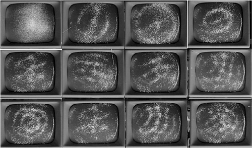
With the setup shown in Fig.5-21, the time-averaging mode has an interferometric sensitivity to target movement, but the dynamic range is limited to s_l(trg).

If we want to increase the dynamic range at the expense of sensitivity, we may simply remove the reference beam in the setup of Fig.5-21. By doing so, we again obtain a signal averaging at an anti-nodal pixel location, but now smearing is due to the loss of correlation, which we incur when the displacement is larger than s_l(trg). The longitudinal size s_l(trg) can be made in the range of, say, 50 to 200μm by an appropriate choice of lens diameter D_L and observation distance z. This mode is called time-averaging without reference, and using it we can observe large-amplitude vibration patterns even in direct sight by eye.

Returning to Fig.5-21, let us comment on the effect of the aperture stop of the objective lens.

The stop affects the speckle size through the diameter D_L because it is a low-pass filter in the frequency (or Fourier) domain of the object. We can use other filtering functions to improve the speckle-image quality. For example, a double-slit stop [12,15] (Fig.5-21) allows increasing the signal amplitude while enhancing the high spatial frequency content of the speckle image picked up by an image photodetector scanned in a raster fashion.

Fig.5-23 ESPI image of a loudspeaker taken with a circular stop and a video high-pass filter (left) and the same with the double-slit stop, high pass, and peak-to-peak rectifier (right).

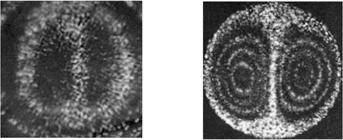
When we combine a structured stop to filter the optical image with an electronic processing of the photodetected signal, the quality of the image is dramatically improved as shown in Fig.5-23. Here, the video output from the photodetector is high-pass filtered and peak-to-peak rectified. This processing yields a more detailed fringe pattern than with the simple high pass and averaging of Fig.5-22.

Now let us consider the pickup of interference images associated with a displacement distribution s(x,y). This is achieved by the frame-subtraction mode of operation of ESPI. As previously noted, the image of a still object is a speckle image that carries no information. Each speckle is an individual interferometer channel, but all channels are uncorrelated because the initial phase φ(x,y) is randomly distributed from pixel to pixel.

Fig.5-24 ESPI image of an aluminum plate before (left) and after (center) the application of a deformation in the center of it. The image at right is the difference of the two and unveils the displacement fringes.

Now, if the target is subjected to a displacement s(x,y), we get another speckle image, again with an intensity distribution uncorrelated from pixel to pixel. However, and this is the important point, the pixel undergoes a brightness variation according to the interferometer phase φ=k (i+r)·s. The variation is singled out by subtracting the initial image from the final image, pixel by pixel.

The result is exemplified in Fig.5-24 for an aluminum plate, observed at rest and after a deformation push at the center. Both initial and final images show no detail, but their difference unveils displacement fringes, each marking a φ(x,y)=2π increment.

The apparatus for the frame-subtraction mode of operation of ESPI is shown in Fig.5-25 [14]. Besides the already described spatial filter in the objective lens stop and the electrical signal processing (high pass and peak-to-peak rectifier), we find a video image recorder. In the recorder, we store the initial image of the object, corresponding to the quiescent state.

The recorded image is read continuously, in synchronism with the photodetector that picks up the image of the object. Then, we may subtract pixel by pixel the initial intensity to the live image intensity. This generates an image containing the fringes associated to the displacement s as, φ=k (i+r)·s.

Fig.5-25 Operation of ESPI in frame subtraction mode. The high-frequency spatial content is enhanced with the appropriate lens stop and by time differentiation of the video signal. The initial speckle image is stored in the recorder so that we can subtract it from the live image presented on the display. As a generalization of the reference beam, an optical correlation block can be used.

The optical correlation block indicated in Fig.5-25 can take several forms. In general, these forms are intended to develop fringes more complicated than the simple displacement measurement [14-20]. For example, instead of measuring the total displacement Z=Z(x,y) of a pixel in the image, we may want to get the relative displacement ΔZ=Z(x,y)- Z(x,y), where Z(x,y) is the average displacement of the target. This mode of operation removes the fringes due to rigid-body translation, a contribution that carries little information usually. We can obtain a speckle map of ΔZ by using, as a reference for superposition to the target image, the scattered light from a ground glass placed in front of the objective lens (Fig.5-26).

Second, in front of the objective lens we may place a beamsplitter with a slight tilt so that two images of the target are formed, laterally shifted by a quantity Δx (Fig.5-26).

Now, let us assume that Δx is less than the transversal (projected) speckle size. Then, we are correlating the fields received by pair of pixels distant of Δx. The result is a measurement of the ΔZ/Δx strain component, in which each fringe indicates an increment ≈λ/2 of the out-of-plane displacement ΔZ relative to points distant of Δx.

Fig.5-26 Optical correlation may take several forms. Left: A partially ground glass provides the reference for the average position of the target. Center: A tilted beamsplitter in front of the objective lens superposes contributions of image pixels shifted of Δx for strain measurement. Right: A mirror pair allows superpose images with different fields of view to get a shearing interferometer.

Another mode of operation of the ESPI is that of shearing measurement. In this interferometer, we want to measure the in-plane strain component S_x=ΔX/Δx following the application of a stress distribution. Here, the displacement X is that of a material point belonging to the target, and x is the laboratory coordinate in which the displacement is viewed. The ratio of their differentials is known as one component of the strain.

One of the several correlation methods developing shear fringes [14,15] is the double mirror [12] shown in Fig.5-26. The target is illuminated from a fixed direction i and viewed from two directions r₁ and r₂. In this way, the phase-sensitive term governing the speckle is , and it only depends on the difference of observation vectors r_1-r₂. As it can be seen in Fig.5-26, the difference vector r₁-r₂ is perpendicular to the lens optical axis or, it is in the plane of the target surface.

From the setup of Fig.5-26, one component of the in-plane strain, let us say S_x=ΔX/Δx, is obtained. Of course, by rotating the setup by 90°, we can also get the other in-plane component of the strain, S_y=ΔY/Δy. We do not report here examples of measurement of strain components, which are rather obvious. The interested reader may consult Refs.[12-19].

Another mode of operation of ESPI instruments is the pulsed mode. In it, we use a pulsed-laser source with adequate coherence to take snapshots of the target. Speckle fringes are formed by frame subtraction of the initial image off the live one. At each instant, we take a snapshot, and a speckle image is acquired. Thus, we can examine objects subjected to periodic stresses, like rotating machinery or turbine blades, and get information on the dynamical deformation undergone along a full cycle of the applied stress. This is valuable information, because it may reveal a pattern of strain evolution forewarning failure.

In processing the ESPI images, we face the problem of phase ambiguity like in any interferometer. Indeed, speckle fringes developed after a displacement s(x,y) obey the equation . As we know, a single trigonometric function of the type cosine leaves an ambiguity in the reconstruction of displacement from the phase φ(x,y).

From the practical point of view, the ambiguity can be removed if we assume that the displacement distribution s(x,y) shall have the least peak-to-peak swing. Then, we may associate a large-width fringe with a local stationary point of s(x,y), that is, a minimum or a maximum. If we also know which point or points in the image are still, we can start from there to draw the paths of steepest variation of s(x,y). In principle, this is the operation, called phase unwrapping by which we are able to reconstruct the s(x,y) distribution [15-20].

Another clean approach to remove ambiguity is to make available a pair of orthogonal signals of the phase shift of the type sine and cosine. This can be easily obtained by applying a phase dither φ_dith to the reference channel [19,21].

To implement the dither, we add a PZT ceramic phase modulator in the reference beam path of Fig.5-21, so that the video signal at the photodetector output becomes cos[φ(x,y)+φ_dith]. If the ceramic is driven by a square wave voltage swinging between 0 and V_π/2, then the phase shift φ_dith swings between 0 and π/2.

By synchronizing the square wave to half the frame frequency of the image pickup, we obtain that, in one frame, the signal is cos k(i+r)·s(x,y) and, in the next frame, is cos [k(i+r)·s(x,y)+π/2]=-sin k(i+r)·s(x,y). Even and odd frames are stored separately and, after averaging, the reconstruction algorithm can be applied to obtain s(x,y).

References

[1] J.W. Goodman, “Statistical Properties of Laser Speckle Patterns”, in Laser Speckle and Related Phenomena, edited by J.C.Dainty, Springer Verlag: Berlin, 2^nd ed., 1981, pp.9-74.

[2] A. Papoulis, “Probability, Random Variables and Stochastic Processes”, 3^rd edition, McGraw Hill: New York, 1991.

[3] D. Middleton, “Introduction to Statistical Communication Theory”, McGraw Hill: New York, 1960; reprinted by IEEE Press: New York, 1996.

[4] J.D. Gaskill, “Linear Systems, Fourier Transforms and Optics”, J.Wiley: New York, 1978.

[5] S. Donati, “Photodetectors”, Prentice Hall: Upper Saddle River, 2000.

[6] S. Donati and G. Martini, “Speckle-Pattern Intensity and Phase Second-Order Conditional Statistics”, Journal of the Opt. Soc. of America, vol. 69 (1979), pp.1690-1694.

[7] M. Norgia, S. Donati, and D. D’Alessandro, “Interferometric Measurements of Displacement on a Diffusing Target by a Speckle Tracking Technique”, IEEE Journal Quant. Electr., vol.QE-37 (2001), pp.800-806. See also “A Displacement-Measuring Instrument Utilizing Self-Mixing Interferometry”, IEEE Trans. Meas. Instrum., vol.IM-52 (2003), pp.1765-1770.

[8] A. Yariv, “Quantum Electronics”, 3rd ed., J.Wiley and Sons: New York, 1989, App. 4.

[9] H. Blinchikoff and A. Zverev, “Filtering in the Time and Frequency Domain”, J.Wiley and Sons: New York, 1976.

[10] S.L. Hahn, “Hilbert Transforms in Signal Processing”, Artech House, Inc.: Norwood, MA, 1996.

[11] M. Sorel, G. Martini, and S. Donati, “Correlation between Intensity and Phase in Speckle Pattern Interferometry”, in Proc. ODIMAP II, 2nd Workshop on Distance Measurement and Applications, edited by S. Donati, Pavia (Italy), 20-23 May 1999, p.132-137.

[12] J.N. Butters, R. James, and C. Wykes, “Electronic Speckle Pattern Interferometry”, in Speckle Metrology, edited by R.K. Erf, Academic Press: New York, 1978, pp.111-158.

[13] R. Jones and C. Wykes, “Holographic and Speckle Interferometry”, 2nd ed., Cambridge University Press: Oxford, 1989.

[14] S. Donati, “A Speckle Pattern Instrument for Real Time Visualization of Vibration and Displacements”, Alta Frequenza, vol.44 (1975), pp.384-386.

[15] O.J. Lokberg and G.A. Slettemoen, “Basic Electronic Speckle Pattern Interferometry”, in Applied Optics and Optical Engineering, vol.X, edited by R.R. Shannon and J.C. Wyant, Academic Press: New York, 1987, pp.455-503.

[16] K.J. Gasvik, “Optical Metrology”, 2nd ed., J.Wiley: Chichester, 1995.

[17] R.S. Sirohi, (editor), “Speckle Metrology”, Marcel Dekker: New York, 1993.

[18] P.K. Rastogi, “Digital Speckle Pattern Interferometry and Related Techniques”, J.Wiley: New York, 2000.

[19] J. Burke, T. Bothe, H. Helmers, C. Kunze, R.S. Sirohi, and V. Wilkens, “Spatial Phase Shifting in ESPI: Influence of Second-Oorder Speckle Statistics on Fringe Quality”, in Fringe ′97, Automatic Processing of Fringe Patterns, edited by W.J. Jüptner and W. Osten, Wiley Europe: London, 1997, pp. 111-119.

[20] D. Paoletti and G. Schirripa Spagnolo, “Interferometric Methods for Artwork Diagnostics”, Progress in Optics, vol.35 (1996), pp.197-255.

[21] G. Martini, M. Facchini, and D. Parisi, “Automatic Phase-Stepping in Fiber-Optic ESPI by Closed-Loop Gain Switching”, IEEE Trans. Meas. Instr., vol.IM-49 (2000), pp.823-828.