
Chapter 19. Introduction to Adsorption, Chromatography, and Ion Exchange
In the first 14 chapters, we looked at separation techniques such as distillation and extraction that are often operated as steady-state, equilibrium-staged separations. Exceptions were batch distillation in Chapter 9 and batch extraction in Section 13.6. In Chapter 17 we studied both batch and continuous crystallization. Outlet concentrations can be found from equilibrium calculations, but crystal size distributions required population balances. In Chapter 18 we studied membrane separations that are not operated as equilibrium processes; however, well-mixed membrane separators are analogous to flash distillation, and staged models are useful for integrating mass balances and rate expressions for more complex flow patterns. Since membrane processes are normally operated at steady state, analysis is usually straightforward. In this chapter we study three closely related processes that are rarely operated or analyzed as steady-state, equilibrium-staged systems. These sorption processes are usually operated in packed columns in a cycle that includes feed and regeneration steps; thus, as normally operated, these processes are inherently unsteady state.
Adsorption (note the “d,” not a “b”) involves contacting a fluid (liquid or gas) with a solid (the adsorbent). One or more of the components of the fluid are attracted to the adsorbent surface. These components can be separated from components that are less attracted to the surface. Adsorption is commonly used to clean fluids by removing components from fluid or to recover the components. Many homes and apartments use a carbon “filter” (actually, an adsorber) for water purification. Chromatography is a similar process that uses a solid packing material (an adsorbent or other solid that preferentially attracts some components in a mixture), but operation is devised to separate components from each other. You may have analyzed composition of samples with analytical chromatography (gas or liquid) in labs. In ion exchange the solid contains charged groups that interact with charged ions in the liquid. Best-known application of ion exchange is water softening to remove calcium and magnesium ions and replace them with sodium ions. These separation methods are complementary to equilibrium-staged processes. They are often used for chemical analysis, separation of dilute mixtures, and separation of difficult mixtures where equilibrium-staged separations either do not work or are too expensive.
The three separation techniques studied in this chapter are similar, since a solid phase causes separation. When we want to lump them together, we will call them sorption processes. The general term for an adsorbent, ion exchange resin or chromatographic packing is sorbent (it sounds like it would be good to eat, but it is not). The most common equipment for sorption processes is a stationary packed bed of solid. The solid in sorption systems directly causes separation, which is different than packed beds for equilibrium separations where solid is inert but increases interfacial area and mass transfer coefficients between gas and liquid. If feed is introduced continuously into a sorption packed bed, the bed will eventually saturate (e.g., approach feed concentration) and separation will cease. Much of the art and expense of designing these systems is in the regeneration step that removes component from solid. Regeneration is so important that different processes are often named on the basis of the regeneration method used.
This chapter is a simplified introduction to the fascinating and valuable sorption separation methods. Three-fourths of the chapter rely on equilibrium analysis—mass transfer is introduced in Section 19.6. Development is similar, but at a more introductory level, to that in Wankat (1986; 1990). Once you understand this chapter, you will be able to discuss these techniques with experts and will be prepared to begin more detailed explorations of these methods in more advanced books (e.g., Do, 1998; Ruthven, 1984; Ruthven et al., 1994; Yang, 1987; 2003).
Note: A nomenclature list for this chapter is included in the front matter of this book.
19.0 Summary—Objectives
In this chapter basic concepts for adsorption, chromatography, and ion exchange separations are developed. At end of this chapter, you should be able to satisfy following objectives:
1. Determine equilibrium constants from data and use equilibrium equations in calculations
2. Explain in your own language how different sorption processes (e.g., elution chromatography, temperature swing adsorption [TSA], pressure swing adsorption [PSA], simulated moving beds [SMB], monovalent-monovalent ion exchange, and water softening) work
3. Explain the meaning of each term in development of solute movement equations and use this theory for both linear and nonlinear isotherms to predict outlet concentration and temperature profiles for a variety of different operations, including elution chromatography, TSA, PSA, SMB, and ion exchange
4. Explain the meaning of each term in column mass and energy balances and in mass and heat transfer equations
5. Use Lapidus and Amundson solution plus superposition to determine outlet concentration profiles for linear adsorption and chromatography problems
6. Use theory of linear chromatography with very small pulses to analyze chromatography systems
7. Use length of unused bed (LUB) theory in combination with experimental data to design columns
8. Use Aspen Chromatography to simulate adsorption and chromatography systems.
19.1 Sorbents and Sorption Equilibrium
Since sorption and sorbents are quite different from equilibrium-staged processes and membrane separations studied earlier, we need to first carefully define terms needed to study and design these systems. After a short description of different sorbents, equilibrium behavior of sorbent systems is introduced. Then the last fundamental piece required is mass transfer characteristics of sorbents and sorption processes.
19.1.1 Definitions
The most common contacting device for adsorption, chromatography, and ion exchange is a vertical packed bed, shown schematically in Figure 19-1. Particles are packed in the cylindrical column of cross-sectional area Ac and length of packed section L. Some type of support netting or frit is used at the bottom of the packed section, and a hold-down device such as a net or frit is used at the top of the packed section. Figure 19-1 illustrates a number of important variables. External porosity εe is the fraction of column volume that is outside the particles. To some extent value of εe depends on particle shape (e.g., εe is smaller for spheres than for irregular shaped particles) and packing procedure used. It is important to have a uniformly packed column with a constant value of εe. Internal porosity εp is the fraction of volume of pellets that consists of pores and thus is available to fluid. Total volume available to fluid is
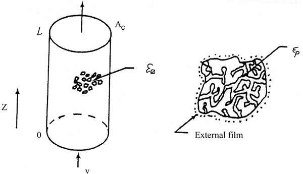
FIGURE 19-1. Schematic of adsorption column and particle (Wankat, 1986), reprinted with permission, copyright 1986, Phillip C. Wankat
From this equation we can define total porosity εT as sum of all the voids:
Porosities are dimensionless.
Although fluid can fit into all pores, molecules such as proteins may be too big to fit into some or all pores. This size exclusion can be quantified in terms of a dimensionless parameter Kd where Kd,i = 1.0 if molecule i can penetrate all pores and Kd,i = 0 if molecule i can penetrate none of the pores. The value of Kd,i for a given molecule i can be between 0 and 1, since pores are not of uniform size. Volume available to molecule i is
This picture is useful but does not match all adsorbents. Gel-type ion-exchange resins have no permanent pores. Instead they consist of a tangled network of interconnected polymer chains into which solvent dissolves. In effect, εp = 0. Macroporous ion exchange resins have permanent pores and εp > 0, but often Kd,i < 1.0 for large molecules. Many activated carbons have both macropores and micropores; thus, there are two internal porosities. Molecular sieve zeolite adsorbents are used as pellets that are agglomerates of zeolite crystals and a binder such as clay. In this case, there is an interpellet porosity (typically, εe ∼ 0.32), an intercrystal porosity (εp1 ∼ 0.23), and an intracrystal porosity (εp2 ∼ 0.19), which has Kd,i ≤ 1.0 (Lee, 1972).
Two different velocities are typically defined for the column shown in Figure 19-1. Superficial velocity, which is easy to measure, is average velocity volumetric flow of fluid would have in an empty column. Thus
where Q is volumetric flow rate (e.g., in m3/s), cross-sectional area ![]() and vsuper is in m/s. Interstitial velocity vinter (m/s) is average velocity fluid has flowing between particles. Since the cross-sectional area actually available to fluid is εe Ac, a mass balance on flowing fluid is
and vsuper is in m/s. Interstitial velocity vinter (m/s) is average velocity fluid has flowing between particles. Since the cross-sectional area actually available to fluid is εe Ac, a mass balance on flowing fluid is
vinter εe Ac = vsuper Ac
which gives
Since εe is less than 1.0, vinter > vsuper. Very large molecules that are totally excluded from pores and are not adsorbed move at an average velocity of vinter.
There are also different densities of interest. Fluid density ρf (e.g., in kg/m3) is familiar. A second density is structural density ρS (kg/m3) of solid. This is solid density if it is crushed and compressed so that there are no pores and all air is removed. Particle or pellet density ρp is average density of particles consisting of solid plus fluid in pores.
Manufacturers often report a bulk density ρb of adsorbent. This density is weight of adsorbent as delivered, which includes fluid in pores and between particles, divided by container volume. Bulk density can be calculated from the other densities:
Bulk and particle densities are also in kg/m3. If fluid is a gas with ρf << ρp,
Unfortunately, it is often unclear which density is being referred to. By comparing values given by the manufacturer to approximate values listed in Table 19-1, one may be able to determine which density is being referred to.
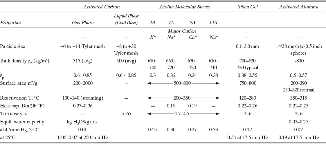
TABLE 19-1. Properties of common adsorbents (Humphrey and Keller, 1997; Reynolds et al., 2002; Ruthven et al., 1994; Wankat, 1990; Yang, 1987)
One last useful definition is tortuosity τ. Tortuosity relates effective diffusivity in pores Deffective to molecular diffusivity in free solution, Dmolecular:
Note that τ is dimensionless. Equation (19-4) was originally derived from geometric considerations using a simple geometric model. However, measured values of τ are often much larger than expected from purely geometric arguments because diffusion is hindered by walls or at pore mouth. Thus we will treat τ and Deffective as empirical (experimentally measured) quantities. Molecular diffusivity can be determined experimentally, but there are also a number of well-known methods to predict Dmolecular (see Section 15.3).
19.1.2 Sorbent Types
A variety of sorbents are used commercially for separations. We first present a very short introduction to common commercially used adsorbents. If more detail is required, refer to Yang’s (2003) very detailed analyses. Commercially important adsorbents are highly porous and have high surface areas per gram. This high surface area greatly increases capacity for adsorption. Typically, 98% of adsorption occurs in pores inside particles and only 2% on external surface. Molecules that adsorb are called adsorbate. Adsorbed molecules typically have a density close to that of a liquid. Thus, there are major density and volume changes when gases are adsorbed but very small changes when liquids are adsorbed.
Activated carbon is a very porous adsorbent with a carbon backbone but a number of other species such as oxides of carbon on the surface. Since activated carbon is inexpensive, strongly adsorbs organic compounds, and has a large number of applications, it is the most commonly used adsorbent (Bonsal et al., 1988; Faust and Aly, 1987). It is produced by carbonizing a material such as wood, coke, or coconut shells. Activation is typically done with carbon dioxide or steam to create porous structure and to oxidize the surface. Additional chemical treatments such as with iodine can be used to produce specialty carbons (Yin et al., 2007). Carbons are produced for both liquid and gas separations. Because starting materials and chemical treatments vary, different activated carbons can have very different properties. Thus, average values reported in Table 19-1 should be used only for very preliminary calculations and approximate designs. Experimental data on a particular brand, grade, and size of activated carbon should be used for more detailed designs.
Because activated carbon has essentially a nonpolar surface, water is adsorbed weakly, often by capillary condensation in gas systems (Yang, 1987). Thus, many organic compounds are much more strongly adsorbed than water. This makes activated carbon the usual adsorbent of choice for processing aqueous solutions and humid gases. Since activated carbon is commonly used to remove organic compounds from water, equilibrium isotherms have been measured for a large number of compounds (Dobbs and Cohen, 1980). Activated carbon is also frequently used to adsorb small amounts of organics from gases, process sugar, purify alcohol, provide personal protection as part of the complex mixture of adsorbents included in gas masks, and many other applications.
Carbon molecular sieves (CMS) have very tightly controlled pore structures. They are prepared in a manner that is similar to activated carbon except there is often an additional step in which a hydrocarbon is cracked or polymerized on the surface to create desired uniform pore size (Ruthven et al., 1994). Because of extra care required in processing and because of patent protection, CMS are significantly more expensive than activated carbon. Currently, CMS are commonly used for producing pure nitrogen from air. Unlike the vast majority of commercial adsorbents, CMS can separate based on different diffusion rates instead of different equilibrium behavior. Design of kinetic adsorption processes is highly specialized (e.g., see Ruthven et al., 1994).
Zeolite molecular sieves are crystalline aluminosilicates with general formula
Mx/n[(AlO2)x (SiO2)y]z H2O
where M represents a metal cation such as lithium, sodium, potassium, or calcium of valence n; x and y are integers (y ≥ x); and z is number of water molecules per unit cell. Since zeolites are crystals, pores have exact dimensions (Ruthven, 1984; Ruthven et al., 1994; Yang, 1987, 2003). Thus, zeolites can be used to separate based partially on steric exclusion, although separations where steric exclusion is not employed are more common. A large number of synthetic and naturally occurring zeolites are known, although not all are used commercially as adsorbents. Commercial applications of zeolites as adsorbents include drying air and natural gas, drying organic liquids, removal of carbon dioxide, separation of ethanol and water to break the azeotrope, and separation of oxygen from nitrogen in air. The major steric exclusion application is separation of straight-chain hydrocarbons (used for biodegradable detergents) from branched-chain hydrocarbons. Zeolite properties are reported in Table 19-1.
Silica gel is an amorphous solid made up of colloidal silica SiO2 that is normally used in a dry granular form. (The name “gel” arises from the jellylike form of material during one stage of its production [Reynolds et al., 2002].) Silica gel is commonly used for drying gases and liquids because it has a high affinity for water. Silica gel is complementary to zeolites, since it is cheaper and has a higher capacity at water vapor pressures greater than about 10 mm Hg (Humphrey and Keller, 1997) but cannot dry to as low water content. Columns with a layer of silica gel at feed end and a layer of zeolite at product end are commonly used for drying, since they combine best properties of both adsorbents. Note that silica gel can be damaged by liquid water. Silica gel properties are reported in Table 19-1.
Activated alumina Al2O3 is also commonly used for drying gases and liquids and is not damaged by immersion in liquid water. It is produced by dehydrating aluminum trihydrate Al(OH)3 by heating. Activated alumina has properties that are similar to silica gel, although it is physically more robust. It competes with silica gel in drying applications, although its capacity is a bit lower at water vapor pressures greater than about 1 mm Hg (Humphrey and Keller, 1997). Activated alumina is also used in water treatment to selectively remove excess fluoride. Activated alumina properties are listed in Table 19-1.
A large number of other materials are used commercially as adsorbents. These include an uncharged form of organic polymer resins commonly used for ion exchange (see Section 19.5). Although considerably more expensive, these resins compete with activated carbon for recovery of organics. Activated bauxite is an impure form of activated alumina. A number of clays are used for purification of vegetable oils. Bone char, which has both adsorptive and ion exchange capacities, is used in purification of sugar.
When common adsorbents are used in chromatography applications (Cazes, 2005), they are used as much smaller particles with a much tighter particle size distribution. A number of specialized packing materials have been developed for chromatographic applications. In gas-liquid chromatography a high-boiling, nonvolatile liquid (the stationary phase) is coated onto an inert solid such as diatomaceous earth. A similar method called liquid-liquid chromatography coats an immiscible liquid on an inert solid. This packing is now often replaced with bonded packing where stationary phase, often a C8 or a C18 compound, is chemically bonded to inert solid, which is usually silica gel. Equilibrium behavior of these specialized packings is usually similar to gas-liquid absorption or liquid-liquid extraction, but because of presence of inert solid, equipment and operating principles are similar to adsorption-chromatography.
19.1.3 Adsorption Equilibrium Behavior
Equilibrium behavior of adsorbents is usually determined as constant temperature isotherms. Valenzuela and Myers (1989) present the most extensive compilations of isotherm data, which is a good entry point into the large literature on adsorption equilibrium measurements and theories. Basmadjian (1984) has extensive data on water isotherms from gases and liquids. Dobbs and Cohen (1980) and Faust and Aly (1987) present adsorption data for common pollutants.
Typical isotherm data for gas adsorption of single components are shown in Figures 19-2A and 19-2B. Figure 19-2A shows adsorption of different gasses. Hydrogen is least strongly adsorbed, followed by methane. Adsorption is strongest for ethane and ethylene, and then maximum adsorption is less for propane, although its adsorption is stronger at low partial pressures. Each adsorbent has an optimum size molecule for maximum adsorption. Figure 19-2B compares adsorption of ethylene on different adsorbents.
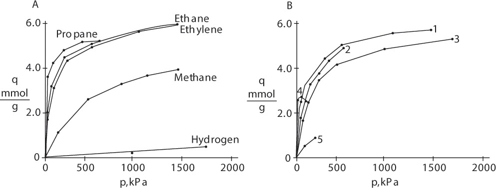
FIGURE 19-2. Adsorption isotherms for pure gases: (A) Gases on Columbia grade L activated carbon at 310.92 K (Ray and Box, 1950; Valenzuela and Myers, 1989), (B) Ethylene on different adsorbents at varying temperatures (Valenzuela and Myers, 1989). Key: 1 = Columbia grade L activated carbon at 310.92 K. 2 = Taiyo Kaken Co., Japan, attrition resistant activated carbon at 310.95 K. 3 = Pittsburgh Chemical Co. BPL activated carbon at 301.4 K. 4. Union Carbide 13X Linde zeolite at 298.15 K. 5 = Davison Chemical Co. silica gel at 298.15 K.
At low concentrations or partial pressures, isotherms are often linear. As gas partial pressure increases, isotherms become nonlinear—they curve. Equilibrium data for adsorption of single gases are often fit with the Langmuir isotherm,
where qA is amount of species A adsorbed and qA,max is maximum amount of species A that can adsorb (kg/kg adsorbent or mol/kg adsorbent), pA is partial pressure of species A (mm Hg, kPa, or other pressure units), and KA is adsorption equilibrium constant in suitable units. Note that for very small partial pressures, KA,p pA << 1.0 and Eq. (19-5a) simplifies to a linear form:
while at very high partial pressures, KA,p pA >> 1.0, Eq. (19-5a) simplifies to
This is a horizontal line that represents saturation of adsorbent.
For liquids isotherms are usually written in terms of liquid concentration cA (mol/m3 or kg/m3). For example, the Langmuir isotherm for a liquid is
In the linear limit when KA cA << 1.0, this simplifies to
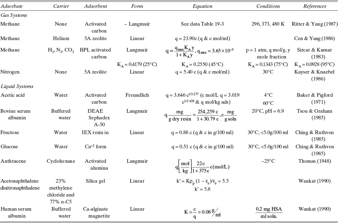
Adsorption equilibrium constants KA,c and K′A,c are in different units for liquid systems than for gas systems. Equilibrium constants for several systems are listed in Table 19-2.
Isotherm data at different temperatures invariably shows that there is less material adsorbed as temperature increases. Adsorption equilibrium constants often follow an Arrhenius form:
where KAo is a pre-exponential factor, ΔH is heat of adsorption (e.g., in J/kg), R is gas constant, and T is absolute temperature (e.g., in K). Since adsorption is invariably exothermic, ΔH is negative. If Arrhenius form is followed, a plot of ln KA vs. 1/T will be a straight line with a slope of –ΔH/R. Don’t automatically assume that data follow an Arrhenius form. Plot the data and check whether points are on a straight line. Typically, qA,max slowly decreases as temperature increases.
Langmuir used a simple kinetic argument (e.g., Wankat, 1990) to derive Eqs. (19-5a) and (19-6a). When this argument is used, qA,max is coverage obtained with a monolayer. Langmuir’s isotherm can also be derived with a statistical mechanics argument (e.g., Ruthven, 1984). Data are often correlated with a Langmuir isotherm even when there is reason to believe that the mechanism postulated by Langmuir is incorrect. For liquid systems it is common to write the Langmuir isotherm as
and there is no implication that a or b have physical interpretations. Correlation of data is best done by multivariable regression techniques but is often done by plotting c/q vs. c (or p/q vs. p). In these plots Langmuir isotherm data plot as a straight line (see Example 19-1 and homework Problem 19.D1).
The Langmuir isotherm is thermodynamically correct for single-component systems. It has been used to develop a variety of other isotherms, such as BET isotherm (multiple adsorbate layers), Langmuir-Freundlich isotherm, and linear-Langmuir isotherm (add a linear isotherm and Langmuir isotherm). Langmuir isotherms are also commonly extended to adsorption of multicomponent mixtures. For example, for simultaneous adsorption of components A and B, Eq. (19-6c) becomes
This equation correctly predicts that two adsorbates compete for adsorption sites. That is, if concentration of B increases, amount of A adsorbed decreases. Unfortunately, very few systems follow Eqs. (19-8) exactly, and if aA does not equal aB, Eq. (19-8) is not thermodynamically consistent (LeVan and Vermeulen, 1981). Despite these problems Eq. (19-8) and its extensions to more components are commonly used for theories for multicomponent adsorption because this is the simplest form that shows competition.
A thermodynamically correct approach, ideal adsorbed solution (IAS) theory, uses Langmuir isotherms for single-component isotherms. Details of IAS and additional isotherms are discussed by Do (1998), Ruthven (1984), Valenzuela and Myers (1989), and Yang (1987; 2003).
EXAMPLE 19-1. Adsorption equilibrium
Experimental equilibrium data for adsorption of methane on Calgon Carbon Corp. PCB activated carbon are listed in Table 19-3. Determine if Langmuir isotherm, Eq. (19-5a), is a good fit for data at T = 373 K and if adsorption equilibrium constant KA,p follows Arrhenius form, Eq. (19-7a). Other values for KA,p are KA,p (296 K) = 2.045 × 10⁻³ (kPa)–1 and KA,p (480 K) = 1.888 × 10⁻⁴ (kPa)–1 (see Problem 19.D1).
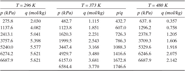
TABLE 19-3. Equilibrium data for methane on Calgon PCB activated carbon (Ritter and Yang, 1987; Valenzuela and Myers, 1989)
Solution
A. Define. Find best-fit parameter values for KA,p and qA,max in Eq. (19-5a) for 373 K data. Then plot isotherm data and Langmuir isotherm to determine if this is a good fit. Finally, determine if KA,p data satisfies Eq. (19-7a) and find ΔH.
B, C. Explore and plan. Equation (19-5a) can be rearranged so that it will be a straight line. Multiply both sides by (1 + KA,ppA) and divide by qA,
If Langmuir isotherm is valid, a plot of pA/qA vs. pA will be linear. Direct nonlinear fitting of the raw data can also be done instead of linearization.
Take n.atural log of both sides of Arrhenius relationship, Eq. (19-7a):

A plot of ln KA,p vs. (1/T) will be a straight line if Arrhenius equation is followed. We can also check to see if qmax follows an Arrhenius form.
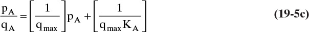
D. Do it. Values of p/q at 373 K are listed in Table 19-3. A plot of p/q vs. p is shown in Figure 19-3A. Intercept = 360 = 1/qmaxKAp.
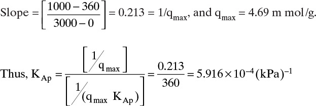
FIGURE 19-3. Plots of equilibrium data for Example 19-1; (A) plot to give straight line for Langmuir isotherm, (B) Langmuir isotherm, (C) check on Arrhenius relationship (T in K)
and Langmuir isotherm at 373 K is
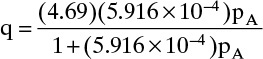
A plot of this isotherm is shown in Figure 19-3B. Agreement between Langmuir curve and data are quite good. Values for Arrhenius plot are,
Plots of ln KA,p vs. 1/T and ln qmax vs. 1/T are both shown in Figure 19-3C. Clearly data for both plots are well fit by straight lines and Arrhenius relation is satisfied for both KA,p and qmax. From Eq. (19-7b) for the ln KA,p plot, slope = –ΔH/R:

E. Check. Figure 19-3B is a check on fit of Langmuir constants. Since agreement between curve and data points is quite good, the analysis is confirmed. Close agreement on the Arrhenius plot is another check on analysis procedure.
F. Generalize. Fit to a straight line in Figure 19-3C is closer than for many other adsorption systems. Remember that although amount adsorbed generally decreases as temperature increases, adsorption does not always follow an Arrhenius relationship. Note that values of qmax often do not follow an Arrhenius relationship, although this system does.
19.2 Solute Movement Analysis for Linear Systems: Basics and Applications to Chromatography
Packed columns similar to Figure 19-1 are the most common contacting devices used for adsorption and chromatography. Although there are exceptions, they are usually operated vertically with flow parallel to the column axis. Adsorption, chromatography, and ion exchange in packed columns are inherently unsteady-state or batch type processes. Since sorbent is stationary, it saturates at the feed concentration if feed enters the column continuously. Thus, there must also be a regeneration step that removes most of the sorbate from packing. Common regeneration methods are to use an inert purge stream, change temperature, change pressure, and use a desorbent. After regeneration, there may be an optional cooling, drying, repressurization, or washing step. The next cycle starts with a feed step. These processes are analyzed in Sections 19.2 to 19.8 using increasingly complex analysis procedures. In this section we start with the simplest theory, solute movement theory for linear isotherms, applied to elution chromatography, the simplest process to analyze.
Complete analysis of sorption processes requires computer simulation with a rather complex simulation program to solve coupled algebraic and partial differential equations. Unfortunately, simulators often do not provide a physical picture of why separation occurs, and once a result is obtained simulators don’t tell what to do to improve the separation. A relatively simple tool that is based on physical arguments and can be solved with pencil and paper (or a spreadsheet) will prove to be very useful even if it is not completely accurate. Solute movement analysis is a tool that allows engineers to use physical reasoning to understand results from experiments or simulations. The role of solute movement analysis in sorption processes is analogous to the role of McCabe-Thiele diagrams in distillation, absorption, and extraction. Solute movement theory is used to understand separations and for troubleshooting, not for final design.
19.2.1 Movement of Solute in a Column
Solute or sorbate within the packed section of a column can be in one of three locations. The solute can be in interstitial void space εe and be moving at interstitial velocity vinter. If solute is in intraparticle voids [(1 – εe) εp] or sorbed to stationary solid, it will have a net axial velocity of zero. In other words, solute molecules are either scooting forward axially at a high velocity (remember that vinter is greater than vsuper), or they aren’t moving at all. Average solute velocity us is
This fraction can be calculated by considering distribution of an incremental change in solute concentration Δc (e.g., in mol/m3) and its corresponding change in the amount sorbed Δq (e.g., in mol/kg adsorbent). Amount in each location can be determined by doing an inventory of moles.

where Kd is the fraction of pores that molecules can squeeze into. This term becomes important in size exclusion chromatography, which separates molecules based on size and ideally has no adsorption, Δq = 0 (Wu, 2004).
Both Eqs. (19-11a) and (19-11b) are in moles adsorbate if c is mol/m3.

The Kd term is not included in Eq. (19-11c), since we assume Δq is based on a measurement that automatically includes any steric hindrance. Equation (19-11c) will also be in moles adsorbate. If q and c are in different units than in this derivation, the mass balances will be slightly different [compare Eqs. (19-14a) through (19-14c) to Eq. (19-13)].
Inserting Eq. (19-11) into Eq. (19-10), we obtain
After Eq. (19-12) is substituted into Eq. (19-9), the result can be simplified to
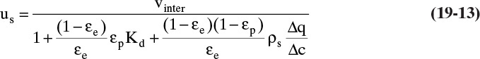
The exact form of Eq. (19-13) depends on units of equilibrium data. For example, if isotherm expression is q = f(x) with q in kg solute/kg solid and x in mass fraction (kg solute/kg fluid), then there must be a ρF (kg fluid/m3) term in Eqs. (19-11a) and (19-11b), and Δx replaces Δc in these equations. Then Eq. (19-13) becomes
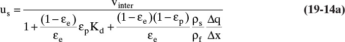
If q and c are both in mol/m3, equation for us is obtained by eliminating ρs from Eq. (19-13).
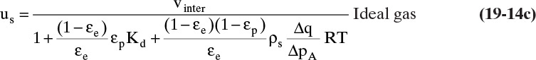
For gas systems equilibrium is often expressed in terms of partial pressure, pA [e.g., Eqs., (19-5a) and (19-5b)]. Solute velocity for gases is then
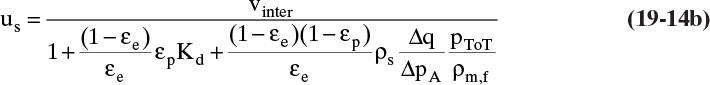
where ρm,f is fluid molar density. For an ideal gas, ρm,f = ptot/RT and ptot/ρm,f = RT. Thus, for ideal gases,
In some ion exchange and biochemical systems c and q are both in g/L or mol/L. Then Δq is also in g/L or mol/L, and the ρs term in Eqs. (19-11c), (19-12), and (19-13) does not appear. The result is
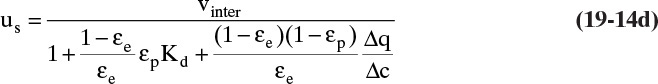
Equations (19-13) and (19-14) allow us to calculate average velocity of solute if we can calculate (Δq/Δc), (Δq/Δx), or (Δq/ΔpA). Since detailed derivations of Eqs. (19-14a) to (19-14d) were not presented, I strongly encourage you to do at least one part of Problem 19.C2. Understanding derivations will be helpful in Sections 19.2.2 to 19.5 when we insert appropriate isotherms into Eqs. (19-13) and (19-14). In the vast majority of commercial sorption separations, solute velocity depends only on equilibrium behavior (Δq/Δc), (Δq/Δx), or (Δq/ΔpA) and packed column properties, not on mass transfer rates. Mass transfer is critically important to determine how solute spreads from the average (see Sections 19.6 to 19.8).
19.2.2 Solute Movement Theory for Linear Isotherms
The theory becomes simplest when a linear isotherm, Eq. (19-5b) or (19-6b), is used. Since almost all equilibrium data becomes linear at low enough concentrations or partial pressures, there are a number of real applications of linear isotherms.
When Eq. (19-6b) is valid, ![]() and Eq. (19-13) becomes
and Eq. (19-13) becomes
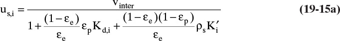
for any adsorbate i. Terms do not depend on concentration of adsorbate i. Thus, at low concentrations where linear isotherms are valid, solute velocity is constant. Solute velocity us,i depends on temperature, since ![]() depends on temperature [e.g., following Eq. (19-7a)]. If we have a number of different solutes with different values of equilibrium constant, the weakest sorbed solute (lowest value of
depends on temperature [e.g., following Eq. (19-7a)]. If we have a number of different solutes with different values of equilibrium constant, the weakest sorbed solute (lowest value of ![]() ) moves fastest, and the strongest sorbed solute (highest value of
) moves fastest, and the strongest sorbed solute (highest value of ![]() ) moves slowest. Since they move at different speeds, they can be separated. A single-porosity form of this equation is also commonly used [see Problem 19.C5, which includes Eq. (19-15b)].
) moves slowest. Since they move at different speeds, they can be separated. A single-porosity form of this equation is also commonly used [see Problem 19.C5, which includes Eq. (19-15b)].
To visualize what this looks like, we start with an initially clean (cA = 0) packed column. At time t0, we start adding a feed with concentration cA,F at a known interstitial velocity. Equation (19-15a) can be used to calculate solute velocity us,A (the numerical calculation procedure is illustrated in Example 19-2). In Figure 19-4A the solute movement or characteristic diagram for this process is plotted. Solute starts at z = 0 at time t0 and moves upward at velocity us,A, which is slope of the characteristic line shown in the figure. The procedure will probably be easiest to understand after you study Example 19-2. Concentrations in the column are shown at four times in Figures 19-4B through 19-4E. Solute moves upward in a wave at a constant velocity us,A. If adsorption is strong, the wave moves slowly, whereas if adsorption is weak, it moves quickly. Waves for nonlinear systems are shown later in Figure 19-15.
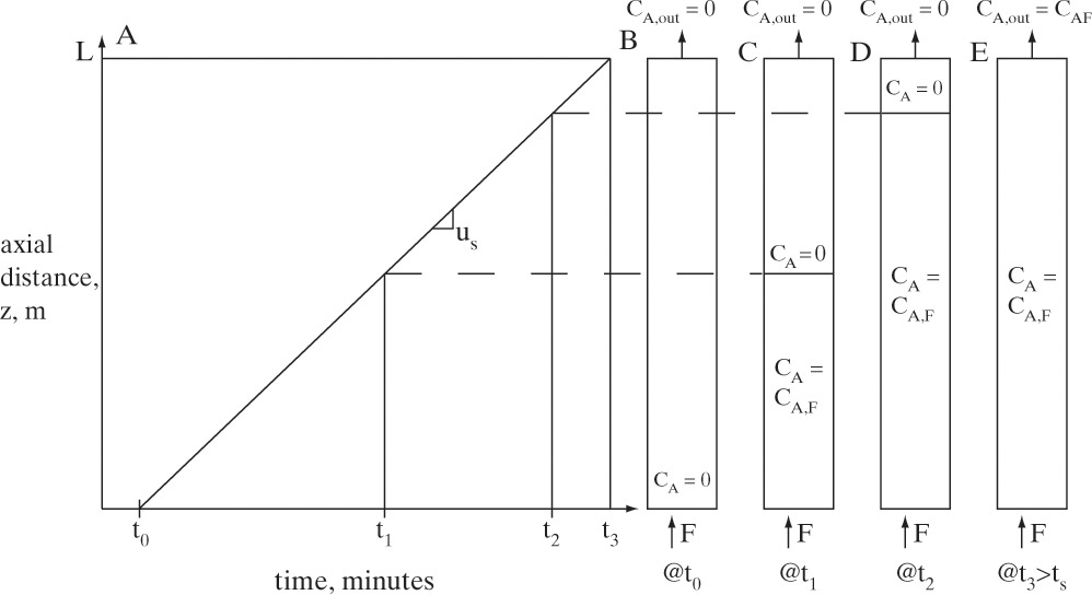
FIGURE 19-4. Wave movement for step change in feed concentration. (A) Solute movement diagram for linear isotherm. B, C, D, E are concentrations in column at t = t0, t1, t2, and t3, respectively. Since t3 = breakthrough time tbr = L/us,A, entire column and outlet are at CA,F
For systems with weight fraction units, ![]() or
or ![]() where q is in kg solute/kg adsorbent and x or y is in kg solute/kg fluid (weight fraction), Eq. (19-14a) becomes
where q is in kg solute/kg adsorbent and x or y is in kg solute/kg fluid (weight fraction), Eq. (19-14a) becomes
For ideal gases with ![]() Eq. (19-14c) becomes
Eq. (19-14c) becomes

With linear isotherms the denominator in Eqs. (19-15a) through (19-15d) is independent of concentration. Thus, for purposes of algebraic manipulation, it is convenient to write these equations as
Although very convenient, linear isotherms find limited applications in industrial processes. To decrease column diameters and thus reduce costs, most industrial separations are done at high concentrations or very close to solubility limits. Since isotherms are probably nonlinear and use of linear isotherms will lead to large errors, one needs to use nonlinear theories (Section 19.6) for concentrated systems. However, linear isotherms are appropriate for many chromatography applications, since solute concentrations are often very low.
19.2.3 Application of Linear Solute Movement Theory to Purge Cycles and Elution Chromatography
The simplest regeneration method is a purge using an inert carrier gas for gas systems or an inert solvent for liquid systems. This cycle can be operated co-flow (Figure 19-5A) or counterflow (Figure 19-5B). When purge gas or liquid enters the column, partial pressure or concentration of adsorbate drops, since it is being diluted. This drop in concentration causes adsorbate to desorb (see Figure 19-2), thus, allowing it to be flushed from the column. The ideal carrier gas or solvent has the following properties: easy to separate from adsorbate, easy to remove from bed, nontoxic, nonflammable, available, and inexpensive. For purge gas systems, nitrogen and hydrogen are close to ideal as carrier gases. Since adsorbate is diluted, purge cycles are not commonly used for large-scale commercial adsorption processes.
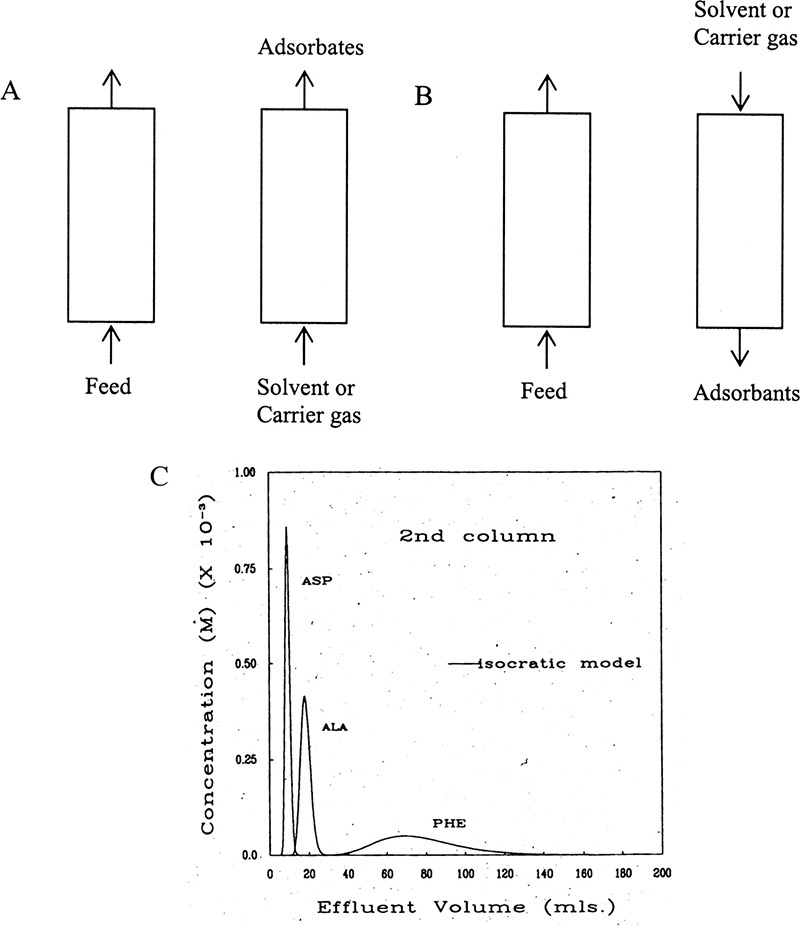
FIGURE 19-5. Purge systems. (A) co-flow (e.g., elution chromatography), (B) counterflow, (C) outlet concentrations for elution chromatography of aspartic acid (asp), alanine (ala), and phenylalanine (phe) on cation exchange resin (Agosto et al., 1989). Reprinted with permission from Ind. Eng. Chem. Research, 28, 1358 (1989), copyright 1989 American Chemical Society.
Purge cycles are commonly used in elution chromatography, particularly in analytical chemistry. Elution chromatography involves input of a feed pulse into a packed column followed by co-flow (Figure 19-5A) of an inert solvent or carrier gas. (If solvent or carrier gas also adsorbs, the process can become gradient or displacement chromatography, which are discussed later.) Columns can be packed with adsorbents or chromatography packings mentioned previously. If solutes have different equilibrium isotherms, solutes will move at different velocities and will be separated (Figure 19-5C). Both gas and liquid chromatography are commonly operated in elution mode to determine compositions of unknown samples. Large-scale elution chromatography systems are also becoming more common, particularly in pharmaceutical and fine chemical industries. Detailed design considerations for large-scale biochromatography systems are discussed in detail by Ladisch (2001). Dilution that is inherent in purge operations makes these processes expensive for large-scale separation, but with complicated feeds there may be no better alternative.
EXAMPLE 19-2. Linear solute movement analysis of elution chromatography
A 1-meter column is packed with activated alumina. The column initially contains pure liquid cyclohexane solvent. At time t = 0, a feed pulse that contains 0.0001 mol/L anthracene and 0.0002 mol/L naphthalene in cyclohexane is input for 10.0 minutes. Superficial velocity is 20 cm/min for both feed and purge steps. Use solute movement theory to predict outlet concentrations.
Data: Bulk density (fluid is air) = 642.6 kg/m3, εp = 0.51, εe = 0.39, ρf (cyclohexane) = 0.78 kg/L. ![]() adsorbent and
adsorbent and ![]() adsorbent where A = anthracene and N = naphthalene. Kd = 1.0 for both anthracene and naphthalene.
adsorbent where A = anthracene and N = naphthalene. Kd = 1.0 for both anthracene and naphthalene.
A. Define. Apparatus is sketched in Figure 19-5a. We want to find when anthracene and naphthalene pulses exit.
B. Explore. Equation (19-15) can be used to determine numerical values of us,A and us,N. Lines drawn on a solute movement diagram with these slopes from start (t = 0 min) and end (t = 10 min) of feed pulse outline movement of average molecules of anthracene and naphthalene. Since ![]() , us,N > us,A, and naphthalene should exit first.
, us,N > us,A, and naphthalene should exit first.
C. Plan. Calculate us,N and us,A. Plot solute movement diagram for a 10-minute feed pulse.
D. Do it. Interstitial velocity can be determined from Eq. (19-2b):
vinter = vsuper /εe = (0.2 m/min)/0.39 = 0.513 m/min.
Structural density can be determined by rearranging Eq. (19-3c):
ρs = ρb /[(1 – εe)(1 – εp)] = (642.6 kg/m3)/(0.61)(0.49) = 2150 kg/m3
Solute velocities can now be calculated from Eq. (19-15):
Note that we converted ![]() from L/kg to m3/kg. Similarly, us,N = 0.0182 m/min. These solute velocities are slopes for each solute on the solute movement diagram (Figure 19-6A). Lines for each solute can be drawn from start and finish of the feed pulse. Resulting solute pulses or waves exit at z = L = 1.00 m, as shown in Figure 19-6B. Naphthalene exits from 54.95 to 64.95 minutes, and anthracene exits from 74.07 to 84.07 minutes. Naphthalene and anthracene peaks are both at their feed concentrations, 0.0002 and 0.0001 mol/L, respectively.
from L/kg to m3/kg. Similarly, us,N = 0.0182 m/min. These solute velocities are slopes for each solute on the solute movement diagram (Figure 19-6A). Lines for each solute can be drawn from start and finish of the feed pulse. Resulting solute pulses or waves exit at z = L = 1.00 m, as shown in Figure 19-6B. Naphthalene exits from 54.95 to 64.95 minutes, and anthracene exits from 74.07 to 84.07 minutes. Naphthalene and anthracene peaks are both at their feed concentrations, 0.0002 and 0.0001 mol/L, respectively.
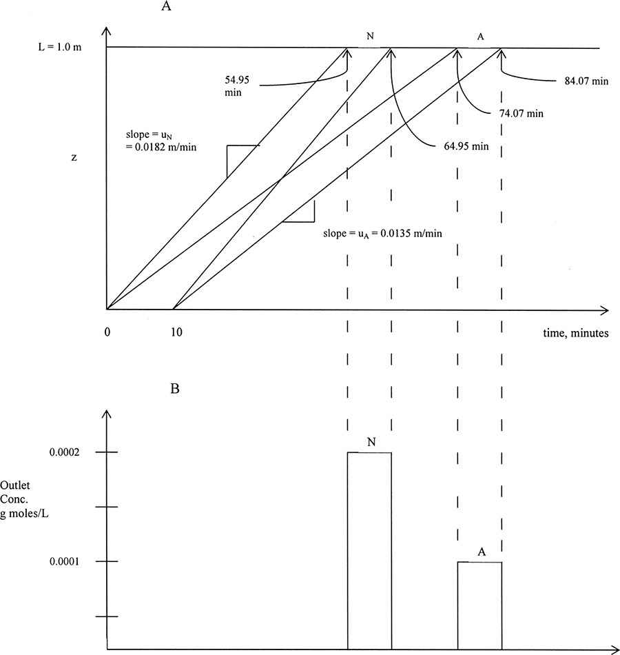
FIGURE 19-6. Results for Example 19-2 for elution chromatography; (A) solute movement diagram, (B) outlet concentration profiles
E. Check. Naphthalene input at t = 0 will exit at t = L/us,N = 1.0 m/(0.0182 m/min) = 54.95 minutes. Similarly, anthracene input at t = 0 exits at t = 74.07 minutes. Since peaks both last 10 minutes, naphthalene exits at 64.95 minutes and anthracene at 84.07 minutes. Peak centers start at tfeed/2 = 5 minutes and are at 59.95 and 79.07 minutes. These results agree with the graph in Figure 19-6A.
F. Generalize. Since no spreading phenomena are included in simple solute movement theory, outlet peaks are predicted to be square waves (Figure 19-6B). When mass transfer and axial dispersion are included, curves are spread out more, as was illustrated in Figure 19-5C. Solute movement theory correctly predicts behavior of an average molecule. Thus, times for the peak centers are correctly predicted. Dominant term in the denominator for both solutes is adsorption term (e.g., 95.3% of denominator for anthracene is from adsorption term). Adsorption will be dominant when there is relatively strong adsorption.
Basmadjian (1997) reports that a typical linear velocity for feed for liquid adsorption systems is 0.001 m/s, which is 6 cm/min. The purge velocity may be roughly ten times faster. Thus, flow rates in this problem are reasonable.
There is an analogy that may be useful in understanding solute movement analysis. Problems are similar to your high school algebra problems where two trains leave a station at same time, but with different velocities (uA and uB in chromatography). You want to calculate when each train arrives at a second station (a distance L away) and when the tail end of each train (analogous to feed time, tF) leaves the second station.
In actual practice it is much easier to calculate exit times, as shown in step E of Example 19-2, than to draw a solute movement diagram exactly to scale. Calculation of exit times can be done with a spreadsheet for much more complex processes. However, a freehand sketch of solute movement diagram should always be made, since it will guide calculations and provide a visual check on them.
In real systems results predicted by solute movement theory are spread considerably by axial dispersion, mass transfer resistances, and mixing in column dead volumes, valves, and pipes. Thus, predictions for the simple elution chromatography system shown in Figure 19-6B would spread and solute peaks would overlap, as shown in Figure 19-5C. This calculation is illustrated later in Example 19-10. If high product purities are required, zone spreading will force us to either shorten the feed step and/or lengthen the column to move peaks apart. In addition, the next feed pulse must be delayed for a considerable time, or zone spreading will result in too much overlap of slow peak with fast peak from the next feed pulse. Net result is elution chromatography can be expensive for large-scale applications. Simulated moving bed systems are often less expensive for binary separations and are analyzed in Section 19.3.3.
A number of variations of elution chromatography have been developed. In flow programming flow rate is increased to more rapidly elute the late components in Figure 19-5C. This technique does not change volume of elutant required, but reduces time of operation. Temperature programming increases temperature of the entire column during elution. Increased temperature decreases adsorption of solutes so that they exit sooner and are more concentrated. The related temperature gradient method increases temperature of fluid entering an adiabatic column. Temperature changes usually have more effect in gas systems than in liquid systems. In liquid systems it is common to use a solvent gradient to change solvent to decrease sorption of slow solutes. Common changes in solvent are to change ionic strength, polarity, pH, fraction of organic solvent, and addition of a strongly sorbed material. Gradients, which can be done as continuous changes or as step functions, are commonly used in bioseparations (Ladisch, 2001). If a solvent gradient is produced with a chemical that is more strongly sorbed than all feed components, the process is called displacement chromatography (see extensive review by Cramer and Subramanian [1990]).
A major commercial problem is purification of strongly adsorbed species such as moderate molecular weight (C10 to C20) straight-chain hydrocarbons (Ruthven, 1984). Purge systems require excessive purge gas or solvent for these strongly adsorbed species. Pressure swing cycles (Section 19.3.2) also require too much purge gas for strongly adsorbed materials. Thermal cycles (Section 19.3.1) can cause excessive thermal decomposition, since very high temperatures are required. Displacement cycles using a desorbent (e.g., n-pentane, n-hexane, and ammonia) that is adsorbed have proven to be effective for this otherwise intractable problem (Wankat, 1986). (Unfortunately, nomenclature is confusing, since displacement cycles for adsorption have a desorbent that can adsorb less or more than adsorbate, whereas in displacement chromatography the desorbent is the most strongly adsorbed compound.) Cycles will be basically the same as the counterflow cycle shown in Figure 19-5B. Since displacement adsorption requires that desorbent be recovered from product—often by distillation—they are relatively expensive processes that are used only when other adsorption processes fail. Both purge and displacement cycles are commonly used in SMB systems (Section 19.3.3).
19.3 Solute Movement Analysis for Linear Systems: Temperature and Pressure Swing Adsorption and Simulated Moving Beds
Temperature swing adsorption and pressure swing adsorption are alternative regeneration methods that can concentrate instead of dilute solute product. SMB is an alternative operating method used with purge and displacement regeneration.
19.3.1 Temperature Swing Adsorption
Temperature swing adsorption (TSA) is commonly used for gas systems, particularly for recovery or removal of trace components that are strongly adsorbed (Ruthven, 1984; Yang, 1987). Typical applications are removal of pollutants such as volatile organic compounds (VOC) (Fulker, 1972; Reynolds et al., 2002) and drying gases (Basmadjian, 1984, 1997). The basic cycle using counterflow of hot regenerant gas is shown in Figure 19-7A. A TSA cycle can be thought of as a purge operation with a hot purge gas. If feed gas flows continuously, two or more units are operated in parallel. Although pure gas is usually desired product, in some cases concentrated adsorbate is valuable. After regeneration, an optional cooling step may be inserted. Cooling is required if feed gas can react with hot adsorbent. Insertion of a cooling step tends to produce a purer product but lowers productivity (kg feed processed)/(hour × kg adsorbent).
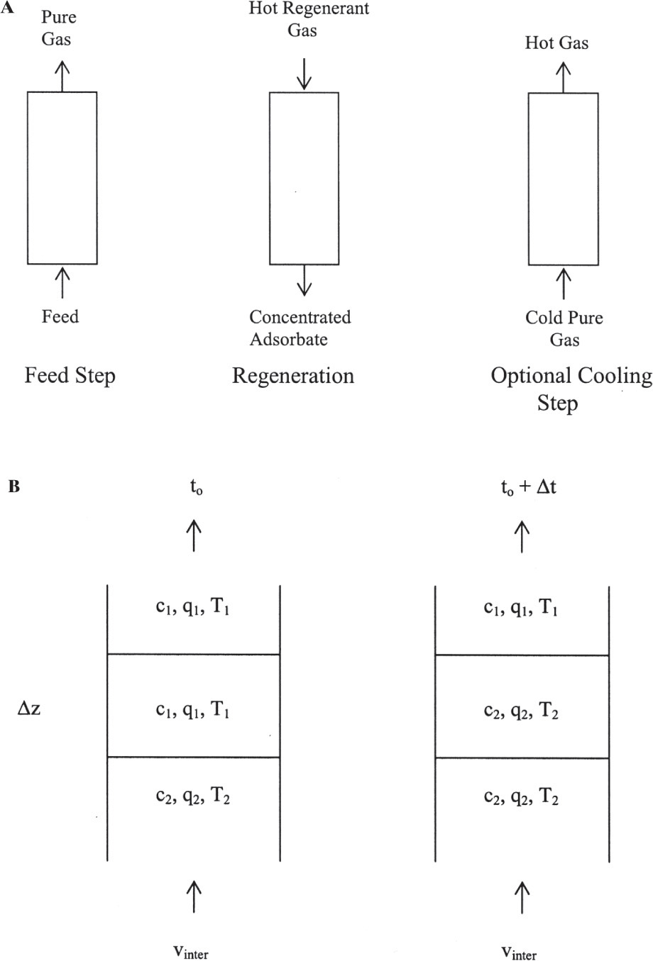
FIGURE 19-7. Thermal swing adsorption; (A) counterflow cycle for gas systems, (B) differential control volume for mass balances when temperature changes uth > us. Feed step can be done with either upward or downward flow. Part B is modified from Wankat (1986) with permission, copyright 1986, Phillip C. Wankat.
Regeneration is based on the large reduction in equilibrium observed in most adsorption systems when temperature is increased, Eq. (19-7), and simultaneous reduction in partial pressure or concentration with addition of purge gas. Both of these effects lead to removal of adsorbate. Since large increases in adsorbate concentration can occur, TSA systems are also used to concentrate dilute gas streams. When cooling is not required to prevent chemical reactions, a number of modifications have been developed (Natarajan and Wankat, 2003). These modifications are explored as homework problems.
A disadvantage of TSA systems is large amounts of pure regeneration gas may be required to heat the adsorption column and adsorbent. This occurs because at normal pressures volumetric heat capacity of gases is quite low compared to volumetric heat capacity of adsorbent and the metal column shell. Thus, regeneration is often relatively slow, expensive, and does not produce desired concentrated adsorbate product. This disadvantage tends to be minor when feed is quite dilute and adsorption is strong. Since feed period will be quite long, the relative amount of hot regenerant gas used is reasonable. However, if feed is concentrated (above a few percent), adsorbent will saturate fairly quickly and feed period will be relatively short. Since the same amount of hot regenerant gas is required to heat the column, ratio (hot regenerant gas/feed gas) can become excessive.
To study TSA systems with solute movement analysis we must determine (1) effect of temperature changes on solute waves, (2) rate at which a temperature wave moves in column, and (3) effect of temperature changes on concentration. The first of these is easy. As temperature increases equilibrium constants, KA and K′A both decrease, often following an Arrhenius relationship, as shown in Eq. (19-7). If effect of temperature on equilibrium constants is known, new values of equilibrium constants can be calculated and new solute velocities can be determined.
Changing temperature of feed to a packed column will cause a thermal wave to pass through the column. Velocity of this thermal wave can be calculated by a procedure analogous to that used for solute waves. Thermal wave velocity will be fraction of change in thermal energy in mobile phase multiplied by interstitial velocity:
Since changes in energy contained in fluid in pores, in solid, and in walls are stagnant, this fraction is

In this derivation we assume a pure thermal wave with no adsorption, no reactions, and no phase changes. Thus, energy changes are totally due to specific heat. For example, amount of energy change in mobile phase is
where CP,f is fluid heat capacity and ΔTf is fluid temperature change. Substituting in appropriate terms, fraction of energy change in mobile phase is

where W is column weight per length (kg/m), and ΔTpf, ΔTs, and ΔTw are changes in pore fluid, solid, and wall temperatures induced by the change in fluid temperature. If we divide numerator and denominator of Eq. (19-19) by ΔTf, we have ratios of ΔTpf, ΔTs, and ΔTw to ΔTf. If heat transfer is very rapid, the system is in thermal equilibrium, Tf = Tpf = Ts = Tw. This equality requires that changes in temperature all be equal:
and ratios of changes in temperatures are all one. Combining Eqs. (19-17), (19-19), and (19-20), the resulting thermal wave velocity is
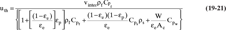
As a first approximation, thermal wave velocity is independent of concentration and temperature. Temperature is constant along lines with slope = uth.
In TSA processes temperature is increased to remove adsorbate from adsorbent. This happens when thermal and solute waves intersect. The column is initially at a uniform temperature T1, concentration c1, and adsorbent loading q1. Fluid at temperature T2 is fed into the column. This temperature change causes concentration and adsorbent loading to change to c2 and q2 (currently both unknown). Since solute movement theory assumes local equilibrium, c2 and q2 are in equilibrium at T2. The control volume shown in Figure 19-7B (Wankat, 1986) will be used to develop the mass balance for this temperature change. Initially, the thermal wave is at the bottom of the control volume. Thermal waves are assumed to move faster than solute waves, which is true for most dilute liquid and some dilute gas systems. For a differential slice of column of arbitrary height Δz, temperature of the slice will change from initial temperature T1 to final temperature T2 if Δt = Δz/uth. The mass balance for the differential slice over time interval Δt is
Since Δt = Δz/uth, this simplifies to

Equation (19-23) and the isotherm equation can be solved simultaneously for the unknowns c2 and q2. For a linear isotherm, Eq. (19-6b), simultaneous solution is

Example 19-3 illustrates that for liquid systems with uth > us, use of a hot feed liquid (T2 > T1) will increase outlet concentration.
EXAMPLE 19-3. Thermal regeneration with linear isotherm
Use a thermal swing adsorption process to remove traces of xylene from liquid n-heptane using silica gel as adsorbent. The adsorber operates at 1.0 atm. Feed is 0.0009 wt% xylene and 0.9991 wt% n-heptane at 0°C. Superficial velocity of feed is 8.0 cm/min. Adsorber is 1.2 meters long and during feed step is at 0°C. Feed is continued until xylene breakthrough occurs. Regeneration is done with counterflow of pure n-heptane at 80°C continued until all xylene is removed. Superficial velocity during purge is 11.0 cm/min.
Data: At low concentrations isotherms for xylene: q = 22.36x at 0°C, q = 2.01x at 80°C, q and x are in g solute/g adsorbent and g solute/g fluid, respectively (Matz and Knaebel, 1991). ρs = 2100 kg/m3, ρf = 684 kg/m3, Cps = 920 J/kg °C, Cpf = 1841 J/kg °C, εe = 0.43, εp = 0.48, Kd = 1.0.
Assume: Since column diameter is large, W/Ac is small and wall heat capacity can be ignored, heat of adsorption is negligible, no adsorption of n-heptane, and operation with repeated feed pulses is at cyclic steady state.
Use solute movement theory to determine
A. Breakthrough time for xylene during the feed step.
B. Time for thermal wave to breakthrough during both feed and purge steps.
C. Xylene outlet concentration profile during purge step.
Solution
A. Define. Process is similar to sketch in Figure 19-7A but without optional cooling step. Breakthrough time for solute is time that xylene first appears at column outlet, z = L. thermal wave breakthrough times occur when temperature starts to decrease (during feed step) or increase (during purge step). Desired outlet concentration profile is xylene concentration versus time.
B. Explore. Since operation is at cyclic steady state (each cycle is an exact repeat of previous cycle), column will be hot when cold feed is started. Cold feed causes a cold thermal wave during the feed step. We expect that this wave will move faster than xylene wave (this expectation will be checked while doing calculations); thus, waves are independent. When flow direction is reversed, xylene wave concentration is unchanged until thermal wave intersects xylene wave. Because temperature changes in the column are not instantaneous, there is a period when liquid exiting from the column bottom is at the feed concentration (study Figure 19-8 to understand this). When the two waves intersect, temperature increases, isotherm parameters decrease, and xylene wave velocity increases. At the same time, xylene is desorbed and xylene concentration in fluid increases.
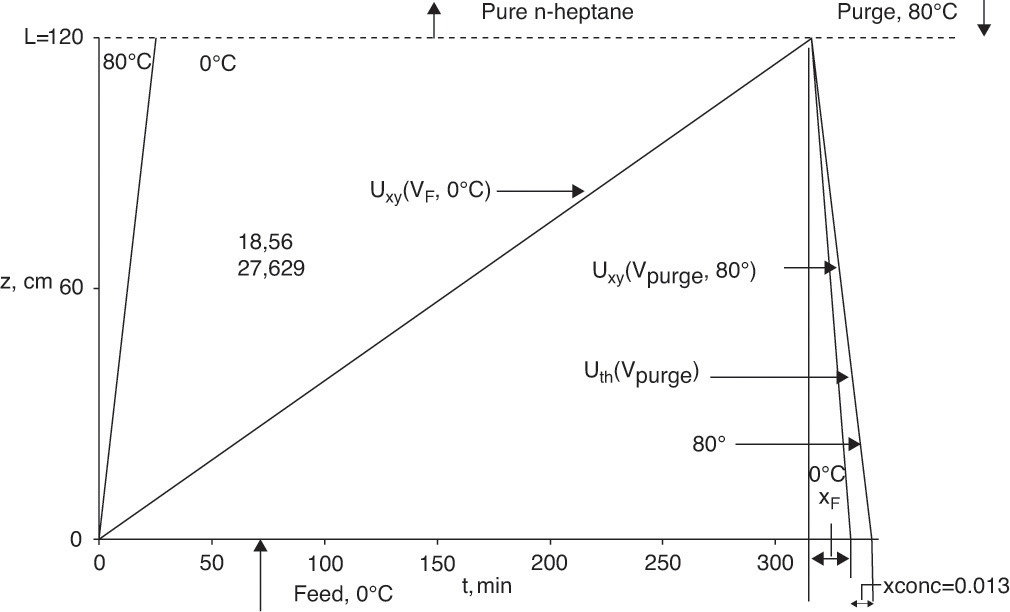
FIGURE 19-8. Solute movement solution for counterflow TSA in Example 19-3
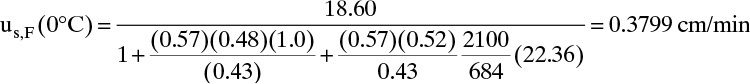
C. Plan. Since mass fractions are used in equilibrium expression, we use Eq. (19-15c) to calculate velocity of solute at 0°C and 80°C. Thermal wave velocity is determined from Eq. (19-21) with W = 0. Effect of temperature change on fluid concentration can be determined either from a mass balance over one cycle or from Eq. (19-24).
D. Do it.
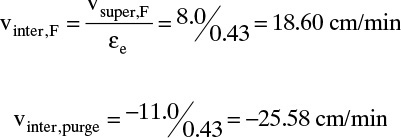
To calculate solute velocity during the feed step use Eq. (19-15c):
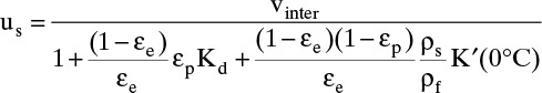
At 0°C, K′ (0°C) = 22.36 g xylene/g adsorbent. Then,
And xylene breakthrough time is
Thermal wave velocity from Eq. (19-24) with W term = 0 is
And thermal breakthrough time is ![]() .
.
During purge step, vinter,purge = –25.58 cm/min and uth,purge = –9.494 cm/min. They are negative because the flow direction is reversed. Breakthrough time is
Note that thermal wave moves considerably faster than solute wave and thus breakthrough is quicker. After temperature change, K′ (80°C) = 2.01, and solute velocity and breakthrough time during purge are
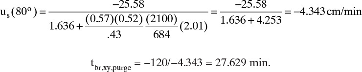
Xylene mass balance on one cycle at cyclic steady state is In = Out.
In (8.0 cm/min)(Ac, cm2)(315.85min)ρf (g solv cm3)(0.0009 g xylene/g soln)
The outlet stream shown in Figure 19-8 consists of one part at xF and one part that is concentrated at unknown mass fraction xconc.
(11.0 cm/min)(Ac,cm2)(12.64 min)(ρf g solvent/cm3)(0.0009 g xylene/g soln)
+ (11.0 cm/min) (Accm2)(27.629 – 12.64 min)(ρf g solvent/cm3)(xconc)
Set In = Out, divide out Ac and ρf (assumed to be constant), and solve for xconc:

Xylene exiting the column bottom is at xout = xF = 0.0009 for the first 12.64 minutes of regeneration step. Then from 12.64 to 27.629 minutes of regeneration, xout = xconc = 0.013. If regeneration continues for times longer than 27.629 minutes, xout = 0. Average weight fraction during 27.629 minutes of regeneration is xout,avg = 0.00746.
E. Check. Equation (19-24) can be used to check outlet xylene weight fraction. This equation is applied at the point where the adsorbent changes temperature during the purge step; thus, all velocities should be calculated at purge velocity. Since solute velocity is directly proportional to interstitial velocity,
us(vpurge, T = 0) = us(vF, T = 0) (vpurge/vF) = (0.3799)(–11.0/8.0) = –0.5224 cm/min.
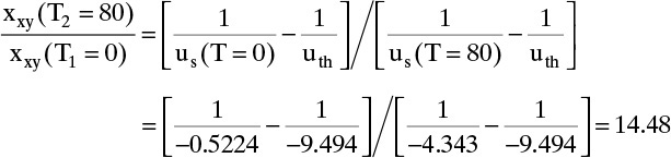
xxy (T = 80°C) = (14.48)(0.0009) = 0.013, which checks mass balance result.
F. Generalize. The increase in solute concentration during thermal regeneration is a general phenomenon for strongly adsorbed solutes if feed is dilute. Even more concentration can be obtained by recycling material at feed concentration that exits during the purge step. Energy required to concentrate dilute xylene in n-heptane by adsorption is significantly less than energy required to do the same concentration by distillation. (Going from 0.0009 wt% to 0.013 wt% xylene may not seem like much change, but removal of a very large amount of pure n-heptane is necessary to obtain this amount of concentration.)
If solute waves move faster than thermal waves, which may occur in dilute gas systems, a mass balance equation and solution similar but subtly different from Eqs. (19-22) to (19-24) can be derived. In this situation concentrated solute exits ahead of the thermal wave instead of behind it, as predicted by Eqs. (19-22) to (19-24). One other case that can occur but is rare in dilute systems is when us(Thot) > uth > us(Tcold). In this case, which is not included in this introductory treatment, solute concentrates, or focuses, at the temperature boundary (Wankat, 1990).
A number of different thermal cycles are used commercially. Figure 19-9 shows an alternate TSA cycle commonly used for recovery of solvents (typically volatile organic compounds (VOC) of intermediate molecular weight ∼45 to 200) from drying and curing operations (Basmadjian, 1997; Fulker, 1972; Wankat, 1986). Activated carbon is used as adsorbent, and steam is used as regeneration gas. Horizontal beds with a depth of 1 to 2 meters are often employed, since strong adsorption of solvent on activated carbon allows for quite short beds, and large gas flows require a large cross-sectional area to avoid excessive pressure drop. If feed gas needs to be treated continuously, two or more adsorbers are used in parallel, with a typical feed time of approximately 2 hours. Because latent heat of steam is high, a large amount of energy can be rapidly transferred into the adsorber, heating it quickly. A “heel” of leftover solvent is usually left in the bed, since complete regeneration of the bed would require excessive amounts of steam. Because of incomplete regeneration and competition with water vapor for adsorption sites, typical design capacity used for activated carbon is about 25% to 30% of maximum carbon capacity. Bed capacity can be increased by reducing relative humidity of feed gas to less than 50%.
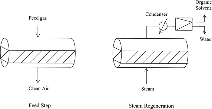
In ideal applications of this process (e.g., removing small amounts of toluene from air), peak mole fractions of toluene are close to 1.0 (Basmadjian, 1997) and toluene is almost completely immiscible with water. Thus adsorbate can be recovered from the exiting regeneration vapor by condensing the vapor and allowing liquid to separate into an organic layer and a water layer. If adsorbate is miscible with water (e.g., ethanol), the condenser/settler shown in Figure 19-9 must be replaced with a distillation column, which greatly increases capital and operating costs.
Note that there can be safety hazards in operation of activated carbon solvent recovery equipment (Figure 19-9). If solvent being recovered is flammable, care must be taken to prevent a fire. If feed gas is air, then concentration of solvent in feed gas must be kept below lower explosion limit, and is often kept below one-quarter of lower explosion limit to provide a safety margin. This requirement invariably means that feed gas must be quite dilute and flow rates are large. If feed gas is hot, it is often cooled before the adsorber to increase safety and to increase adsorption capacity. An alternative is to operate at much higher concentrations using nitrogen or carbon dioxide as carrier gas, but then carrier gas must be recovered and recycled. If hot activated carbon can catalyze a reaction with feed, a cooling step is added. Sometimes a drying step is added before cooling, since water may interfere with adsorption or react with feed. If feed gas is concentrated, adsorbent can become quite hot because of the large heat of adsorption. Unfortunately, carbon beds occasionally catch fire when this happens. Fire can be prevented by significant cooling of feed gas, incorporating a cooling step in the cycle, or replacing air with an inert gas.
Since several companies provide package units for activated carbon solvent recovery, new engineers are more likely to be involved in purchase and installation of a unit than in designing a new unit. The more you know about solvent recovery with activated carbon, the better choice of unit and better bargain you will be able to make for your company.
Various thermal cycles are also employed for liquid systems, although they tend to be somewhat different than those used for gases. The largest application of liquid adsorption is the use of activated carbon to treat drinking water and wastewater (Faust and Aly, 1987). Since contaminant levels are very low and adsorption tends to be very strong, feed may last for several months. Regeneration of activated carbon is difficult and is usually done by removing carbon from the column and sending it to a kiln to burn off adsorbates. In small units (e.g., those used to purify tap water in homes) carbon is discarded after use. Activated carbon is commonly used in bottling plants to remove chlorine from water by reacting with carbon to produce HCl (Wankat, 1990). The slightly acidic water should be used immediately after treatment, since it no longer contains chlorine to stop microbial growth.
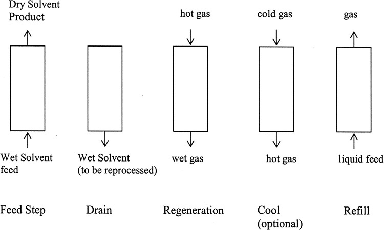
A major industrial application of liquid adsorption is drying of organic solvents, shown in Figure 19-10 (Basmadjian, 1984). Upward flow is used during refilling and feed steps to avoid trapping gas in the bed. Since water content in the organic is usually low, the feed step may be relatively long. Once breakthrough occurs (substantial amounts of water appear in exiting solvent), feed is turned off and the column is drained. Regeneration is done with downward flow of hot gas and is usually followed by a cooling step. Adsorptive drying competes with drying by distillation (Chapter 8). Operating expenses for adsorptive drying are dominated by cost of energy to evaporate residual liquid and desorb water. Adsorptive drying usually is less expensive than distillation when water concentrations in solvent are low.
In concentrated systems energy generated by adsorption can be as large as or significantly larger than the sensible heat from the temperature change. This causes a coupling of concentration and temperature waves, and they often travel together. Basmadjian (1997) presents a simple way to estimate maximum temperature rise.
Typical range for heat of adsorption |ΔHads| is from 1000 to 4000 kJ/kg (average ∼2500), and typically gas heat capacity CP,f is approximately 1.0 kJ/kg. This estimate gives a maximum temperature rise of approximately 25°C for a feed containing 1.0 wt% adsorbate and a maximum temperature rise of 1.25°C for a feed containing 0.05 wt% adsorbate. Basmadjian (1997) states an isothermal analysis can be used if predicted maximum temperature increase is less than 1°C or 2°C. Situations with large temperature increases are economically important, but detailed theoretical treatment is beyond the scope of this introductory chapter. Interested readers should consult Basmadjian (1997), LeVan et al. (1997), Ruthven (1984), or Yang (1987). These more concentrated systems can also be simulated with commercial simulators.
19.3.2 Pressure Swing Adsorption
Pressure swing adsorption (PSA) and vacuum swing adsorption (VSA) cycles are alternatives to thermal cycles for gas systems. They are particularly useful for more concentrated feeds and/or adsorbates that are not strongly adsorbed. Figure 19-11A shows steps in the basic Skarstrom cycle (named after Charles Skarstrom, the process inventor) for PSA (Ruthven et al., 1994; Wankat, 1986). Usually, desired product is pure product gas after adsorbate removal. Typical applications include drying gases, purifying hydrogen, and producing oxygen or nitrogen from air.
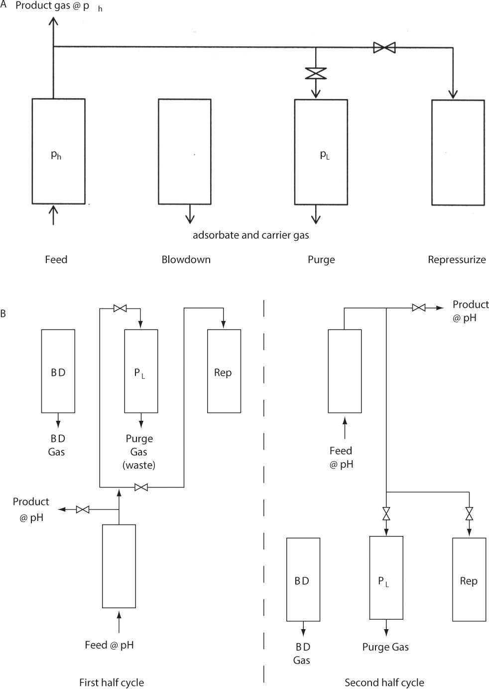
FIGURE 19-11. Pressure swing adsorption; (A) steps for single column in Skarstrom cycle, (B) use of two columns in parallel for continuous feed and product. BD = blowdown, Rep = repressurization. Period of feed step = period of blowdown + purge + repressurization steps.
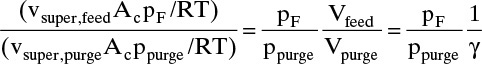
Following a relatively high pressure feed step, column pressure is reduced to a lower pressure by counterflow blowdown. At this reduced pressure the column is purged (counterflow to feed) using part of the pure product gas. Since pure product gas is used as a purge, purge product (or waste) gas contains both adsorbate and carrier gas. Volume of purge gas required for the Skarstrom cycle is
where γ typically is between 1.15 and 1.5. Because of volumetric expansion of product gas from ph to purge gas at pL, significantly fewer moles of purge gas are needed than feed gas. Dropping pressure also reduces partial pressure, which helps desorb adsorbate. The final step in the Skarstrom cycle is column repressurization. This step was originally done with fresh feed gas, although with concentrated systems it is now much more common to use high-pressure product gas, as shown in Figure 19-11. Usually two or more columns are operated in parallel, but with cycles out of phase so that one column is producing product when the other needs to be purged or repressurized. One method of doing this is shown in Figure 19-11B. PSA systems with from 1 to 12 columns are used commercially. PSA has fast cycles—a minute or two is common in industry, and some cycles are as short as a few seconds. Short cycles lead to high productivity and hence relatively small adsorbers.
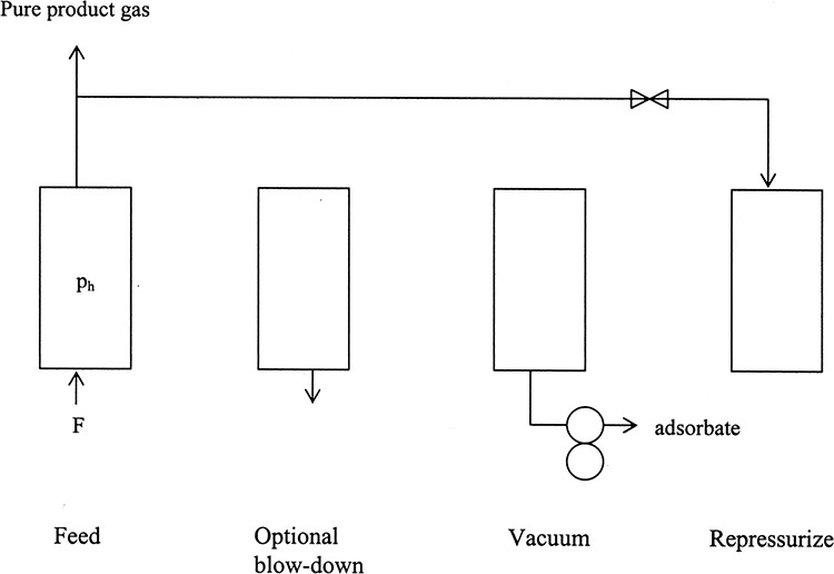
Figure 19-12 illustrates a simple vacuum swing cycle. Feed enters at high pressure, which may be essentially atmospheric pressure. If ph is significantly above atmospheric pressure, a short optional blowdown step can be included. A vacuum pump is used to reduce pressure to very low pressures. At very low pressures, partial pressure is very low and very little adsorbate can be adsorbed (see Figure 19-2). Unfortunately, this step is slow, and productivities of VSA systems are low. However, VSA has the advantage that a relatively pure product gas and a relatively pure adsorbate product can be produced. For example, VSA units can separate air into an oxygen product and a nitrogen product. The final step is column repressurization. VSA units are usually operated with several columns in parallel. A large number of variations of PSA, VSA, and combinations of PSA and VSA cycles have been invented (Kumar, 1996; Ruthven et al., 1994). For example, it is common to operate PSA purge at a pressure less than atmospheric.
Simple Skarstrom PSA cycles (Figure 19-11A) have constant pressure (isobaric) periods and periods when pressure is changing. We will assume that a very dilute gas stream containing trace amounts of adsorbate A in a weakly adsorbed carrier gas is being processed, and equilibrium is linear over the concentration range of interest. If mass transfer is very rapid, then solute movement theory can be applied. Since system is very dilute, the system is assumed to be isothermal and gas velocity is constant. In more concentrated PSA systems neither of these assumptions is true, and more complicated theories or complete simulations must be used (Ruthven et al., 1994).
During isobaric periods (feed at ph and purge at pL), solute moves at a velocity us. For an ideal gas and a linear isotherm in partial pressure units, solute velocity is given by Eq. (19-15d). Normally, Kd,i = 1.0 and all adsorption sites are accessible to small gas molecules.
During blowdown, mole fraction of adsorbate increases because of desorption as pressure drops. During repressurization the opposite occurs and adsorbate mole fraction in gas decreases. When pressure changes, solute waves shift locations. Determining mole fraction changes and shifts in location for these steps requires solution of partial differential equations (Chan et al., 1981). Results for linear isotherms are relatively simple. Define parameter βstrong for the strongly adsorbed component as

This parameter is ratio of the amount of weakly adsorbed to the amount of strongly adsorbed adsorbate in a column segment. If weakly adsorbed component does not adsorb, then ![]() in Eq. (19-27). Since
in Eq. (19-27). Since ![]() , βstrong < 1.0. The shift in mole fraction of strongly adsorbed species A when pressure changes is
, βstrong < 1.0. The shift in mole fraction of strongly adsorbed species A when pressure changes is
Equation (19-28a) predicts an increase in mole fraction yA for a decrease in pressure (try it to convince yourself). The shift in location of solute waves can be found from
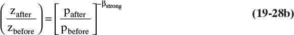
where axial distance z must be measured from closed column end (closed end can vary during PSA cycles). Note that if zbefore = 0, then zafter = 0. Solute waves at the closed column end cannot shift.
Application of solute movement theory is illustrated in Example 19-4. Before doing this activity, we note that axial dispersion is normally significant in gas systems. Thus we expect solute movement theory will overpredict separation that occurs. Alternatively, γ required in Eq. (19-26) for a given product purity will be larger in a real system than predicted by solute movement theory (γ = 1 for linear systems). For separations based on differences in equilibrium isotherms, if solute movement theory predicts a separation is not feasible or will not be economical, more detailed calculations will rarely improve results.
A 0.50 m long column is used to remove methane (M) from hydrogen using Calgon Carbon PCB activated carbon. Feed gas contains 0.002 mol% methane. Superficial velocity is 0.0465 m/s during feed step. High pressure is 3.0 atm, and low pressure is 0.5 atm. A standard 2-column Skarstrom cycle is used. The symmetric cycle is
Repressurize with feed 0 to 1 s.
Feed step at pH 1 to 30 s.
Purge at pL 31 to 60 s.
Operation is at 480 K. Use a pure purge gas with a purge to feed ratio of γ = 1.1. Carbon properties: ρs = 2.1 g/cc, Kd = 1.0, εp = 0.336, εe = 0.43. Equilibrium data are available in Table 19-3 and has been analyzed in Example 19-1. Draw a diagram for the first cycle assuming the bed is initially clean at 0.5 atm, and predict the outlet concentration profile.
Solution
A. Define. Plot movement of solute during the four steps shown in Figure 19-11A, and use this diagram plus appropriate equations to predict outlet mole fractions.
B. Explore. The Arrhenius plot table in Example 19-1 gives KM = 1.888 × 10⁻⁴ (kPa)–1 and qmax = 3.84 mmol/g at 480 K. Since feed mole fraction is very low, isotherm will be in linear range ![]() where
where ![]() = qmaxKM = (3.84) (1.888 × 10⁻⁴) = 0.000725 mmol/(K g Pa). Since hydrogen does not adsorb,
= qmaxKM = (3.84) (1.888 × 10⁻⁴) = 0.000725 mmol/(K g Pa). Since hydrogen does not adsorb, ![]() . We will assume operation is isothermal.
. We will assume operation is isothermal.
C. Plan. Start by repressurizing with feed. We can calculate βM from Eq. (19-27) and distance wave moves in the column can be determined from Eq. (19-28b). During feed step at 3.0 atm, methane travels at a constant solute velocity given by Eq. (19-15d). There will be two waves, as shown in Figure 19-13A. During blowdown, Eq. (19-28a) is used to determine the new mole fraction. Waves during the purge step again follow Eq. (19-15d) but with vpurge = γ vfeed.
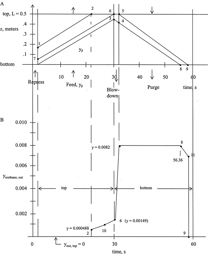
FIGURE 19-13. Solute movement solution for PSA system in Example 19-4; (A) solute movement diagram, (B) outlet concentration profiles
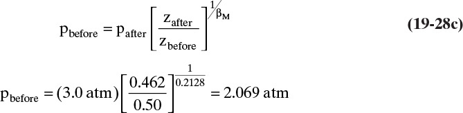
D. Do it. Repressurization Step: From Eq. (19-27),
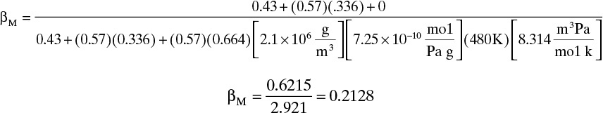
Units of the last term in the denominator are a little tricky. The gas constant used is R = 8.314 m3Pa/(mol K). If a different gas constant is used, units on other terms have to be adjusted.
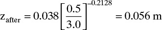
Equation (19-28b) is used for shift in location of solute waves. Because the column top in Figure 19-11A is closed, z is measured for this step from that end. Then the feed end is at z = 0.50 m. From Eq. (1-28b)
This is 0.50 – 0.3415 = 0.1585 m from the feed end of the column (point 1 in Fig. 19-13A). Mole fraction methane at this location can be determined from Eq. (19-28a):
where yM, before = 0.002 is feed mole fraction from column bottom which shifts during repressurization to point 1. Mole fraction yM, after is lower since methane is adsorbed as column is pressurized.
Feed Step: Equation (19-15d) is used to determine methane solute velocity uM:

(Note the denominator is the same as the denominator for βM.)
Since εevinter = vsuper = 0.0465 m/s, ![]()
During the 29 seconds of the feed step, methane waves can move 0.462 m. Thus one methane wave breaks through while the other does not (see points 2 and 3 on Figure 19-13A).
The wave that breaks through travels 0.3415 m, which requires (0.3415 m)/(0.01592 m/s) = 21.45 s. Including 1.0 seconds for repressurization, this is 22.45 s after start of the cycle. Point 3 is at z = 0.462 m.
Blowdown: Point 3 will shift according to Eq. (19-28b) with the closed end again at the top. Thus, measuring from top we have
zbefore = 0.5 – 0.462 = 0.038 m
and from Eq. (19-28b)
or 0.50 – 0.056 = 0.444 m from the bottom. With ybefore = yF = 0.002, Eq. (19-28a) gives
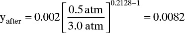
As expected, methane mole fraction increases as methane desorbs.
Purge Step. Methane velocity during purge is again given by Eq. (19-15d); however, interstitial velocity is increased, since γ > 1.0.
vsuper, purge = γ vsuper, feed = (1.1)(0.0465) = 0.05115 m/s
Then
uM, purge = γ uM, feed = (1.1)(0.01592) = 0.01751 m/s
There are two waves (from top of column, point 5, and from point 4). They can both travel 0.508 m in 29 s; thus they both exit the column.
Wave from point 4 exit time: 0.444 m/(0.01751 m/s) + 31 s = 56.36 s (point 8)
Wave from point 5 exit time: 0.5 m/(0.01751 m/s) + 31 s = 59.57 s (point 9)
Outlet Mole Fraction Profile: At the top of the column:
0 to 1 s, no product
1 to 22.45 s (point 2), y = 0
At point 2, y = 0.000488
At point 6, to estimate mole fraction, follow solute back to point 7 at t = 1 s (end of repressurization).
z7 = tfeed/uM, feed = (29 s)(0.01592 m/s) = 0.462 m from top
Final mole fraction at point 7 follows solute that enters during repressurization at a specific, but unknown, pressure between pL = 0.5 and pH = 3.0 atm. Equation (19-28b) can be employed with zafter = 0.462, zbefore = 0.50, pafter = 3.0, βM = 0.2128 to calculate this unknown pressure, pbefore. Then
Since feed entered at yM, before = 0.002, Eq. (19-28a) can be used to estimate yM, after:
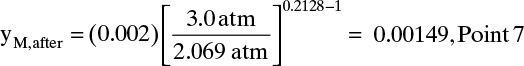
Since concentrations are constant along the trace of solute movement, this is mole fraction at point 6. A similar procedure can be used (see Problem 19.D10) to find intermediate point 10 (shown at 26.126 s and yM = 0.000876). Outlet profile is not linear.
During blowdown, gas exits (at bottom of column) initially at yF = 0.002 and increases to yafter, BD = 0.0082. Profile shape can be estimated by the procedure used above. Mole fraction is constant at 0.0082 until gas from point 4 exits at point 8 at 56.36 s. Gas mole fraction drops to yout = 0, and the column is completely regenerated at point 9 (59.57 s). Intermediate point 11, shown in Figure 19-13B, is estimated (see Problem 19.D10).
E. Check. Because flow rates vary in unknown ways during repressurization and blowdown steps, a complete mass balance check is not possible. However, an approximate check balancing methane flows in feed and purge steps can be done.
Methane during feed = vsuper,feedAcyM,F ρm,FtF = vsuperAcyM,FtFpF/RT
where the molar density is ρm,F = pF/RT for an ideal gas and Ac = cross-sectional area.
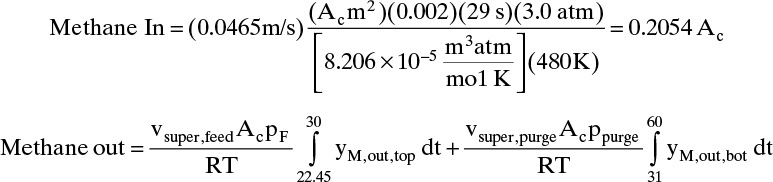
The integrals can be estimated by assuming variation in yM is linear:
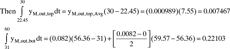

The inlet and outlet amounts are reasonably close.
F. Generalization Notes:
1. Ratio of moles gas fed to purge gas used:
is ![]() and (ignoring repressurization and blowdown) ratio of product gas (hydrogen) to feed gas is
and (ignoring repressurization and blowdown) ratio of product gas (hydrogen) to feed gas is

PSA produces a significant amount of high-pressure pure product because gas is expanded before it is used for purging.
2. This design is inappropriate if pure hydrogen is desired during the entire feed step. Breakthrough can be prevented by changing the design (see Problem 19.B2).
3. Repressurization with feed causes methane to penetrate the bed a significant distance during this step. Repressurization with product works better (see Problem 19.D11).
4. This example uses complete regeneration (column is clean at end of cycle). Incomplete regeneration (leaving a heel) increases pure product production and is employed in industrial systems.
This section illustrated PSA calculations for the simplest possible case—local equilibrium theory for trace components for an isothermal system. If feed mole fraction of strongly adsorbed component is higher, velocity will vary in the column, and the isotherm is probably nonlinear. In addition, operation is much more likely to be adiabatic instead of isothermal. It is also common to have both components adsorb or to have more than two components. If dispersion and mass transfer resistances are important, detailed simulations are required. Ruthven et al. (1994) provide an advanced treatment. In addition, PSA has spawned a large number of inventive cycles to accomplish different purposes. White and Barkley (1989) and White (2008) discuss practical aspects of PSA design, such as pressure drops, velocity limit to prevent bed fluidization, retaining heat of adsorption in the bed, and start-up.
19.3.3 Simulated Moving Beds
Most adsorption processes remove all adsorbed solutes from a nonadsorbed or weakly adsorbed carrier gas or solvent. Elution chromatography, on the other hand, was developed to separate a number of solutes from each other with all products containing carrier gas or solvent. Simulated moving bed (SMB) technology is a melding of purge or displacement adsorption and chromatographic methods that was developed by UOP in late 1950s and early 1960s (Broughton and Gerhold, 1961; Broughton et al., 1970). SMBs are currently extensively used for binary separations. Although gas-phase systems have been studied, all current commercial applications are liquid-phase (see Problem 19.A6). Common industrial applications of SMBs are separation of aqueous solutions of glucose from fructose to make sweeteners (heavily used in soft drinks), separation of p-xylene (used to make polyesters) from m-xylene, and separation of optical isomers in the pharmaceutical industry. The SMB process is relatively expensive, since products must be separated from solvent or desorbent usually by evaporation or distillation (Ruthven, 1984; Wankat, 1986).
The most efficient approach to separating a binary mixture by adsorption appears to be to have a countercurrent process similar to extraction. In addition, it is convenient to regenerate adsorbent within the device. True moving bed (TMB) systems (Figure 19-14A) were invented to achieve these two goals. Zones 2 and 3 separate the two solutes. (Zones are packed regions between inlet and outlet ports.) Zone 1, which is optional but almost always included, adsorbs weakly adsorbed solute A onto solid so that desorbent D can be recycled. Zone 4 regenerates solid by removing strongly adsorbed solute B using a purge or displacement with desorbent D. Figure 19-14A is loosely analogous to distillation: A is light key, B is heavy key, zones 2 and 3 are enriching and stripping sections, respectively; and zones 1 and 4 are analogous to a total condenser and a total reboiler, respectively. TMB systems would work if chemical engineers had technology to build large-scale systems that could move a solid countercurrent to a fluid with no axial mixing. Since this goal has proved to be elusive, UOP developed the SMB.
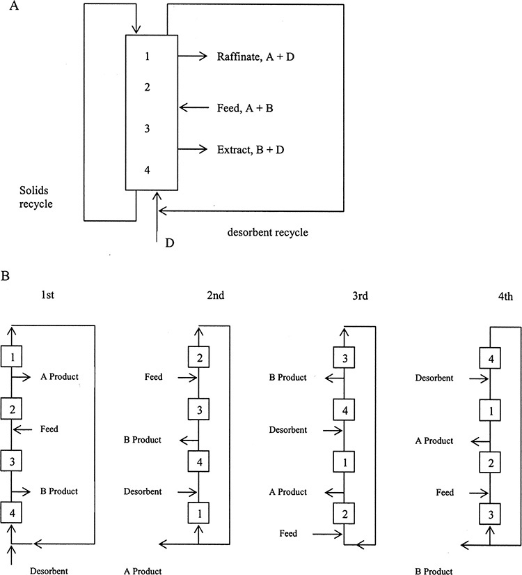
FIGURE 19-14. Separation of binary mixtures by adsorption; (A) TMB, (B) SMB showing complete cycle with four columns and four time steps
An SMB system is shown in Figure 19-14B for four different time steps. SMB columns are arranged in a continuous loop with inlet and outlet ports. After a set time period, switching time tsw, port locations are all advanced by one column. From the viewpoint of an observer at the extract port, solid moves downward when the switch is done while fluid continues to move continuously upwards. Thus an intermittent, countercurrent movement of solid and liquid has been simulated. Port switching is continued indefinitely. In Figure 19-14B with four columns, the cycle repeats after every four switches. If there are N columns, the cycle repeats after N switches. A large number of modifications to SMBs have been developed. Most common is to have two or more columns per zone instead of one column per zone, shown in Figure 19-14B. This makes operation closer to a TMB and improves the product purity.
The SMB system shown in Figure 19-14B is quite a complicated system, particularly if compared to simple elution chromatography shown in Figure 19-5B. Chin and Wang (2004) discuss practical aspects of SMB systems, such as pump placement, pressure drops, and valve requirements. SMBs are used in industry for high-purity separations of binary feeds, since much less desorbent and adsorbent are required. Solute movement analysis helps to explain how this complicated process works.
Each column in Figure 19-14B is a chromatographic column. Port switching changes flow rate and boundary conditions for each column. Solute velocity in each SMB column can be determined in the same way as for elution chromatography. Thus solute velocity in any SMB column is given by Eqs. (19-15). Chromatography and SMB processes differ only in column coupling, which are boundary conditions!
To separate solutes A and B completely, SMBs must meet the following conditions:
Zone 1. To produce pure desorbent for recycle, solute A must not breakthrough (that is, appear in outlet of zone 1) during switching period, tsw. Thus
uA,1 tsw ≤ L
Since average port velocity is defined as uport = L/tsw, this condition becomes
Equations are written as equalites instead of inequalities, since it is easier to manipulate equations.
Zones 2 and 3. To separate A and B we want net movement of A upward and net movement of B downward in the column. Since velocity is higher in zone 2, the condition on solute B controls.
In zone 3 upward movement of solute A controls.
These conditions require that solute A break through and solute B not break through from zones 2 and 3 during a switching period.
Zone 4. To regenerate, all solute B must be removed in zone 4; thus solute B must have net upward movement.
Equations (19-29a) to (19-29d) can be simultaneously satisfied by changing flow rates of feed, desorbent, and two product streams in Figure 19-14B to change velocities in each zone. For example, since A product stream is withdrawn between zones 1 and 2, v1 < v2. By proper selection of velocities and port velocity, we can satisfy these four equations (see Example 19-5).
Usually desorbent must be removed from A and B product streams. Increasing desorbent flow rate increases cost for removal and will also increase column diameters and require more adsorbent. Thus desorbent to feed ratio, D/F, often controls SMB system cost. For an ideal system with no zone spreading (no axial dispersion and very fast mass transfer rates), solute movement theory can be used to calculate D/F by solving Eqs. (19-29a) to (19-29d) simultaneously with Eq. (19-15) and mixing mass balances with constant density.
where vFeed = F/(εe Ac) is the interstitial velocity that feed would have in the column. F is volumetric flow rate of feed, and Ac is the cross-sectional area of columns with similar definitions for desorbent and product velocities. If F and Ac are known, we can first solve for uport, v1, v2, v3, and v4, then for vA,product, vB,product, and vD, and finally D/F = vD /vFeed. These calculations are developed in Problem 19.C10. Minimum D/F ratio, (D/F)min can be calculated by setting all Mi = 1.0. This minimum has significance similar to that of (L/D)min in distillation. For linear systems (D/F)min = 1.0, which is also the thermodynamic minimum.
In practice there is considerable spreading due to mass transfer resistances, axial dispersion, and mixing in transfer lines and valves. If an SMB is operated at (D/F)min, raffinate and extract products will not be pure. To obtain higher purities, D/F is usually increased; however, SMBs are more complicated than binary distillation. The additional desorbent must be distributed throughout four zones to give optimum velocities in each zone. One optimization approach is to pick values of multipliers M1 < 1, M2 < 1, M3 > 1, and M4 > 1. Then velocities and D/F can be determined by solving the solute movement equations (see Problem 19.C10 for equation for D/F). The experiment or simulation is then run again with these new flow rates. The procedure is repeated until desired purities are achieved.
Design an SMB system to separate fructose and glucose. Ching and Ruthven (1985) found that equilibrium of fructose and glucose on ion exchange resin in calcium form was linear for concentrations below 5 g/100 ml. Their equilibrium expressions are qgluc = 0.51 cgluc, qfruc = 0.88 cfruc, at 30°C with both q and c in g/L. If switching time tsw = 5 min and Dcol = 0.4743 m, design an SMB system with one column per zone at minimum D/F = 1.0. Data: εp = 0 and εe = 0.4.
Solution
A. Define. To design the system, we need to determine L and all feed and product flow rates. Since feed flow rate F is not specified, we can find flow rates as functions of F.
B. Explore. Since q and c are in mass/volume, us,i is obtained from Eq. (19-15a) by removing ρs. Thus, in terms of Eq. (19-15e) solute velocity constant is
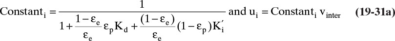
where ![]() and
and ![]() . The resulting velocities can be used in Eq. (19-29) and (19-30). The value of uport = L/tsw (derived in Problem 19.C10) is
. The resulting velocities can be used in Eq. (19-29) and (19-30). The value of uport = L/tsw (derived in Problem 19.C10) is
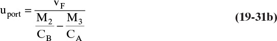
where CB is Constant from Eq. (19-31a) for solute with stronger adsorption (fructose).
C. Plan. We can calculate solute velocity constants Cgluc and Cfruc (fructose is more strongly adsorbed). Then uport can be found as a function of vF or F. Equations (19-29) and (19-30) can be used to calculate all other flow rates and L = uporttsw.
D. Do it. From Eq. (19-31a) for Constanti,
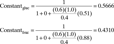
Feed velocity ![]() if F is in m3/min.
if F is in m3/min.
With Mi = 1.0, Eq. (19-31b) is
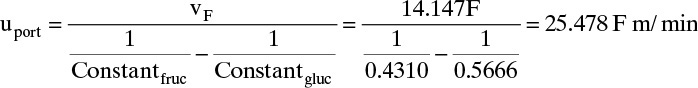
L = uporttsw = (25.478 F m/min) (5 min.) = 127.39 F (F in m3/min and L in m). From Eqs. (19-29b) and (19-15e) we obtain
v2 = M2 uport/Cfruc = (1.0)(25.478 F)/0.4310 = 59.113 F m/min
From Eq. (19-30b)
v3 = v2 – vF = 59.113 F – 14.147 F = 44.966 F
Similarly,
v1 = M1 uport/Cgluc = (1.0)(25.478 F)/0.5666 = 44.966 F = vrecycle
v4 = M4 uport/Cfruc = (1.0)(25.478 F)/0.4310 = 59.113 F
Then, from Eq. (19-30a), Eq. (19-30c), and Eq. (19-30d),
E. Check. As expected, D/F = 1.0, since all the Mi = 1.0. Also Aprod/F = vA, prod/vF = 1.0 and Bprod/F = 1.0.
F. Generalization. Equal values for feed, desorbent, and products; and v1 = v3, v2 = v4 occurs only for all Mi = 1. Usually, v4 is highest velocity and v1 is lowest. Further development of equations is done in Problem 19.C10. Note: From Eq. (19-31b) with uport > 0, there are limits to how small M2 and how large M3 can be. The form of the Constant in Eq. (19-31a) depends on the equation for solute velocity. For example, if equilibrium is q = Kx with q in g/g adsorbent and x in mass fraction, then the appropriate solute velocity equation is Eq. (19-15c) and the equation for the Constant is

To complete the design we need a value for F. Then velocities and pressure drops can be calculated (e.g., with Ergun equation). If pressure drop is too large, F or column diameter need to be adjusted. Because of dispersion and mass transfer resistances, products will not be 100% pure. Actual purities can be determined by experiment or detailed simulation (see Aspen Chromatography Lab AC7 in this chapter’s appendix). If more separation is needed, one can reduce M1 and M2 while increasing M3 and M4. TMBs (Figure 19-14A) are also of interest and can be analyzed with solute movement theory and by detailed simulations.
19.4 Nonlinear Solute Movement Analysis
Since most adsorption and ion exchange separations of commercial significance operate in the nonlinear region of isotherms, previous analyses need to be expanded to nonlinear systems. Nonlinear behavior is distinctly different from linear behavior, since one usually observes shock or constant pattern waves during feed steps and diffuse or proportional pattern waves during regeneration. Experimental evidence for constant pattern waves is shown in Figure 19-15A. The isotherm for carbon dioxide on activated carbon is a Langmuir-type shape. During loading we expect shock or constant pattern waves. This is clearly shown in the top figure, since waves can be moved along the time axis and easily be superimposed on each other. During desorption (elution) a diffuse or proportional pattern wave is expected (Figure 19-15B). These waves cannot be superimposed on each other. The width of proportional pattern waves is directly proportional to the distance waves travel in the column.
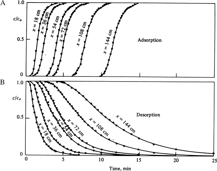
FIGURE 19-15. Adsorption and desorption of CO2 on activated carbon; (A) adsorption breakthrough curves illustrating constant pattern behavior, (B) desorption (elution) curves illustrating proportional pattern behavior, vsuper = 4.26 cm/s. Reprinted from Weyde and Wicke (1940).
Equations (19-14), which were derived for any type of isotherm, are starting points for analysis of solute movement with nonlinear isotherms. We need to substitute a specific nonlinear equilibrium expression to determine Δq/Δc. This insertion differs from inserting Δq/Δc = K′ for linear isotherms because the resulting expression is concentration dependent, and two separate forms result depending on initial column and feed concentrations. There are a huge number of expressions for nonlinear isotherms. To be specific, we focus on the Langmuir isotherm, Eqs. (19-5a), (19-6a), and (19-6c), which are popular forms.
19.4.1 Diffuse Waves
For an isotherm of Langmuir shape, if a column is initially loaded at some high concentration, chigh, and is fed with a fluid of low concentration, clow, a diffuse or proportional pattern wave results. Since derivative of q with respect to c exists,
We can now calculate this derivative for any desired nonlinear isotherm [for linear isotherms dq/dc = K′, and the result is Eq. (19-15)]. Specifically for Langmuir isotherm in Eq. (19-6c),
and solute wave velocity is
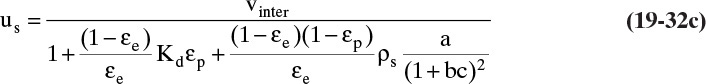
Note that for nonlinear isotherms solute wave velocity depends on concentration. For Langmuir isotherms, as solute concentration increases, the denominator in Eq. (19-32b) decreases and solute wave velocity increases. Another way to look at this is that dq/dc is the local slope or tangent of the isotherm. Figure 19-2 shows that for a Langmuir isotherm dq/dc is largest and thus velocity us is smallest as c approaches zero. Values for us can be calculated from Eq. (19-32c) for a number of specific concentrations, and the diffuse wave can be plotted as shown in Figure 19-16A. Times at which these solute waves, which are at known concentrations, exit column (at z = L) can be determined (see Figure 19-16A), and the outlet concentration profile can be plotted as in Figure 19-16B. Outlet wave varies continuously and is diffuse (not sharp). This result agrees with experiments that show zone spreading is proportional to column length and waves have a smooth, even spread in concentration. Analysis procedure is illustrated in Example 19-6.
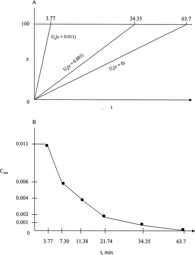
FIGURE 19-16. Diffuse wave analysis; (A) solute movement graph for Example 19-6, (B) predicted outlet concentration profile
A 100.0 cm long column is packed with activated alumina. Column is initially totally saturated at cA = 0.011 mol/L anthracene in cyclohexane solvent. It is then eluted with pure cyclohexane solvent (cA = 0) at a superficial velocity of 30.0 cm/min. Predict and plot outlet concentration profile using solute movement theory.
Data: εe = 0.42, εp = 0, Kd = 1.0, ρf (cyclohexane) = 0.78 kg/L, ρp = 1.465 kg/L, equilibrium ![]() where qA = mol anthracene/kg adsorbent and cA = mol anthracene/L solution.
where qA = mol anthracene/kg adsorbent and cA = mol anthracene/L solution.
Assume operation is isothermal.
Solution
A. Define. Find values of outlet concentration at different times using solute movement theory.
B. Explore. The most important decision is whether a diffuse or a shock wave (Section 19.4.2) will result. With a Langmuir isotherm a diffuse wave results when a more concentrated solution (cA = 0.011) is eluted with a dilute solution (cA = 0.0). If this is incorrect, the analysis will show us there is an error.
C. Plan. Since εp = 0, solute velocity (Eq. 19-32c) for a diffuse wave becomes
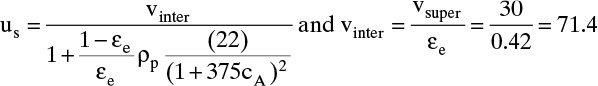
Substituting in parameter values, this becomes
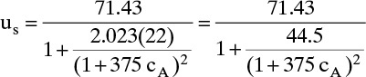
Since us depends on concentration, we can select arbitrary values of concentration ranging from cA = 0.011 to 0, calculate us, and determine tout = L/us.
D. Do it. Values are tabulated here for selected values of concentration.
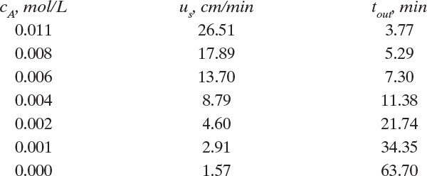
Solute movement solution using these values is shown in Figure 19-16A, and outlet concentration profile plotted from tabulated values of cA vs. tout is shown in Figure 19-16B.
E. Check. A check can be made with a mass balance over entire elution time.
–Outlet – Accumulation = 0
where the outlet concentration = ∫ Ac vsuper cA,out(t), and
accumulation = Ac ρs [qA(cA = 0) – qA(cA,F = 0.011)]
with qA determined from isotherm.
F. Generalize. The shape shown in Figure 19-16B, particularly strong tailing at very low concentrations, is typical of elution behavior with highly nonlinear isotherms. Complete removal of anthracene with an isothermal purge step will take a large amount of solvent.
Width of wave (in time units) at z = L is
Since width is proportional to column length L, this result agrees with experiments.
19.4.2 Shock Waves
For an isotherm with a Langmuir shape, if the column is initially loaded at some low concentration, cA,low, (cA,low = 0 if the column is clean) and is fed with a fluid of a higher concentration, chigh (see Figure 19-17A), a shock wave results. Feed steps in adsorption processes usually result in shock waves. Experiments show that when a shock wave is predicted, zone spreading is constant regardless of column length (a constant pattern wave). With the assumptions of solute movement theory (infinitely fast rates of mass transfer and no axial dispersion), the wave becomes infinitely sharp (a shock) and derivative dq/dc does not exist. Thus, the Δq/Δc term in denominator of Eq. (19-14) must be retained as discrete jumps in q and c, and shock wave velocity is
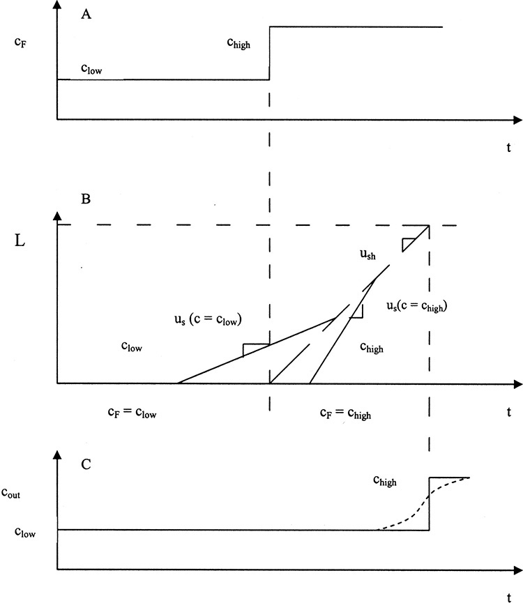
FIGURE 19-17. Shock wave analysis: (A) inlet concentration; (B) shock wave following Eq. (19-34); (C) outlet concentrations with solid line predicted by solute movement theory, and dashed line representing experimental result (modified from Wankat, 1986). Reprinted with permission, copyright, 1986 Phillip C. Wankat.
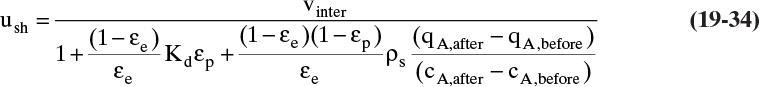
where subscripts “before” and “after” refer to conditions immediately before and immediately after the shock wave. Fluid and solid before the shock wave (cA,before and qA,before) are assumed to be in equilibrium, as are values of cA,after and qA,after after the shock wave. For a general Langmuir isotherm, Eq. (19-6c), shock wave velocity is
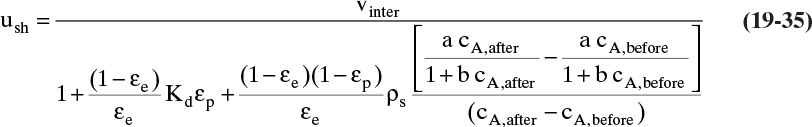
Shock wave velocity depends on concentrations on both sides of the shock wave. The resulting shock wave is shown in Figure 19-17B, and outlet concentration is shown in Figure 19-17C. Superficially, the outlet concentration profile in Figure 19-17C looks like results from a linear isotherm (concentration jumps to cfeed). However, for linear isotherms this outlet step occurs at t = L/us, which is constant regardless of feed and initial concentrations. The shock wave outlet step occurs at t = L/ush, which depends on both feed and initial concentrations. In addition, shock waves are self-sharpening, a concept explored in Example 19-7. Waves in systems with linear isotherms are not self-sharpening.
EXAMPLE 19-7. Self-sharpening shock wave
A 100.0 cm long column is packed with activated alumina. The column is initially filled with pure cyclohexane solvent (cA = 0.0 mol/L anthracene). At tF1 = 0, feed 1 containing cA,F1 = 0.0090 mol/L anthracene in cyclohexane solvent is input. At tF2 = 10 minutes, feed 2 containing cA,F2 = 0.011 mol/L anthracene in cyclohexane solvent is input. Superficial velocity is 20.0 cm/min. Predict and plot outlet concentration profile using solute movement theory.
Data: εe = 0.42, εp = 0, Kd = 1.0, ρf (cyclohexane) = 0.78 kg/L, ρp = 1.465 kg/L, equilibrium: qA = 22cA/(1 + 375cA) where qA = mol anthracene/kg adsorbent and cA = mol anthracene/L solution.
Solution
A. Define. Find outlet concentration at different times using solute movement theory.
B. Explore. The most important decision is whether a diffuse or a shock wave (Section 19.4.2) will result for each feed step. With a Langmuir isotherm a shock wave results when a concentrated feed is fed to a column that is initially more dilute. For example, cA,F1 = 0.009 fed to column with cA,1,initial = 0.0, and also cA,F2 = 0.011 fed to column with cA,2,initial = 0.009. Thus we expect a first shock wave followed after 10 minutes by a second that, as we will see, is faster. If they intersect, there will be a third shock wave (feed cA,F2 = 0.011 and cA,initial = 0.0). Realizing that there could be a third shock wave (see Figure 19-18A) is probably the hardest part of this problem.
FIGURE 19-18. Analysis and results for Example 19-7: (A) solute movement diagram showing intersection of two shock waves, (B) outlet concentration profile
C. Plan. Shock velocity can be calculated from Eq. (19-35) with εp = 0. With εp = 0, solid density ρs is equal to particle density ρp. Interstitial velocity is
vinter = vsuper/εe = 20.0/0.42 = 47.62 cm/min
Substituting in values of parameters, except for ΔqA/ΔcA, the shock wave velocity is
where
For shock wave 1, cA,initial = 0, qA (cA,initial) = 0, and cA,F1 = 0.009. qA,sh1 (cA,F1) is calculated from Langmuir isotherm followed by calculation of ΔqA/ΔcA and uA,sh1. A similar calculation can be done to calculate uA,sh2. Then we calculate the time and distance the two shock waves intersect. If intersection occurs at z < 100 cm, there is a third shock wave.
D. Do it. Shock wave 1 (cA,initial,1 = 0, cA,F1 = 0.009):
Shock wave 2 (cA,initial,2 = 0.009, cA,F2 = 0.011), and qA,initial,2 = 0.04526. Calculate qA(cA,F2) from Langmuir isotherm, ![]() , and velocity of shock wave from Eq. (19-34),
, and velocity of shock wave from Eq. (19-34), 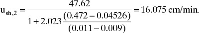
The solute movement diagram is shown in Figure 19-18A. The intersection of the two shock waves occurs at zintersect, tintersect. We can calculate the point of intersection of the two waves by noting that the first shock wave travels zintersect = ush,1 tintersect, and the second shock wave travels zintersect = ush,2 (tintersect – 10). Setting these equal and solving for tintersect,
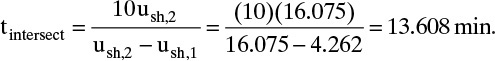
Then zintersect = (4.262cm/min)(13.608 min) = 58.0 cm.
After this distance, there is a third shock wave with cA,initial,3 = 0.0 (the initial column concentration at t = 0) and cA,F2 = 0.011 (feed concentration after 10 minutes). Since qbefore and qafterwere previously calculated, ush,3 can be determined.
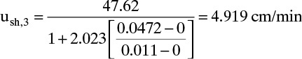
This shock exits at ![]()
The complete solute movement diagram is shown in Figure 19-18A, and outlet concentration profile is shown in Figure 19-18B.
E. Check. As expected, ush,2 > ush,3 > ush,1. We can check mole balance from t = 0 to t = 22.146 minutes. Because concentration is zero until breakthrough occurs, there is no outlet of anthracene:
Inlet anthracene from t = 0 to t = 22.146 minutes = Accumulation anthracene
Inlet consists of feed 1 (cA,F1 = 0.009 mol/L) from tF1 = 0 to tF2 =10 minutes and feed 2 (cA,F2 = 0.011) until breakthrough at tbreakthrough = 22.146 minutes. Thus
Inlet = vsuperAc[cA,F1 (tF2 – tF1) + cA,F2 (tbreakthrough – tF2)]
Accumulation is final condition [adsorption at qA(cA,F2 = 0.011) = 0.0472 plus fluid in pores at cA,F2 = 0.011] minus initial condition [cA,initial = 0 and qA,initial = 0]. This mole balance is satisfied (see Problem 19.D32).
F. Generalize. A single shock wave results when two steps are input because of self-sharpening behavior of shock waves. Diffuse waves can also be sharpened if they are followed with a shock wave. This phenomenon is used in commercial cycles. Regeneration requires less purge if an adsorbate tail (called a heel) is left in the column (see Figure 19-16B). This diffuse wave is then sharpened when the next feed step forms a shock wave.
In experiments (Figure 19-15A) outlet concentration profiles are not sharp, as shown in Figures 19-17B and 19-18B. Instead, finite mass transfer rates and finite amounts of axial dispersion spread waves, while the isotherm effect (illustrated in Example 19-7) counteracts this spreading. The final result is a dynamic equilibrium where waves spread a certain amount and then stop spreading. Once formed, this constant pattern wave has a constant width regardless of column length.
Interaction of shock and diffuse waves can be analyzed with the theory presented in this section (see Problem 19.E1). If there are two or more adsorbates that compete for sites [e.g., with multicomponent Langmuir isotherms, Eq. (19-8)], interactions often occur between shock waves and diffuse waves from different components (e.g., Ruthven, 1984; Yang, 1987). Theories for two or more interacting solutes are beyond the scope of this introductory chapter.
19.5 Ion Exchange
Ion exchange is a unit operation in which ions held on a solid resin are exchanged for ions in feed solution. For most people water softening is the only familiar ion exchange system. In water softening calcium and magnesium ions (“hard” water ions) in the feed are replaced with sodium ions (“soft” water ions). If feed containing calcium and magnesium is continued, eventually resin will become saturated with these ions and no additional exchange occurs. To produce soft water, resin needs to be regenerated, which can be done with a concentrated solution of sodium chloride salt. A number of other ion exchange separations are done commercially.
The most common materials used for ion exchange are polymer resins with charged groups attached (Anderson, 1979; Dechow, 1989; LeVan et al., 1997; Wankat, 1990). Cation exchange resins have fixed negative charges, whereas anion exchange resins have fixed positive charges. Resin is called strong if it is fully ionized and weak if it is not fully ionized. Most commonly used strong resins are based on polystyrene (see Figure 18-3E) cross-linked with divinylbenzene (DVB) with benzene-sulfonic acid groups attached to polystyrene. Most common strong anion exchange resins have a quaternary ammonium structure. Cross-linked polystyrene resins are commonly used for water treatment and have very good chemical resistance, although they are attacked by chlorine. Copolymers of DVB and acrylic or methacrylic acid are used for weak acid resins. No single type of weak base resin is dominant, although use of a tertiary amine group on a polystyrene-DVB resin is common. Although capacity of weak exchangers is lower than for strong resins, they also require less regenerant. Weak resins tend to be less robust than strong resins and need to be protected from chemical attack. Table 19-4 lists typical properties of ion exchange resins.
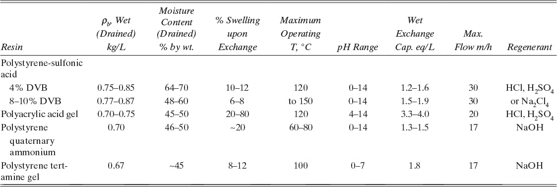
TABLE 19-4. Properties of common ion exchange resins (LeVan et al., 1997; Wankat, 1990)
Ion exchange involves a reversible reaction between ions in solution and ions held on resin. An example of monovalent cation exchange is removal of sodium ions from resin using hydrochloric acid:
In this equation R– represents fixed negative charges such as SO3– on resin. Hydrogen and sodium ions that are exchanging are called counter-ions. Chloride ion, which has same charge as the fixed SO3– groups, is called the co-ion. Although chloride ion does not directly affect reaction, at high concentrations it does affect equilibrium. Exchange of a divalent cation with a monovalent cation is also common and is exemplified by removal of calcium ions from water and replacement with sodium ions (water softening).
where X– is any anion. Of course, there are a variety of other possibilities.
Standard practice is to define equivalent fractions of ions in solution, xi, and on resin, yi,
where ci is concentration of ion i in solution (e.g., in equivalents/m3), cT is total concentration of cations or anions in solution, cRi is concentration of ion i on resin (in volume units such as equivalents/m3), and cRT is total concentration of ions on resin. Total concentration of ions on resin cRT, the resin capacity, is a constant equal to concentration of fixed negative sites set when resin is made. One advantage of using equivalent fractions is that they must sum to one.
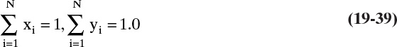
19.5.1 Ion Exchange Equilibrium
For a simplified view of ion exchange equilibrium for binary ion exchange, assume the equilibrium constant can be determined by the law of mass action. Let A represent hydrogen ions and B sodium ions. For monovalent ion exchange,
A+ + RB + X– = AR + B+ + X–
Illustrated in Eq. (19-36), the mass action equilibrium expression simplifies to

where local concentrations of co-ion X– in the resin interior are identical (and very low) in numerator and denominator and hence cancel. (These concentrations are very low in resin because of a phenomenon known as Donnan exclusion—the very high concentrations of fixed charges on resin exclude free anion X– from the resin.) Equilibrium constant KAB isn’t really constant (e.g., see Wankat, 1990), but in dilute solutions it will be close to constant. Solving Eq. (19-40a) for yA,

The order of subscripts is important, KBA = 1/KAB. These equations can be applied to any monovalent exchange by substituting in appropriate symbols for exchanging ions. Experimental values for equilibrium constants are required. A few representative values are given in Table 19-5. If we know equilibrium constants KAB and KCB, we can calculate value of KCA from
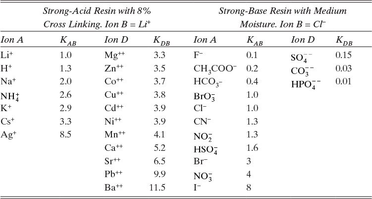
TABLE 19-5. Approximate equilibrium constants for ion exchange (Anderson, 1997)
This result expands the usefulness of Table 19-5. However, since values in Table 19-5 are approximate (e.g., Dechow [1989] lists the following values for strong acid resins: H+ = 1.26, Na+ = 1.88, ![]() , K+ = 2.63, Cs+ = 2.91, and Ag+ = 7.36), they should not be used for detailed design calculations.
, K+ = 2.63, Cs+ = 2.91, and Ag+ = 7.36), they should not be used for detailed design calculations.
The equilibrium expression for a divalent ion exchanging with a monovalent ion [e.g., reaction in Eq. (19-37)] is not as simple. If D represents divalent calcium ion and B monovalent sodium ion, reaction is
D+2 + RB2 + 2X– = RD + 2B+ + 2 X–
and equilibrium constant from the mass action expression is
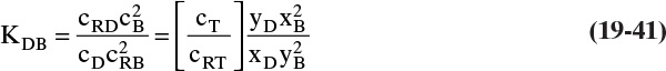
Selected values of divalent-monovalent equilibrium constants are given in Table 19-5. If KDB and KAB are known, then the desired constant KDA is
Substituting summation Eqs. (19-39) into Eq. (19-41), we obtain the equilibrium expression,
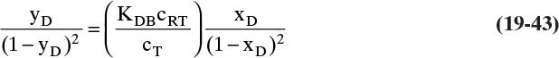
This equation can conveniently be solved for yD for any specified value of xD using the formula for solution of quadratic equations or by using Goal Seek or Solver in a spreadsheet. Note that the effective equilibrium parameter in Eq. (19-43) is (KDB cRT /cT). Since total concentration in fluid can easily be changed, this effective equilibrium parameter can be changed. This behavior can be useful in water softening and is illustrated in Example 19-8 and Figure 19-19.
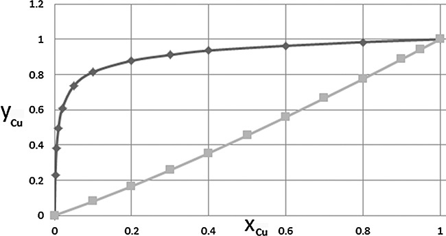
FIGURE 19-19. Equilibrium for copper-sodium exchange for Example 19-8; ![]() cT = 0.01 N,
cT = 0.01 N, ![]() cT =2.5 N
cT =2.5 N
Equilibrium parameters are temperature dependent. However, ion exchange is usually operated at a constant temperature near ambient.
19.5.2 Movement of Ions
Solute movement theory developed in Sections 19.3. and 19.4. can be extended to ion movement. For gel-type ion exchange resins, which are most popular, there are no permanent pores, and εp = 0. Development of solute movement theory is modified by setting εp = 0, expressing concentrations in terms of equivalent fractions x and y, and including a Donnan exclusion factor KDE. The result is
Co-ions (ions with the same charge as ions fixed to resin) are excluded, and they have KDE = 0. Exchanging ions are not excluded, and KDE = 1. Note that (1 –εe) ρs does not appear in Eq. (19-44) because volumetric units are commonly used for ion concentrations in solution and on resin.
Equation (19-44) can be applied to either diffuse or shock waves. Diffuse waves occur if a column that is concentrated in ion A (or D) is fed a solution of low concentration A (or D) and KAB > 1.0 [or (KDB cRT /cT) > 1.0]. If KAB < 1.0 [or (KDB cRT /cT) < 1.0] diffuse waves occur when a column that has a dilute amount of ion A (or D) is fed a solution that is concentrated in A (or D). For diffuse waves ion velocity is
The derivative (dyi/dxi) can be determined from the appropriate equilibrium expression, such as Eq. (19-40b) or Eq. (19-42b). These derivatives are

for monovalent-monovalent exchange and
for divalent-monovalent exchange.
Shock waves occur when conditions are opposite of those for diffuse waves. For example, if KAB > 1.0 [or (KDB cRT /cT) > 1.0] and a solution concentrated in A (or D) is fed to a column containing a dilute solution of ion, a shock wave would be expected. The shock wave equation is
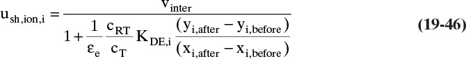
Equivalent concentrations of ion A (or D) in solution xi and on resin yi are assumed to be in equilibrium both before and after the shock wave.
Note that ion velocities depend on the ratio (cRT/cT) regardless of the isotherm form. This agrees with our physical intuition. If resin capacity cRT is high while concentration of ion in solution cT is low, we would expect that waves would move slowly.
Because changes in the total ion concentration can affect both equilibrium and ion velocities, we need to balance total ion concentration. When feed total ion concentration is changed, an ion wave passes through the column. For relatively dilute solutions resin is already saturated with counter-ions, and more ions cannot be retained. For a total ion balance, total ions are excluded, KDE = 0, and Eq. (19-44) becomes
The same result is obtained for co-ions. Total ion and co-ion waves move rapidly through the column. A total ion wave affects counter-ion (uA or uD) velocities for all ion exchange systems.
For exchange of ions of equal charges (e.g., monovalent-monovalent), equilibrium is not affected by a total ion wave and xi,after = xi,before and yi,after = yi,before. Equilibrium for exchange of ions with different charges (e.g., divalent-monovalent or trivalent-monovalent) is changed. A mass balance on a segment of column (see Problem 19.C9) shows that
For monovalent-monovalent exchange,
while for divalent-monovalent exchange,
but xafter_total_ion_wave is in equilibrium with yafter_total_ion_wave.
The calculation of these effects is illustrated in Example 19-8.
EXAMPLE 19-8. Ion movement for divalent-monovalent exchange
A 50 cm long ion exchange column is filled with a strong acid resin (cRT = 2.0 equivalents/L, εe = 0.40). The column initially is at a total cation concentration of cT = 0.01N with xNa = 0.90, xCu = 0.10. Chloride is co-ion. At t = 0, we feed a 2.5 N aqueous solution of NaCl (xNa = 1.0). Selectivity constants can be calculated from Table 19-5. Counter-ions are not excluded (KE = 1.0). Superficial velocity throughout the experiment is 20.0 cm/min.
Predict
A. Equilibrium behavior at cT = 0.01 N and at cT = 2.5 N.
B. Time total ion wave exits.
C. Values of xCu and yCu after total ion wave exits.
D. Time and shape of exiting sodium wave.
Solution
A. Define. First, find equilibrium parameters at cT = 0.01 N and at cT = 2.5 N and plot equilibrium results. Then, find breakthrough time for total ion wave, equivalent fractions of copper at cT = 2.5 N, and outlet concentration profile for sodium.
B. Explore. Determination of equilibrium behavior, ion wave, and values of xCu and yCu follows the equations, but the order can be a bit confusing. One reason for showing this example is to clarify how the calculations proceed. Sometimes, the biggest challenge is determining if the sodium wave is a shock or diffuse wave.
C. Plan. Selectivity can be found from Eq. (19-42), and equilibrium parameter is (KDB cRT/cT). Equilibrium curves can be found at arbitrary x values from Eq. (19-43). Velocity of total ion wave is equal to interstitial velocity. Equivalent fractions of copper can be found by solving Eq. (19-43) with xCu,before = 0.10 and cT,before = 0.01 N to find yCu,before. After total ion wave passes, solve Eq. (19-43) for xCu,after with yCu,after = yCu,before and cT,after = 2.50 N. Finally, sodium breakthrough time can be calculated from either Eq. (19-45) or Eq. (19-46) after we decide if it is a diffuse or shock wave, respectively. To determine the nature of the sodium wave, we will look at the isotherm shape and type of wave that occurs for a decrease in copper concentration in the feed.
D. Do it. First, find the equilibrium curve at cT = 0.01 N. Since copper is divalent and sodium is monovalent, use Eqs. (19-42) and (19-43). From Eq. (19-42)

Then Eq. (19-43) becomes 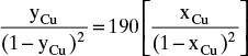 .
.
At xCu= 0.1 (initial concentration), 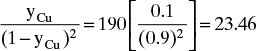 .
.
Solving for yCu with a spreadsheet, we obtain yCu = 0.814. The following equilibrium table at cT = 0.01 N was generated using this spreadsheet.

When cT = 2.5 N, ![]() and Eq. (19-43) is
and Eq. (19-43) is ![]() . Equilibrium results at cT = 2.5 N are
. Equilibrium results at cT = 2.5 N are

The two equilibrium tables are plotted in Figure 19-19. Note that with cT = 0.01 N a very favorable isotherm results, but with cT =2.5 N the isotherm is unfavorable.
Velocity of the total ion wave is utotal_ion = vsuper/εe = vinter = 20.0/0.4 = 50 cm/min, and breakthrough time of this wave is tbr = L/utotal_ion = 50.0/50.0 = 1.0 min.
From the table of equilibrium values at cT = 0.01 N, when xCu,before = 0.10, yCu,before = 0.814. Then, after total ion wave passes and cT = 2.5 N, yCu,after = yCu,before = 0.814. At cT =2.5 N and yCu,after = 0.814, we can solve Eq. (19-41c) for xCu,after.
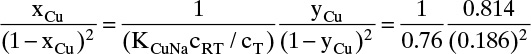
The result is xCu,after = 0.836. The large increase in copper equivalent fraction in liquid is caused by change in equilibrium at higher total ion concentration. Increase in copper is supplied by removing copper from resin when the total ion wave passes.
The 2.5 N sodium chloride regeneration solution contains no copper, xCu,2.5N solution = 0, which causes a sodium wave to pass through the column. Since the column is at 2.5 N when a sodium wave reaches any part of the column, we use that equilibrium curve in Figure 19-19. This is an unfavorable isotherm for copper; thus, with a drop in copper concentration in the feed, a shock wave results, and Eq. (19-46) with KDE = 1 is used to calculate shock wave velocity.
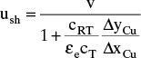 where ΔyCu = yCu,after Nacl – yCu, before Nacl = 0.0 – 0.814 = –0.814
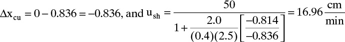
This shock wave exits at tNaCl = L/ush = 50/16.96 = 2.95 minutes. The solute movement diagram is plotted in Figure 19-20.
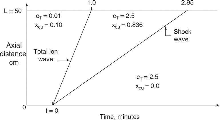
FIGURE 19-20. Solute movement diagram for Example 19-8
E. Check. A copper mass balance on the entire cycle can be used as a check:
Cu in – Cu out = Cu accumulation
From t = 0 to t = 2.95 minutes, there is no copper flowing into the system. The outlet copper amount consists of 1 minute at (cT = 0.01 N, xCu = 0.10) and 1.95 minutes at (cT = 2.5 N, xCu = 0.836), as shown in Figure 19-20. Since we know the conditions at the beginning of the cycle (cT = 0.01 N, xCu,before = 0.10, yCu,before = 0.814) and at the end of the cycle (cT =2.5 N, xCu,after_NaCl = 0.0, yCu,after_NaCl = 0.0), we can calculate the accumulation term for the cycle. The mass balance then becomes
0 – (vsuper = 20)Ac[(1.0 min)(cT = 0.01)(xcu = 0.10) + 1.95 min (cT = 2.5)(xcu = 0.836)]
= –Ac(L = 50)(cRT = 2.0)[(ycu = 0.814) – (ycu = 0)]
or –81.5 Ac = –81.4 Ac
This is certainly within the accuracy of the calculations.
F. Generalization. The change in equilibrium behavior from a favorable isotherm to an unfavorable isotherm when cT is increased occurs only for exchange of ions with unequal charges. This change can result in shock waves during both the feed and regeneration steps. Since shock waves show significantly less spreading than diffuse waves, significantly less regenerant is required. This phenomenon is used to advantage in water softeners that exchange “hard” Ca++ and Mg++ ions (they precipitate when heated and foul cooking utensils or heat exchangers and interfere with soap) at very low cT values with Na+ ions. Regeneration is done with a concentrated salt (NaCl) solution at high cT.
This introductory presentation on ion exchange has been restricted to dilute solutions with exchange of two ions. A variety of more complex situations, including complex equilibria and mass transfer, partial ion exclusion, resin swelling (see Table 19-4), and backwashing to remove dirt, often occur in practice but are beyond the scope of this introductory section. Information about a variety of phenomena, different equipment, equilibrium theory, and mass transfer are discussed by Helfferich (1962) and Dechow (1989).
19.6 Mass and Energy Transfer in Packed Beds
For detailed predictions and understanding of sorption separations, we need to do a detailed analysis of diffusion rates, mass and energy transfer, and mass and energy balances in the column. In order to make results somewhat tractable, we will make the usual assumptions listed in Table 19-6.
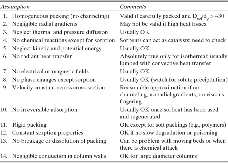
Fluid flowing in external void volume in Figure 19-1 is usually assumed to have a constant concentration (or partial pressure) at each axial distance z; thus this bulk concentration is not a function of radial distance from the center of the bed. During the course of separation, sorbates are first transferred down the column by bulk transfer. Sorbates then transfer across the external film and diffuse in pores until they reach sorbent sites. At these sites they are sorbed in a usually rapid step. For an equilibrium system, some sorbates will always be desorbing and diffusing back into bulk fluid. Desorption is favored during regeneration by increasing temperature or dropping sorbate concentration.
Since the first step in separation, bulk transport, is assumed to be rapid enough to keep bulk concentration (at any given value of z, t) constant, we start with an analysis of film mass transfer.
19.6.1 Mass Transfer and Diffusion
Mass transfer across the film (see Figure 19-1) occurs by a combination of diffusion and convection. As is usual in film mass transfer, driving force is assumed to be (c – cpore) where the concentration in pores cpore is calculated at the particle surface. The film transfer term becomes –kf ap (c – cpore) where kf is film mass transfer coefficient (m/s) and ap is surface area of particles per volume (m–1). For spherical particles
With porous particles the film equation is a bit more complicated than in Chapter 15, since accumulation of mass in particles is distributed between pores and solid. The resulting equation is

The left-hand side of this equation is accumulation of solute on solid and in fluid within the pores. The right-hand side is mass transfer rate across the film. Since amount adsorbed in particles and concentration of pore fluid are functions of r, terms ![]() and
and ![]() are defined as average amount adsorbed in particle and average pore fluid concentration, respectively.
are defined as average amount adsorbed in particle and average pore fluid concentration, respectively.
A more familiar looking version of the film transport equation is obtained for a single-porosity model. This result can be formally obtained by setting εp = 0 and εe = ε in Eq. (19-48b).

Since film mass transfer rates are usually quite high compared to diffusion in the particles, film resistance is rarely important in commercial processes (Basmadjian, 1997).
After passing through the film, solute diffuses in pores by normal diffusion (normal pores), Knudsen diffusion (small pores), or surface diffusion. In polymer resins where there are no permanent pores, solute diffuses in the polymer phase. For spherical particles with a radial coordinate r, the diffusion equation in pores is

For ordinary or Fickian diffusion Deffective is related to diffusivity in free solution through the tortuosity factor, Eq. (19-4). Equation (19-50) assumes the mean free paths of molecules are significantly less than the radius of the pores. This is the usual case with liquids and with gases at high pressures.
Knudsen diffusion occurs when the mean free paths of molecules are significantly greater than the pore radius. In this case instead of colliding with other molecules, a molecule collides with pore walls. The same diffusion equation can be used, but now Deffective is determined from Eq. (19-4) with DK, Knudsen diffusivity replacing Dmolecular. Knudsen diffusivity can be estimated from (Yang, 1987)
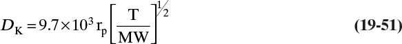
where pore radius rp is in cm, absolute temperature T is in Kelvin, MW is molecular weight of solute, and DK is in cm2/s. If the mean free path of molecules is the same order of magnitude as pore diameter, both ordinary and Knudsen diffusion mechanisms are important. Diffusivity can be estimated as
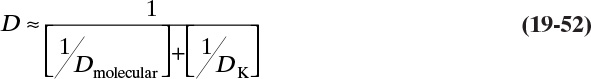
This value of D is then used instead of Dmolecular in Eq. (19-4) to estimate Deffective. Use of Eqs. (19-51) and (19-52) is often required for adsorption of gases in adsorbents with small pores.
In surface diffusion adsorbate does not desorb from the surface but instead diffuses along the surface. This mechanism can be important in gas systems and when gel-type (nonporous) resins are used. Surface diffusion flux is

where surface diffusion coefficient Ds depends strongly on surface coverage, q. Currently, values of Ds must be back-calculated from diffusion or adsorption experiments. Ordinary, Knudsen, and surface diffusion may occur simultaneously. More detailed descriptions of diffusion terms are available in books by Do (1998), Ruthven (1984), and Yang (2003).
19.6.2 Column Mass Balances
Equations for film diffusion and diffusion inside particles tell us what is happening at a given column location. To determine what is happening for the entire column we need a mass balance on solid and fluid phases. In order to write reasonably simple balance equations, we usually make a number of “common-sense” assumptions such as those listed in Table 19-6. The resulting equation for a two-porosity model is

The first three terms are accumulation in fluid between particles, within pore fluid with an average concentration ![]() and sorbed on solid, respectively. The fourth term represents convection, and the fifth term is axial dispersion. Coefficient ED is axial dispersion coefficient due to both eddy and molecular effects.
and sorbed on solid, respectively. The fourth term represents convection, and the fifth term is axial dispersion. Coefficient ED is axial dispersion coefficient due to both eddy and molecular effects. ![]() can be related to ci and
can be related to ci and ![]() through Eqs. (19-48b) and (19-50). A slightly simpler equation is obtained with a single-porosity model:
through Eqs. (19-48b) and (19-50). A slightly simpler equation is obtained with a single-porosity model:

Solution of an appropriate set of equations—equilibrium, Eqs. (19-48b) or (19-49), diffusion Eq. (19-50) [with diffusivities calculated from Dmolecular, Eq. (19-51), or (19-52) inserted into Eq. (19-4) and/or use of Eq. (19-53)], and with column mass balance Eq. (19-54) or (19-55) plus a suitable set of boundary conditions—is very difficult. This calculation is so difficult that even with detailed simulators a simplified procedure is often employed.
19.6.3 Lumped Parameter Mass Transfer
One very common simplification is to assume that film diffusion and diffusion in particles can be lumped together in a lumped parameter mass transfer expression. In this form the mass transfer rate is assumed to be proportional to a driving force caused by concentration difference ![]() or by difference in amount adsorbed
or by difference in amount adsorbed ![]() is concentration that would be in equilibrium with
is concentration that would be in equilibrium with ![]() , and
, and ![]() is amount adsorbed that would be in equilibrium with fluid of concentration ci. Note that neither
is amount adsorbed that would be in equilibrium with fluid of concentration ci. Note that neither ![]() nor
nor ![]() actually exist in the column—they are hypothetical constructs. The two resulting equations are
actually exist in the column—they are hypothetical constructs. The two resulting equations are


Equation (19-56a) is very similar to Eq. (19-48b) except that c* replaces concentration of pore fluid cpore and lumped parameter mass transfer coefficient km,c replaces film coefficient kf. As expected, lumped parameter expressions using a single-porosity model are simpler:


Equations (19-56a) and (19-56b) or (19-57a) and (19-57b) can be converted into each other if equilibrium is linear (km,q = km,c/K′). Since both Eqs. (19-57a) and (19-57b) are commonly used, it is necessary to be clear which lumped parameter coefficient is reported—unfortunately, authors usually don’t put a subscript denoting driving force on k. Look for their driving force equation to determine which form they used.
Although they produce approximations, lumped parameter models are useful because they simplify theory and coefficients can often be estimated with reasonable accuracy. km,q is commonly determined with a sum of resistances approach (Ruthven et al., 1994) that is similar to the approach used in Section 15.1.

Mass transfer area per volume, ap, is usually estimated as 6/dp. A number of correlations have been developed to estimate film coefficient. The Wakao and Funazkri (1978) correlation appears to be quite accurate:
where the Sherwood, Schmidt, and Reynolds numbers are defined as

A final value needed to solve the complete set of equations is eddy dispersion coefficient, ED. The Chung and Wen (1968) correlation is commonly used to determine ED:
where the Reynolds number was defined in Eq. (19-60) and the Peclet number is defined as
In many systems, particularly liquid systems, resistance due to pore diffusion is much more important than resistance due to film mass transfer [Deffective is small and hence the second term on the right-hand side of Eq. (19-58a) is much larger than the first term]. Then,

Thus, when pore diffusion controls, the mass transfer coefficient is independent of fluid velocity and proportional to (1/dp)2. Basmadjian (1997) suggests that initial estimates can be made with km,cap values of 10–1 1/s for gases and 10–2 to 10–3 1/s for liquids. More detailed discussions of kinetics and mass transfer in adsorbents can be found in books by Do (1998), Ruthven (1984), and Yang (2003).
19.6.4 Energy Balances and Heat Transfer
Since there are often significant heat effects in gas systems, energy balances will be required. For a single-porosity model the energy balance (based on assumptions in Table 19-6) for fluid, particles, and column wall is

The first two terms and last term represent accumulation of energy in fluid, particle, and column wall. The third term is convection of energy, and the fourth term is axial dispersion of energy. The fifth term (first term on right-hand side) represents heat transfer from column walls. Because industrial-scale systems have a small ratio of wall area to column volume, the fifth term is often negligible (column is adiabatic), and the sixth term is often negligible because mass of column wall is small compared to mass of adsorbent.
Transfer of energy from fluid to solid can often be represented as a lumped parameter expression:

The first term is accumulation of energy in solid, the second term is heat transfer rate from fluid to solid, and the last term is heat generated by adsorption. This last term can be quite large. Increases in gas temperature of over 100°C can occur in gas adsorption systems, and if oxygen is present, activated carbon beds can catch fire.
19.6.5 Derivation of Solute Movement Theory
The solute movement equations can be derived rigorously by solving mass and heat transfer equations with a set of limiting assumptions. Start with a column balance on fluid and solid, Eq. (19-54). Assuming that mass transfer is very rapid, bulk fluid and solid will be in equilibrium. Thus c = c*, which is in equilibrium with q = q*, and lumped parameter expression, Eq. (19-56a) or (19-56b), is not required. In addition, assuming axial dispersion is negligible, Eq. (19-54) becomes

Since solid and fluid are in equilibrium, q is related to c and T through the isotherm. After assuming solid properties (εe, εp, Kd, and ρs) are constant, applying chain rule and simplifying, Eq. (19-65a) becomes

The total derivative dT/dt = 0 for isothermal systems, systems with instantaneous temperature changes, and systems with square wave changes in the temperature. With these simplifications Eq. (19-65b) can be solved by the method of characteristics (e.g., Ruthven, 1984; Sherwood et al., 1975). The result for constant interstitial velocity (valid for liquids, exchange adsorption, and dilute gases) is that concentration is constant along lines of constant solute velocity where the solute velocity is given by Eq. (19-14).
A similar analysis can be applied to the energy balance equation by assuming very rapid energy transfer, negligible axial thermal diffusion, constant solid and fluid properties (e.g., densities and heat capacities), constant interstitial velocity, and negligible heat of adsorption. The result is that temperature is constant along lines of constant thermal velocity where thermal velocity is given by Eq. (19-21).
Solute movement analysis is thus a physically based analysis that can be derived rigorously with appropriate limiting assumptions. If mass transfer is slow and velocity is high or the column is short, solute may not have sufficient residence time to diffuse into solid. Solute then skips the separation mechanism (equilibrium between solid and fluid) and exits with the fluid void volume. In this situation predictions of solute movement are not useful. Basmadjian (1997) states that one of the following conditions must be satisfied to avoid bypassing or “instantaneous breakthrough”:
Local equilibrium analysis can be extended to systems with variable interstitial velocity (concentrated gases), interacting solute isotherms such as Eq. (19-8), or finite heats of adsorption (concentrated gases), but these extensions are beyond this chapter’s scope (e.g., see Ruthven, 1984; Yang, 1987).
19.6.6 Detailed Simulators
Simultaneous solution of combined mass and energy balances, pressure drop equation [see Eq. (19-90)], and equilibrium expressions is a formidable task, particularly for multicomponent, nonlinear systems. Until the 1990s, solution of this set of differential, algebraic equations (DAE) was typically a task done by Ph.D. students for their thesis or by a few industrial experts who devoted their careers to simulation of sorption processes. This situation changed with development of fairly general solvers for DAEs, such as SPEEDUP, gPROMS, and Aspen Custom Modeler, and later development of simulators such as ADSIM and Aspen Chromatography designed specifically for adsorption, chromatography, and ion exchange. Current versions of DAE solvers and simulators are reasonably user friendly. Currently, almost all distillation and absorption processes are designed using simulators. In the future most designs of sorption systems will be based on simulation programs. Teaching use of these simulation packages is discussed by Wankat (2006), and computer laboratories for Aspen Chromatography are included in this chapter’s appendix.
In the next two sections mass and energy transfer equations are used to obtain realistic solutions for a variety of simplified adsorption problems.
19.7 Mass Transfer Solutions for Linear Systems
Solution of differential equations is much simpler when equations are linear. The various sets of differential equations for mass transfer discussed in Section 16.6 are all linear if equilibrium isotherm is linear and operation is isothermal. [Nonisothermal operation introduces Arrhenius relationship, Eq. (19-7), which is decidedly nonlinear.] This section is limited to isothermal operation of systems with linear isotherms.
The zone spreading observed in solutions of Eqs. (19-54) and (19-55) for linear isotherms looks identical regardless of whether it is caused by mass transfer resistances, axial dispersion, or both. Thus, from an experimental result it is impossible to determine if spreading was caused solely by mass transfer resistances, solely by axial dispersion, or by a combination of both. This property of linear systems allows us to use simple models to predict behavior of more complex systems.
19.7.1 Lapidus and Amundson Solution for Local Equilibrium with Dispersion
In a classic paper Lapidus and Amundson (1952) studied liquid chromatography for isothermal operation with linear, independent isotherms when mass transfer is very rapid, but axial dispersion is important. Although a two-porosity model can be used (Wankat, 1990), solution was originally obtained for a single-porosity model. Starting with Eq. (19-55), substitute in equilibrium expression Eq. (19-6a) to remove variable q (solid and fluid are assumed to be in local equilibrium). Since fluid density is essentially constant in liquid systems, interstitial fluid velocity vinter is constant. The resulting equation for each solute is

For a step input from c=0 to c=cF, the boundary conditions used by Lapidus and Amundson were
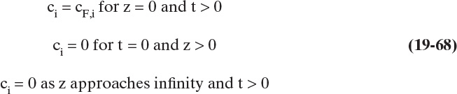
The last boundary condition, the infinite column boundary condition, greatly simplifies solution. It is approximately valid for long columns.
For sufficiently long columns, solution for each solute is
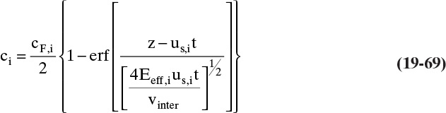
where us,i is the single-porosity form of the solute velocity, Eq. (19-15b) (included in Problem 19.C5). The term erf is the error function, which is definite integral:
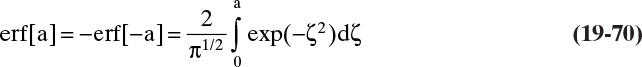
Since the error function is a definite integral, for any value of argument (value within brackets) the error function is a number. Error function values can be calculated from the normal curve of error available in most handbooks, are tabulated in Wankat (1990), and are available in many computer and calculator packages, including Excel. A brief tabulation of values is presented in Table 19-7. Spreadsheets are a convenient method for solving linear problems with the Lapidus and Amundson solution. These are explored in Problem 19.H1.
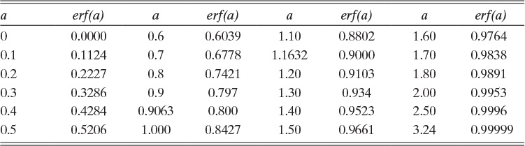
Note that when z = us,i t, which is solute movement solution, argument of the error function is 0, erf is 0, and ci/cF,i = ½. Thus, solute movement theory predicts the center of the spreading wave.
Equation (19-69) is the solution for the breakthrough curve for linear isotherms. Example 19-9 illustrates that the result is an S-shaped curve, which matches experimental results. S-shaped breakthrough curves are also predicted by other solutions for linear sorption systems (e.g., Carta, 1988; Rosen, 1954).
An effective axial dispersion constant Eeff,i is employed in Eqs. (19-67) and (19-69), since it includes effects of both mass transfer and axial dispersion. Under most experimental conditions, mass transfer resistances are important and axial dispersion effects are rather small. If we use ED predicted from Chung and Wen correlation Eq. (19-61), wave spreading will be significantly underpredicted by Eq. (19-69). How do we determine an effective axial dispersion coefficient? Dunnebier et al. (1998) compared solutions that included mass transfer and axial dispersion to results of the Lapidus and Amundson solution. The effective axial dispersion coefficient can be estimated from
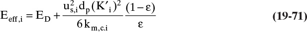
where we have assumed that qi and ci are in same units and K′i is dimensionless. If qi and ci are in different units, then appropriate density (or densities) need to be included with K′i [procedure is similar to that used to derive Eqs. (19-14a) and (19-14b)]. Value of km,c,i can be estimated from Eqs. (19-58) to (19-60), since km,c,i = K′i km,q,i. For linear systems Lapidus and Amundson solution with Eeff.i gives identical results as solutions of Eqs. (19-55) and (19-57a).
19.7.2 Superposition in Linear Systems
Another characteristic of linear systems is that superposition is valid. In other words, solutions can be added and subtracted to give the solution for a combined process. Note that superposition is not valid for nonlinear isotherms. This was illustrated in Example 19-7 where two shock waves combined to form a single shock wave. For linear systems the two waves remain separate and form a staircase arrangement.
We have already employed superposition in some examples. In Example 19-2 we solved a linear chromatography system for separation of anthracene and naphthalene. This solution was derived by obtaining solution for anthracene and solution for naphthalene and then superimposing these two solutions (Figure 19-6). We inherently assumed the two adsorbates are independent. This type of procedure cannot usually be applied to nonlinear systems, since solutes interact [e.g., as shown by the multicomponent Langmuir isotherm, Eq. (19-8)].
Figure 19-6 also illustrates another aspect of superposition. The first step increase for naphthalene in Figure 19-6 is the breakthrough solution (a feed of concentration cF is introduced to an initially clean column) using solute movement theory for a system with a linear isotherm. If we define Xbreakthrough,i as solution for breakthrough with linear isotherms, then for a column that initially has no solute, solution is
Solution to a step-down in feed concentration from cF,i to zero is feed concentration minus breakthrough solution. Based on superposition this solution is loaded column concentration [ci (z,t) = cF,i] minus breakthrough solution Xbreakthrough,i started at time t = telution. Thus at outlet (z = L),
Although solutions including mass transfer and/or dispersion are more complicated than simple solute movement solutions shown in Figure 19-6, the superposition principle remains valid for any linear system. Thus Eq. (19-73) is valid for any linear system if Xbreakthrough,i is any solution for breakthrough with linear isotherms, including solution in Figure 19-6 or in Eq. (19-69). For example, the Lapidus and Amundson solution for elution of a column fully loaded at a fluid concentration of cF,i using pure solvent to remove adsorbate can be determined from Eqs. (19-69) and (19-73):
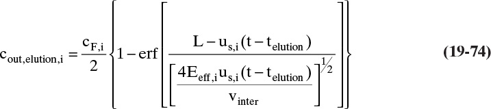
Superposition provides this result with little effort.
As another example, suppose a pulse of feed is input at t = tstart and stopped at t = tend, and pure solvent is fed to the column after stopping the pulse. Solution for this pulse is breakthrough solution (step-up from t = tstart) minus a breakthrough solution (step-down from t = tend):
The period of this pulse is tF = tend – tstart. Any solution for breakthrough for linear isotherms, such as Eq. (19-69), can be substituted into Eq. (19-75).
EXAMPLE 19-9. Lapidus and Amundson solution for elution
A column is packed with ion exchange resin in Ca+2 form. Initially column is saturated with glucose at 10.0 g/L. It is then eluted with pure water starting at t = 0 at a velocity, vinter = 20 cm/min. Column: L = 75.0 cm, Dcol = 4.0 cm. Properties: εe = 0.39, εp = 0, Eeff,i = 5.0 cm2/min, and Kd,i = 1.0. Determine elution curve.
A. Define. Plot cout vs. time.
B, C. Explore and plan. Note that this problem is not ion exchange but is a chemical complexing of glucose with Ca+2 on the resin. Equilibrium data are given in Table 19-2, q = 0.51c. For step down (elution) Lapidus and Amundson solution is given by Eq. (19-74) where us is given by Eq. (19-15b) but without ρp term (because q and c are in same units).
D. Do it. Solute velocity is
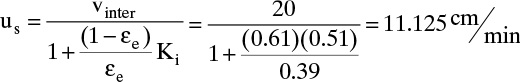
From Eq. (19-74) argument  where telution = 0.
Thus, 
Given a table of values, the easiest solution method is to pick a value of the argument “a” listed in the table and then calculate cout and t for this value. For example, if we select a = 0, which is in Table 19-7,
The equation for time becomes

For the general case (a ≠ 0) we can solve for t either directly or by multiplying both sides of Eq. (A) by (t1/2) and rearranging:
3.3354(t1/2)2 – a(t1/2) – 22.486 = 0
For example, if a = 0.4 [from Table 19-7 erf (0.4) = 0.4284], we find t = 6.437 min. Then
Continuing similar calculations for other “a” values, we generate the following table and the curve in Figure 19-21.
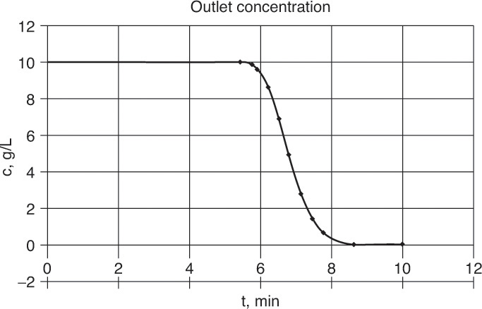
FIGURE 19-21. Outlet concentration profile for Example 19-9

E. Check. The center of the pattern (c = cF/2 for this symmetric curve) should occur at the time calculated by the solute movement solution.
Thus, overall mass balance checks.
F. Generalization. The symmetric S-shaped curve shown in Figure 19-21 is characteristic of linear systems. In linear systems, elution curve (Fig. 19-21) and breakthrough curve (feed to a clean column) are also symmetric. The shape of a breakthrough curve can be seen if the page is flipped over and you look through the paper’s backside. This transformation comes from comparison of the elution solution, Eq. (19-74), with the breakthrough solution, Eq. (19-69). Since Excel supports error functions, solutions using a spreadsheet are convenient.
19.7.3 Linear Chromatography
In analytical chemistry, elution chromatography is employed with very small feed pulses. Thus concentrations are invariably very low and isotherms are almost always linear. For differential pulses (tF is very small compared to time required to elute components), the Lapidus and Amundson solution, Eq. (19-75), can be simplified to (Wankat, 1990)

where t is time after pulse is fed to the column. Equation (19-76), Gaussian solution for linear chromatography, is extensively used to predict analytical chromatography outcomes. Outlet concentrations are determined by setting z = L. Maximum peak outlet concentration occurs at z = L and t = L/us,i
The classic paper by Martin and Synge (1941) on liquid-liquid chromatography used an equilibrium-staged model with linear isotherms for the chromatographic column. Comparison of staged solutions with Eq. (19-76) shows that number of stages Ni is
where PeL,i is the Peclet number based on the column length.
Ni is also related to L through height of an equilibrium plate (HETPi).
These results allow us to calculate the value of Ni or HETPi if Eeff is known, or vice-versa, calculate Eeff if Ni or HETPi is known. This conversion is useful, since easy methods to estimate Ni from chromatographic results are available (see Example 19-10 and homework problems). However, the staged model is awkward, since the number of stages Ni and HETPi for each component can be different. Since chromatography is usually used for relatively difficult separation of similar compounds, the effective axial dispersion coefficients from Eq. (19-71) are often quite close to each other. Thus use of average values results in little error.
The Gaussian solution can be written in shorthand notation as
where xi is the deviation from the location of the peak maximum and σi is the standard deviation. The terms for xi and σi must be in the same units—time, length, or volume. For example, in time units

and in length units

where tR,i is the molecule’s retention time, tR,i = L/us,i.
In linear systems the variances (σi2) from different sources add. This is equivalent to stating that the amount of zone spreading from different sources is additive. Mathematically, this ability to add variances is the reason we can use an effective diffusion coefficient to model a system where mass transfer resistances are important.
Equations (19-79) and (19-80a) can be used to analyze experimental peaks, which are essentially plots of concentration vs. time, to determine us,i and Ni. From Eq. (19-79) the peak maximum must occur when xt,i = 0. Since the outlet concentration profile is being measured at x = L, from Eq. (19-80a), the peak maximum occurs when tmax,i = tR,i = L/us,i, which is identical to solute movement result. Thus us,i and an experimental value for equilibrium constant Ki′ can be determined from time the peak maximum exits the column. This procedure is illustrated in Example 19-10.
Ni can be determined from (Bidlingmeyer and Warren, 1984; Giddings, 1965; Jönsson, 1987; Wankat, 1990)
where peak maximum and width are measured in time units. The constant depends on what width is used. The easiest derivation uses the width as the distance between intersections of the two tangent lines with the base line, which is 13.4% of the total height. The simplest width to use experimentally is pulse width at the half height (ci = cmax,i/2):
The standard deviation σt,i of an experimental Gaussian peak can be estimated from
There are a number of other methods for determining Ni and σt,i of Gaussian peaks (Bidlingmeyer and Warren, 1984; Giddings, 1965; Jönsson, 1987; Wankat, 1990) that all give essentially the same results, although the method presented here is less sensitive to peak asymmetry than some of the other methods (Bidlingmeyer and Warren, 1984). The use of these equations is illustrated in Example 19-10.
The purpose of chromatography is to separate different compounds. Separation occurs because compounds travel at different solute velocities. At the same time, axial dispersion and mass transfer resistances spread peaks. If two peak maxima are separated by more than the spreading of the two peaks, they are said to be resolved. As a measure of how well the peaks are separated, chromatographers use resolution, defined as (Giddings, 1965; Jönsson, 1987; Wankat, 1990)
where tR,A and tR,B are retention times when peak maxima exit. When R = 1.0, the two peak maxima are separated by 2(σt,A + σt,B) ≈ 4σt, and there is about a 2% overlap in the two peaks. An R = 1.5 is considered to be complete baseline resolution of the two peaks.
Resolution can be predicted by substituting expressions for retention times and standard deviations in Eq. (19-82). Assuming the N values are the same for the two components (a reasonable assumption, since resolution is usually calculated for similar compounds), the resulting fundamental equation of chromatography (Giddings, 1965; Wankat, 1990) is

This equation indicates how we can increase resolution if separation is inadequate. For example, increasing column length, which linearly increases N according to Eq. (19-78a), increases resolution by a factor of L1/2. More effect can be obtained by changing equilibrium isotherms (Schoenmakers, 1986) to increase distance between peaks (see Problem 19.B3) or by decreasing particle diameter, which according to Eq. (19-71) decreases Eeff,i, thereby increasing N in Eq. (19-78b).
EXAMPLE 19-10. Determination of linear isotherm parameters, N, and resolution for linear chromatography
A chromatogram is run in a preparative chromatographic system to separate acetonaphthalene (AN) from dinitronaphthalene (DN). Results are shown in Figure 19-22. Find K′AN, K′DN, N, and resolution. K′ values should be in units m3/kg adsorbent = L/g adsorbent.
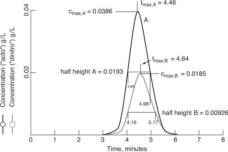
FIGURE 19-22. Analysis of linear chromatography peaks for Example 19-10
Data: L = 50.0 cm, solvent flow rate = 100.0 cm3/min, pulse time = 0.02 minutes, feed concentration AN = 2.0 g/L, feed concentration DN = 1.0 g/L, internal diameter of column = 2.0 cm, εe = 0.4, εp = 0.46, Kd,i = 1.0, ρs = 2222 kg/m3.
Solution
A. Define: Find K′AN, K′DN, N and Resolution.
B. and C. Explore and plan. We can use peak maxima in Figure 19-22 to find times for the two peak maxima, tmax,i. Solute velocities can then be determined as us,i = L/ tmax,i. This allows us to determine K′AN and K′DN by solving Eq. (19-15a) for K′ values:
Ni for each solute can be calculated from Eqs. (19-81a) and (19-81b). Since width at the half height is easier to measure, we use this approach. Determine resolution from Eq. (19-82) using Eq. (19-81c) to estimate values of σAN and σDN.
D. Do it. The values of the peak maximum concentrations and the half height values are given in Figure 19-22.
Solute velocity is
us,AN = L/ tmax,AN = 50.0 cm/ 4.46 min = 11.21 cm/min.
Interstitial velocity is
vinter = vsuper /εe = volumetric flow rate/(π D2/4) /εe = (100 cm3/min)/(π (2.0 cm)2/4)/0.4 = 79.58 cm/min
Then K′AN can be determined from Eq. (19-84):
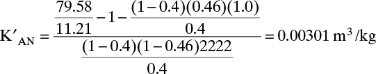
Combining Eqs. (19-81a,b), we have

From Eq. (19-81c)
σAN = 0.425 (4.96 – 3.99) = 0.412
Similar calculations give K′DN = 0.00316, NDN = 117, and σDN = 0.429.
Resolution can be calculated from Eq. (19-82):

E. Check: The values of K′ are within 2% of literature values, K′AN = 0.00306 and K′DN = 0.00322.
F. Generalization: This is a very low resolution, which agrees with Figure 19-22, since peaks are clearly not separated. To obtain better resolution in an analytical system, much smaller particles would probably be used to drastically increase N. An alternative is to use a different chromatographic packing that has a higher selectivity. In a preparative system these methods could be employed and column length would probably be increased.