
Chapter 18. Introduction to Membrane Separation Processes
This chapter presents an introduction to the four membrane separation methods most commonly used in industry: gas permeation, reverse osmosis (RO), ultrafiltration (UF), and pervaporation (pervap). These membrane separation processes are based on the rate at which solutes transfer though a semipermeable membrane. They are not operated as equilibrium-staged processes. The key to understanding these membrane processes is the rate of mass transfer, not equilibrium. Yet, despite this difference, we will see many similarities in the solution methods for different flow patterns with the solution methods developed for equilibrium-staged separations. Because the analyses of these processes are often analogous to the methods used for equilibrium processes, we can use our understanding of equilibrium processes to help understand membrane separators.
Because membrane processes are usually either complementary or competitive with distillation, absorption, and extraction, some knowledge of the membrane separations will prove very helpful even if the engineer usually uses equilibrium-based processes. In gas permeation components selectively transfer through the membrane. Gas permeation competes with cryogenic distillation as a method to produce nitrogen. Absorption and gas permeation are competitive methods for removing carbon dioxide from natural gas streams. In RO a tight membrane that rejects essentially all dissolved components is used. Water dissolves in the membrane and passes through under a pressure difference up to 6000 kPa (800 psi) (Li and Kulkarni, 1997). RO has in many cases displaced distillation as a method for desalinating seawater and is extensively used to make wastewater potable (Reisch, 2007). UF membranes are fabricated to pass low molecular weight molecules and to retain high molecular weight molecules and particulates. The pressure difference, 70 to 1400 kPa (10–100 psi) is more modest than in RO. UF is a useful method for separating proteins and other large molecules that essentially have no vapor pressure and, thus, cannot be distilled. UF competes with extraction, crystallization, and chromatography as a separation method for biochemicals. In pervap the feed is a liquid, while the permeate product is removed as a vapor. Pervap is used as a method to break azeotropes and is often coupled with distillation columns. Since membrane separations are based on different physicochemical properties than equilibrium-staged separations, membrane separators can often perform separations such as separation of azeotropic mixtures and separation of nonvolatile components, which cannot be done by distillation or other equilibrium-based separations. Descriptions of these membrane separation processes are found in Baker (2012), Baker et al. (1990), Eykamp (1997), Geankoplis (2003), Kucera (2010), Noble and Stern (1995), Ho and Sirkar (1992), Strathmann (2011), Wang and Zhou (2013), and Wankat (1990).
There are several other membrane processes that are in commercial use but are not covered in this chapter. In dialysis, small molecules in a liquid diffuse through a membrane because of a concentration driving force (Strathmann, 2011). The major applications are hemodialysis and the artificial kidney developed by Kolff and Beck in 1944 for treatment of people whose kidneys do not function properly (Lonsdale, 1982). Electrodialysis (ED) uses an electrical field to force cations through cation exchange membranes and anions through anion exchange membranes (Lonsdale, 1982; Strathmann, 2011). The membranes are alternated in a stack, and every alternate region becomes concentrated or diluted. ED is used for desalination of brackish water and in the food industry. Vapor permeation is similar to gas permeation except vapors that are easily condensed are processed (Huang, 1991). This process has not met its potential partly because of difficulties with condensation of liquid. Liquid membranes use a layer of liquid instead of a solid polymer to achieve the separation (Wankat, 1990). Liquid membrane systems can be operated as countercurrent processes, and, to some extent, compete with extraction. Microfiltration is similar to UF but is used for particles between the sizes processed by UF and normal filtration (Noble and Terry, 2004). Nanofiltration removes molecules and particles that are in-between the sizes removed by RO and UF (Strathmann, 2011). The design procedures developed for RO and UF can be applied to microfiltration and nanofiltration. The entire spectrum of membrane separations is summarized in Table 18-1. Nanofiltration is not listed separately but is similar to RO except that Δp is from 0.3 to 3.0 MPa, and the approximate size retained is 8-50Å.
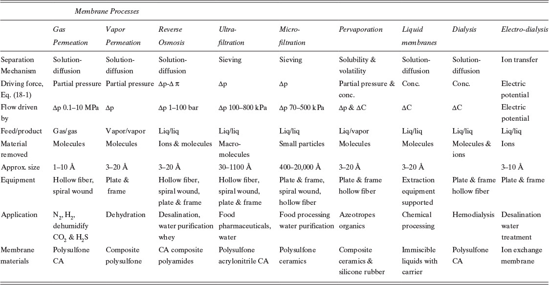
Key: CA = cellulose acetate
TABLE 18-1. Properties of membrane separation systems (Drioli and Romano, 2001; Noble and Terry, 2004; Wang and Zhou, 2013; Wankat, 1990)
At the level of this introduction the mathematical sophistication needed to understand membrane processes is approximately the same as that needed for the equilibrium-staged processes. A background in mass transfer (Chapter 15) is helpful but not essential.
Note: A nomenclature list for this chapter is included in the front matter of this book.
18.0 Summary—Objectives
In this chapter we study membrane separations including gas permeation, RO, UF, and pervaporation. At the end of this chapter you should be able to satisfy the following objectives:
1. Explain differences and similarities between the different membrane separation systems
2. For a perfectly mixed system with no concentration polarization, predict performance of an existing membrane separation system, and design a new membrane separation system using both analytical and graphical analysis procedures
3. Explain and analyze the effect of concentration polarization, and include it in the design of perfectly mixed membrane separators
4. Explain and analyze the effect of gel formation, and include it in the design of UF systems
5. Determine appropriate operating conditions for pervaporation systems
6. Explain and analyze effects of flow patterns on separation achieved in membrane systems
18.1 Membrane Separation Equipment
A membrane is a physical barrier between two fluids (feed side and product side) that selectively allows certain components of the feed fluid to pass. The fluid that passes through the membrane is called permeate, and the fluid retained on the feed side is called retentate. The equipment needed for separation is deceptively simple. It consists of the membrane plus a container to hold the two fluids. The simplest arrangement is a stirred tank that is separated into two volumes via a membrane. Stirred-tank systems are used in laboratories but not commonly in large-scale separations.
Common commercial geometries are shown in Figure 18-1 (Leeper et al., 1984). More extensive construction details are shown by Baker et al. (1990) and Eykamp (1997). The plate-and-frame system (Figure 18-1A) is similar to a parallel-plate heat exchanger or a plate-and-frame filter press, except that the filter cloth is replaced by flat sheets of membranes. This design is used for food-processing applications in which rigorous cleaning by disassembly may be required, for electrodialysis (which involves passing a current through the membrane), and for membrane materials that are difficult to form into more complicated shapes.
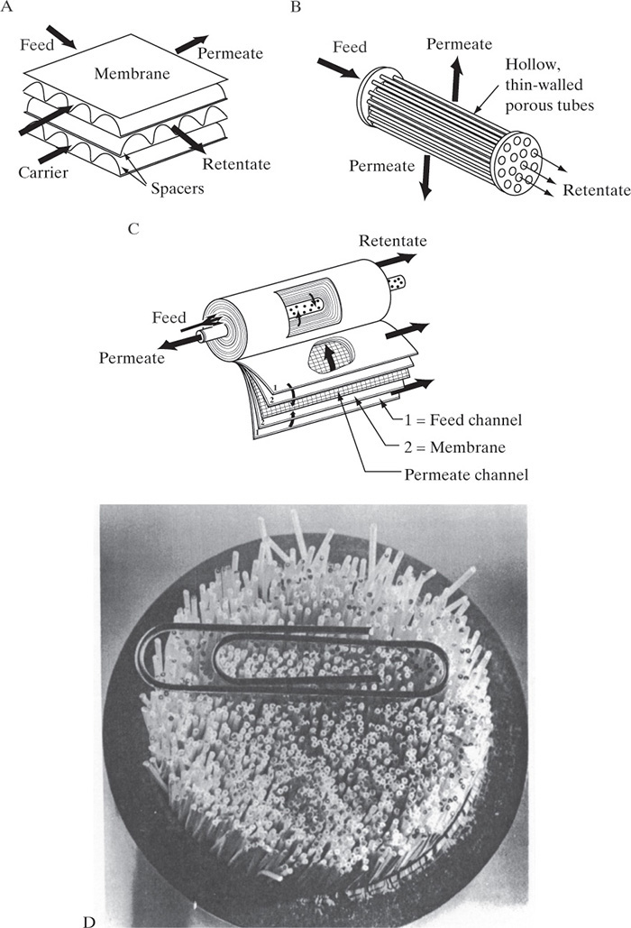
FIGURE 18-1. Schematic diagrams of common industrial membrane modules; (A) plate and frame, (B) tube in shell, (C) spiral wound, (D) details of hollow-fiber module. Reprinted from Leeper et al. (1984), pp. 36–37.
The tube-in-shell system (Figure 18-1B) is occasionally used. This configuration is very similar to a shell-and-tube heat exchanger. The membrane is coated on a porous support. The main advantage of these systems is that they can be cleaned by passing sponge balls through the separators. The surface area per unit volume is larger than plate and frame but smaller than spiral wound.
The spiral-wound configuration (Figure 18-1C) is more complicated but has a significantly larger surface area per unit volume. With proper design of the channels there is significant turbulence at the membrane surface that promotes mass transfer. The spiral-wound configuration is the most common module for RO because it has a high surface area/volume and does not become easily clogged with particulates. These systems have also been used for carbon dioxide recovery and UF of relatively clean solutions.
The hollow-fiber configuration (Figure 18-1D) looks schematically very similar to the tube-in-shell system, except the tubes are replaced by a very large number of hollow fibers made from the membrane. This configuration has the largest area-to-volume ratio. The hollow fibers can be optimized for a particular separation. For RO the inner diameter is about 42 microns, and the outer diameter is about 85 microns. The separation is done by a 0.1 to 1 micron skin on the outer surface. The remainder of the membrane is a structural support. For gas permeation the requirement of a small pressure drop inside the tubes dictates a larger inner-fiber diameter. For UF, in which feed can be dirty, the fibers are 500 to 1100 microns inside diameter. Typically the feed is inside the tubes, and the thin membrane skin is on the inside of the fibers. Care must be taken that particulates do not clog the fibers. Hollow-fiber membranes are technologically the most difficult to make.
The most common systems are spiral wound and hollow fiber. Systems are usually purchased as off-the-shelf modules in a limited number of sizes. Since a standard size is unlikely to provide the required separation and flow rate for a given problem, a series of modules is cascaded to obtain the desired separation (Figure 18-2). The parallel configuration (Figure 18-2A) allows one to increase the feed flow rate and is used with all of the membrane separations. Parallel operation is roughly analogous to increasing the diameter of a distillation or absorption column, except there is very little economy of scale [the exponent in Eq. (11-3) is ∼1].
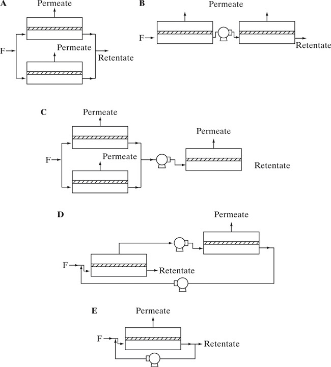
FIGURE 18-2. Membrane cascades; (A) parallel, (B) retentate in series, (C) parallel and series, (D) permeate in series, (E) retentate recycle or feed and bleed
The retentate-in-series system (Figure 18-2B) increases the purity of the more strongly retained components and simultaneously increases the recovery of the more permeable species. Unfortunately, purity of permeate and recovery of retained components both decrease. This configuration is used for production of less-permeable nitrogen from air at relatively high pressure since the nitrogen has not permeated through the membrane. The system is roughly analogous to a crossflow extractor or stripper. Parallel and retentate-in-series systems are often combined (Figure 18-2C).
The permeate-in-series system (Figure 18-2D) is used when the permeate product is not of high enough purity and one or more additional stages of separation are required. Designers try to avoid this configuration if possible. The major cost of operating most membrane separators is the energy required to create the pressure difference to force the permeate through the membrane. This configuration requires an additional compressor or pump to repressurize the permeate for the next membrane separator. One of the major disadvantages of membrane separators is that additional stages for the permeate do not reuse the energy-separating agent (pressure). The equilibrium-staged separations have the advantage that energy-separating agents (heat and cooling) can easily be reused. Ideally, a commercial membrane will be available that produces permeate of the desired purity in one stage.
A final common membrane cascade is the retentate-recycle or feed-and-bleed mode (Figure 18-2E). The recycle allows for a very high flow rate in the membrane module to increase mass transfer rates and minimize fouling. The same high flow rates can be obtained without recycle, but a very long membrane system is required to have a sufficiently long residence time. Recycle is used extensively with continuous and batch UF systems. Recycle in Figure 18-2E is similar to recycle in Figure 18-2D since high-pressure retentate is recycled in both cases. Thus, the compressor or pump needs only to boost pressure (e.g., because of friction losses for flow inside a hollow-fiber membrane), not overcome the large pressure difference that results when fluid permeates through the membrane.
The flow patterns on the retentate (feed) and permeate sides of the membrane have major effects on the mass balances and the separation. These flow patterns can be perfectly mixed on both sides, plug flow on one side and perfectly mixed on the other side, plug flow in the same direction on both sides (cocurrent), plug flow in opposite directions on the two sides (countercurrent), mixed on one side and crossflow on the other, and somewhere in between these ideal regimes. For example, if we consider the hollow-fiber module shown in Figure 18-1D, the flow inside the hollow fibers is very close to plug flow. Depending on the shell-side design, the flow on the shell side could be an approximately well-mixed, cocurrent plug flow or a countercurrent plug flow. Countercurrent plug flow usually gives the most separation.
To simplify the mathematics, in Sections 18.2 to 18.6 we assume that both sides of the membrane are perfectly mixed. The resulting designs are conservative in that the actual apparatus results in the same or better separation than predicted. The effect of other flow patterns is explored in Section 18.7.
18.2 Membrane Concepts
Clearly the key to membrane separators is the membrane. The membrane needs to have a high permeability for permeate and a low permeability for retentate. It helps if the membrane has high temperature and chemical resistances, is mechanically strong, resists fouling, can be formed into the desired module shapes, and is relatively inexpensive. Commercial membranes are made from polymers, ceramics, and metals (e.g., palladium for helium purification), but polymer membranes are by far the most common. Membrane development is done by a few large chemical companies and several specialty firms. Most chemical engineers use membrane separators, but they are never involved in membrane development. However, some understanding of the polymer membrane is useful when specifying and operating membrane separators.
A large number of polymers (Figure 18-3) have been used to make membranes for membrane separators. Cellulose, ethyl cellulose, and cellulose acetate (actually a polymer blend of cellulose, cellulose acetate, and cellulose triacetate [Kesting and Fritzsche, 1993]) were the first commercially successful membranes and are still used. These materials have relatively poor chemical resistance, but their low cost makes them attractive when they can be used. The most common commercial membrane material is polysulfone, which has excellent chemical and thermal resistance. Various polyamide polymers are also commonly used in RO. Silicone rubber, which has very high fluxes but low selectivity, is often used in pervaporation to preferentially permeate organics and as a coating on composite membranes for gas permeation. A large variety of grafted polymers, specialty polymers, and composite membranes has been developed to optimize flux and selectivity, particularly for pervaporation (Huang, 1991; Strathmann, 2011) but also other membrane separations. Kesting and Fritzsche (1993) are an excellent source for information on the relationship between polymer structure and membrane properties for the polymers used for gas separation.
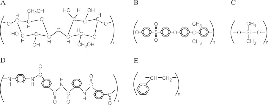
FIGURE 18-3. Monomers for polymers used to form membranes; (A) cellulose (GP, RO, UF), (B) polysulfone (GP, RO, UF), (C) silicone rubber from dimethyl siloxane (GP, pervaporation), (D) example of polyamide (RO, UF), (E) polystyrene (matrix for composite resins, pervaporation) (Kesting and Fritzsche, 1993; Wankat, 1990).
The basic equation for flux of permeate through the membrane is

Although this equation is derived from experiments and is not a fundamental law, it is so basic and powerful that you need to memorize it and explore its implications in as many ways as possible. The exact form of the equation depends on the type of flux and the type of separation.
The flux can be written as a volumetric flux,
or as a mass flux,
or as a molar flux,
These fluxes are obviously related to each other:
where ρm and ρ are molar and mass densities, respectively. Once flux is known, it is used in conjunction with feed rate and feed concentration to determine the membrane area required.
Equation (18-1a) can be used to determine flux once appropriate terms on the right-hand side of the equation are known. Permeability, P, is a transport coefficient that can be determined directly from experiment. In some cases permeability can be estimated from more fundamental variables such as solubility and diffusivity (see next section). The membrane separation thickness, tms, is the thickness of the portion of the membrane that is actually doing the separation. This is often a thin skin with a thickness less than 1 micron (10–6 m) and, in polymeric hollow-fiber gas permeation membranes, can be as low as 0.1 micron. Since tms can be difficult to measure, the ratio (P/tms), the permeance, is often reported from experimental data. The units of P and (P/tms) depend on the flux and driving force employed.
The driving force depends on the type of membrane separation. For gas permeation the driving force is the difference in partial pressure of the transferring species across the membrane. For RO the driving force is the pressure difference minus the osmotic pressure difference across the membrane. For UF the driving force is the same as for RO but usually simplifies to pressure difference across the membrane since osmotic pressures are small. These driving force effects are specific to each membrane separation and are discussed in more detail in later sections.
Since flux is flow rate per membrane area, increasing flux (while maintaining the desired separation) decreases membrane area. The result is a more compact, less expensive device. Equation (18-1a) shows that flux can be increased by increasing permeability or driving force or by decreasing the separation thickness. Permeability of the membrane depends on interactions between the molecular structure of the membrane material and the solutes. These effects are briefly discussed in the sections on each membrane separation. More details on molecular structure-permeability effects are in the books by Baker (2012), Kesting and Fritzsche (1993), Ho and Sirkar (1992), Noble and Stern (1995), and Strathmann (2011).
For many years attempts were made to make very thin membranes, but there was always difficulty in making the membranes mechanically strong enough. Sidney Loeb and Srinivasa Sourirajan (1960, 1963) made the breakthrough discovery. They found that anisotropic (asymmetric) membranes with a very thin skin (0.1 to 1 µm) on a much thicker porous support have the necessary mechanical strength while having a very small separation thickness. Schematics of isotropic and anisotropic membranes are shown in Figure 18-4. Another method for producing an asymmetric membrane is to cast a thin layer of one polymer onto a porous supporting layer of another polymer to form a composite membrane. Although not all membrane separators use asymmetric membranes, they are the most common.
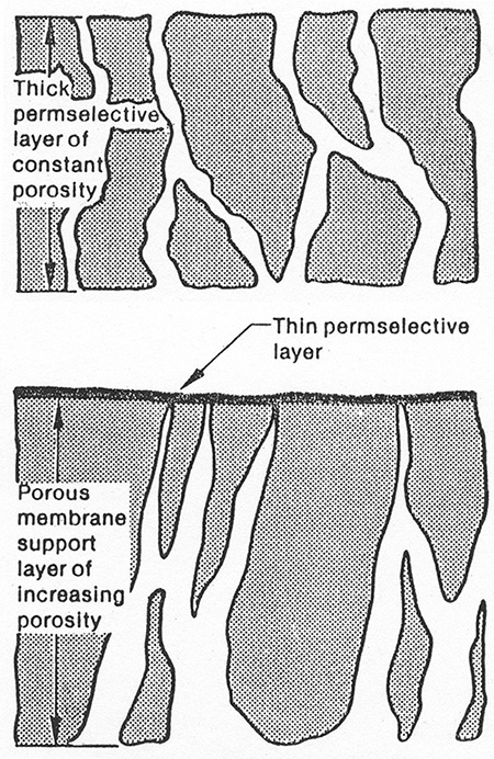
FIGURE 18-4. Schematics of (A) isotropic and (B) anisotropic membranes, reprinted from Leeper et al. (1984)
Membranes must be essentially totally hole free. If there is a pinhole high-pressure fluid will be pushed through in convective flow. This fluid has not undergone the separation process and will contaminate the product. Example 18-4 calculates the magnitude of this hole effect.
18.3 Gas Permeation
We will consider gas permeation first, since, in addition to being commercially important, in many ways gas systems are closest to being ideal. Once ideal operation is understood, we can look at deviations from ideality for other membrane separations. Gas permeation membrane systems are used commercially for separation of permanent gases. Some common applications are purification of helium, hydrogen, and carbon dioxide; production of high-purity nitrogen from air; and production of air enriched in oxygen (low-purity oxygen).
Gas permeation systems typically use hollow-fiber or spiral-wound membranes, although hollow-fiber systems are more common (Baker, 2004). Cellulose acetate membranes are used for carbon dioxide recovery, polysulfone coated with silicone rubber is used for hydrogen purification, and composite membranes are used for air separation. Feed gas is forced into the membrane module under pressure. Retentate, which does not go through membrane, becomes concentrated in less permeable gas. Retentate exits at a pressure that is close to inlet pressure. More permeable species are concentrated in permeate. Permeate, which has passed through the membrane, exits at low pressure. Operating cost for a gas permeator is the cost of the compression of feed gas and the irreversible pressure difference that occurs for gas that permeates the membrane. A typical hollow-fiber unit contains 5000 m2 membrane area per m3 at a cost of approximately $200/m2.
For gas permeation steady-state overall flux Eq. (18-1a) written for volumetric flux of gas A becomes
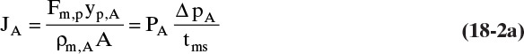
where JA is volumetric flux of gas A, Fm,p is molar transfer rate of permeate (gas that has permeated through membrane), yp,A is mole fraction A in the permeate, ρm,p,A is molar density of solute A in permeate, A is membrane area available for mass transfer, PA is permeability of species A, driving force for separation ΔpA is difference in partial pressure of A across membrane, and tms is thickness of membrane skin which actually does the separation. Ratio (PA/tms) is called permanence and is often a variable that is measured experimentally. Since partial pressure = (mole fraction)(total pressure) or pA = yAp, Eq. (18-2a) can be expanded to

where pr is the total pressure on the retentate (high pressure) side, yr,w,A is mole fraction A on the retentate side at the membrane wall, and pp and yp,w,A are pressure and mole fractions at the wall on the permeate (low pressure) side. The flux equation for other components will look exactly the same as for component A, except subscript A will be changed to B, C, . . . as appropriate. Mole fractions at the membrane wall depend on flow patterns and mass transfer rates in the membrane module (Sections 18.3.2 and 18.7).
18.3.1 Gas Permeation of Binary Mixtures
Commercial separation of binary mixtures by gas permeation is common. In binary mixtures
where y without subscript A or B refers to the mole fraction of faster permeating species A. In a binary system, flux of slower moving component B is

Since pressure and mole fractions can vary along the membrane, in principle Eqs. (18-2a) to (18-2c) are applied point by point along the membrane. In almost all systems there is no concentration gradient on the permeate side perpendicular to the membrane; thus, we normally replace yp,w,A with yp,A, which can vary along the membrane. In addition, if mass transfer on the retentate side is not rapid, the mole fractions and partial pressures at the membrane surface will not be the same as in bulk gas or feed gas (see concentration polarization in Section 18.4). Usually mass transfer rates in gas systems are high enough that the mole fraction at the membrane surface is almost equal to the mole fraction in bulk gas.
Most gas permeation membranes work by a solution-diffusion mechanism. On the high-pressure side of the membrane, gas first dissolves into the membrane. It then diffuses through the membrane’s thin skin to the low-pressure side where the permeate reenters the gas phase. For this type of membrane, permeability is the product of gas solubility HA in the membrane times diffusivity DA,M in the membrane:
Solubility parameter HA is very similar to a Henry’s law coefficient. Representative permeabilities for several polymer membranes are shown in Figure 18-5 and in Table 18-2. Small molecules such as helium have high diffusivities but low solubilities, while large gas molecules such as carbon dioxide have high solubilities but low diffusivities. The resulting product, permeability P, is relatively large for both small and large molecules but has a minimum for molecules around the size of nitrogen.
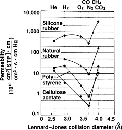
FIGURE 18-5. Permeation of gases in polymer membranes (Baker and Blume, 1986), reprinted with permission from Chem. Tech., 232 (1986), copyright 1986, American Chemical Society.
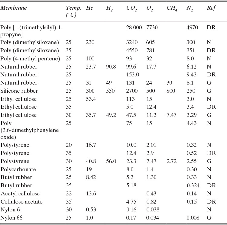
TABLE 18-2. Permeabilities of gases in various membranes; cm3(STP)cm/[cm2.s.cm Hg] × 1010; reference code: N = Nakagawa, 1992; DR = Drioli and Romano, 2001; G = Geankoplis, 2003
If driving forces are equal, gases with higher permeabilities transfer through membranes at higher rates. It is useful to define selectivity αAB as
which can be used as a short-hand method of comparing ease of separation of gases. Selectivity of two solutes can be estimated from Figure 18-5 and Table 18-2. For example, from Figure 18-5, αCO2∇N2 = PCO2 / PN2 = 24/0.3 = 80 in a CA membrane. Selectivity is a function of concentration, pressure, and temperature since individual permeabilities depend on these variables. However, αAB tends to be less dependent on these factors than individual permeabilities. Note that αAB is analogous to relative volatility defined in Chapter 2. Since gas permeation is usually operated as one-stage systems, αAB values of 20.0 and higher are preferred instead of the much more modest values commonly employed in distillation.
Robeson (1993) found an upper limit to performance of polymer membranes in the commercially important separation of oxygen and nitrogen from air. On a log-log plot of selectivity versus oxygen permeability (a Robeson plot), the upper bound plots as a straight line (see Problem 18.D17 for details). Although theoretical reasons for this limit have not been found, very few new membranes have been developed that are able to perform better than Robeson’s limit. Membrane research has focused on ways to do better than Robeson’s upper limit.
18.3.2 Binary Permeation in Perfectly Mixed Systems
Mass balances for a gas permeation membrane module that is assumed to be completely mixed on both sides of the membrane have the simplest form since mole fractions and pressures are constant. Equations (18-2) and (18-3b) can then be used in algebraic mass balances, and integration is not required to find the average retentate and permeate mole fractions. Since many gas permeators have high diffusivities and mass transfer rates, we assume mass transfer from bulk fluid to membrane surface is rapid, which makes yr = yr,w (mole fraction of A at membrane wall). These two assumptions also make yr,out = yr = constant and greatly simplify analysis. We obtain a rate transfer (RT) equation by writing Eq. (18-2) for transfer through membrane for both more-permeable and less-permeable species, solving both equations for permeate flow rate, and setting equations equal to each other. From Eq. (18-2c), the transfer equation for more permeable component A is

while from Eq. (18-3b) for less permeable component B in a binary separation

Because permeate is typically at low pressures where gas molecules are far apart, transfer of A is usually independent of transfer of B and vice versa. Thus, PA and PB are constant. Solve both equations for Fm,p, and set them equal to each other.

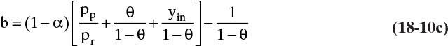
This equation can be solved for either yr or yp, although solving for yr is easier. After some algebra, the result is
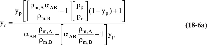
Equation (18-6a), the rate transfer (RT) equation, relates mole fractions in retentate and permeate based on membrane parameters and driving force. Although Eq. (18-6a) was derived for perfectly mixed gas permeators, it is applicable to other flow configurations if applied point by point on the membrane. Since it was derived based on transfer rates, Eq. (18-6a) is not an equilibrium expression; however, it can replace equilibrium expressions for binary systems.
Completely mixed membrane permeators (Figure 18-6) are rate equivalent of flash distillation (Hoffman, 2003). The geometries are identical—a single feed goes into a well-mixed chamber, and two products are withdrawn. The more permeable species concentrates in the permeate product, which is analogous to the more volatile component concentrating in vapor. However, the two products are not in equilibrium but are related by RT Eq. (18-6a). Because of geometric similarity, analysis is surprisingly similar to binary flash distillation analysis.
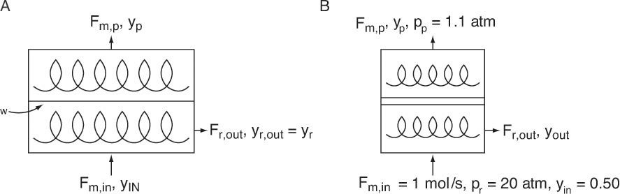
FIGURE 18-6. Completely mixed membrane module; (A) general case, (B) sketch for Example 18-1
The overall mole balance for Figure 18-6 is
and the mole balance on the more permeable component is
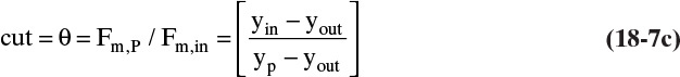
Equations (18-7) can be combined and solved for either yr,out or for yp. Since solving for yp keeps the analogy with flash distillation intact, we will solve for yp. In molar units

Equation (18-8) is an operating equation for well-mixed gas permeators. The ratio θ = (Fm,p/Fm,in), called cut, is an important operating parameter. RT Eq. (18-6a) and operating Eq. (18-8) are the equations needed to solve problems with perfectly mixed, binary gas permeators. Solution is illustrated in Example 18-1 when yp is known and in Example 18-2 when θ is specified.
Once permeate yp and retentate yr mole fractions are known, volumetric fluxes can be determined from Eqs. (18-2b) and (18-3b), and the total volumetric flux is
If the area is known, the molar transfer rate can be determined from
or from
If the molar feed rate is known, then Fm,p = θ Fm,in, and area A is
or from
Gas permeators often operate at temperatures and pressures at which gases are very close to ideal. Ideal gas behavior simplifies calculations. At constant pressure and temperature molar densities of all ideal gases are equal, ρm,A = ρm,B = p/(RT), and densities cancel in Eq. (18-6a). The resulting RT equation is

The volumetric flow rate units of permeabilities listed in Table 18-2 are cm3 (STP)/s. For ideal gases this is equivalent to a molar flow rate since 1.0 mol occupies 22,400 cm3 at standard temperature and pressure (STP). These simplifications are illustrated in Example 18-1.
EXAMPLE 18-1. Well-mixed gas permeation—sequential, analytical solution
A perfectly mixed gas permeation module is separating carbon dioxide from nitrogen using a poly (2,6-dimethylphenylene oxide) membrane. Feed is 20.0 mol% carbon dioxide and is at 25.0°C. Module has 50.0 m2 of membrane. Module is operated with a retentate pressure of 5.5 atm and a permeate pressure of 1.01 atm. We desire a permeate that is 40.0 mol% carbon dioxide (yp = 0.40). Membrane thickness is tms = 1.0 µm = 1.0 × 10⁻⁴ cm. Find yr,CO2 = yr,out,CO2, JCO2, Fm,p (mol/min), cut θ, and Fm,in (mol/min).
Solution
A. Define. This is a simulation problem. We want to find how much gas can be processed by a well-mixed module with a known membrane area at specified operating conditions.
B, C. Explore and plan. Permeabilities of carbon dioxide and nitrogen for this membrane are listed in Table 18-2. Selectivity, αCO2–N2, is the ratio of these permeabilities. yr,CO2 can be found from RT Eq. (18-6b). CO2 volumetric flux JCO2 can be calculated from Eq. (18-2b) and molar permeate flow rate Fm,p from Eq. (18-9c). Cut θ and Fm,in can then be determined from mole balances, Eqs. (18-7).
D. Do it. From Table 18-2:
PCO2 = 75.0 and PN2 = 4.43, both cm3, (STP)cm/[cm2s cm Hg] × 10–10.
Then αCO2–N2 = (75.0 × 10⁻¹⁰)/(4.43 × 10–10) = 16.9.
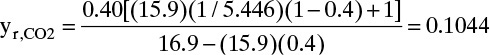
Pressure ratio pr/pp = 5.5/1.01 = 5.446. For ideal gases, a reasonable assumption, ρm,CO2/ρm,N2 = 1.0 and ρm,CO2 = 1.0 mol/22.4 L(STP). Substituting in values with yP = 0.4 in RT Eq. (18-6b), we obtain
CO2 flux can be determined from Eq. (18-2b) for a perfectly mixed module:
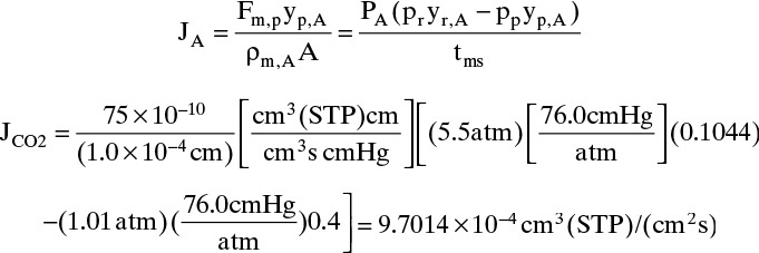
Then Fm,p = JCO2ρm,CO2A / yp,CO2
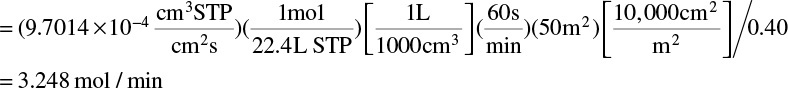
Note ρm,CO2 = (1.0 mol)/(22.4 L) is value of molar density of an ideal gas at STP.
Mole balances can now be solved several different ways. For example, by simultaneously solving Eqs. (18-7a) and (18-7b) we obtain
Then θ = (0.20 – 0.1044)/(0.40 – 0.1044) = 0.3234, and Fm,in = Fm,p θ = 3.248/0.3234 = 10.044 mol/min.
E. Check. Recalculating all numbers gave the same result.
F. Generalize. Notes:
1. Because one of the outlet mole fractions was known, we could calculate the other from the RT equation; thus, simultaneous solution of Eqs. (18-6b) and (18-8a) was not required. If neither outlet mole fraction is known, then simultaneous solution is required (see Example 18-2).
2. Units are obviously very important and should be carried throughout the solution.
3. Using conversion, 1.0 mol = 22.4 L (STP) is equivalent to using the ideal gas law.
4. Solution implicitly assumed there are no pin holes in the membrane that allow convective flow. Example 18-4 analyzes the effect of pin holes on product purity. In effect, membranes have to be almost perfect.
A graphical solution to perfectly mixed gas permeators is straightforward. On a graph of yp vs. yout, Eq. (18-8a) plots as a straight line with a slope of –(1 – θ)/θ. Note that cut θ is analogous to f = V/F in a flash distillation system. Intersection with yp = yout line occurs at yp = yout = yin, which is analogous to y = x = z in a flash system. Intersections with axes can also be determined (see Example 18-2 and Figure 18-7). Simultaneous solution is obtained at the point of intersection of the straight line representing Eq. (18-8a) and the curve representing Eq. (18-6a). This method is illustrated in Figure 18-7 for a number of values of θ (see Example 18-2).
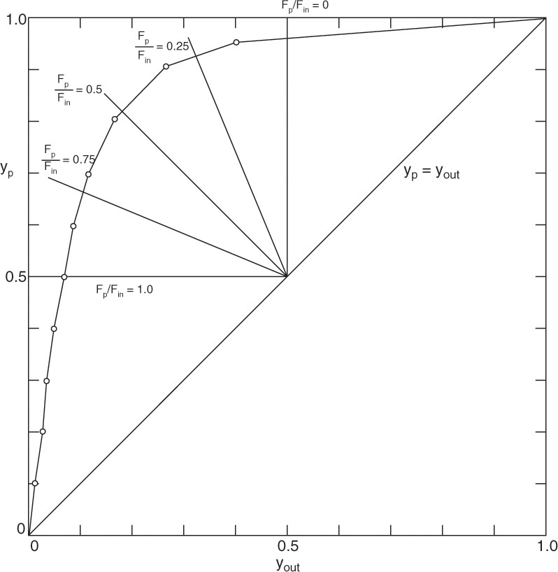
FIGURE 18-7. Graphical solution for well-mixed gas permeation system for Example 18-2
EXAMPLE 18-2. Well-mixed gas permeation—simultaneous solutions
Chern et al. (1985) measured permeabilities of carbon dioxide and methane as PCO2 = 15.0 × 10⁻¹⁰ and PCH4 = 0.48 × 10⁻¹⁰ [cc(STP)cm]/[cm2 s cm Hg] in a cellulose acetate membrane at 35.0°C. Separate a feed gas that is 50.0 mol% carbon dioxide and 50.0 mol% methane at 35.0°C. (Since many natural gas supplies contain CO2 in addition to CH4, this is an important industrial separation problem.) Retentate pressure is pr = 20.0 atm, and permeate pressure is pp = 1.1 atm. A completely mixed membrane module (Figure 18-6) is used.
A. Determine values of yp and yout for cut θ = 0, 0.25, 0.5, 0.75, and 1.0 using analytical (θ = 0.25 only), spreadsheet (θ = 0.25 only), and graphical solutions.
B. If effective membrane thickness is tms = 1.0 µm = 1.0 × 10⁻⁶ m, determine fluxes for θ = 0.25.
C. For θ = 0.25 determine membrane area for a feed gas flow rate of Fm,in = 1.0 mol/s.
Solution
A. Define. The module is sketched in Figure 18-6B. We need to solve equations analytically, on a spreadsheet, and plot a graph that allows us to find yp and yout for different values of θ. When θ = 0.25, find the fluxes of carbon dioxide and methane, and find the membrane area.
B, C. Explore and plan. Selectivity αCO2–CH4 = PCO2/PCH4. We will assume gases are ideal.
Analytical solution: Solve Eqs. (18-6b) and (18-8a) simultaneously.
Spreadsheet solution: Use spreadsheet tool Goal Seek or Solver to find the solution. The advantage is less algebra is required than for analytical solution. However, analytical solution is advantageous when a large number of solutions are needed (e.g., see analysis for crossflow in this chapter’s appendix.
Graphical solution: If we pick values of yp, Eq. (18-6b) can be used to calculate corresponding values of yr for the RT curve. For a well-mixed permeator, the RT curve and operating line, Eq. (18-8a), can then be plotted on an yp vs. yr graph for different values of θ. Since the system is well mixed, points of intersection give solutions for yp and yr = yout. Fluxes can then be calculated from Eq. (18-4).
D. Do it. Preliminary calculations: For ideal gases molar densities are equal, and the ratio of densities is 1.0. Selectivity is
αCO2-CH4 = PCO2/PCH4 = (15.0 × 10⁻¹⁰)/(0.48 × 10–10) = 31.25
pp/pr = 1.1/20.0 = 0.055 (Note that any set of consistent units can be used for this ratio.)
Analytical solution: Solving Eq. (18-8a) for yr,
After substituting Eq. (18-8b) in (18-6b) (in Example 18-1) and doing considerable algebra, we obtain the quadratic equation
where
This quadratic equation can be solved numerically or analytically. An analytical solution is obtained if we use the quadratic formula
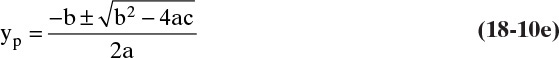
Substituting in values θ = 0.25, α = 31.25, yin = 0.50, and pp/pr = 0.055, we obtain a = 11.747, b = –33.247, c = 20.833, and yp = 0.9365 or 1.894. The second value for yp can be eliminated since the mole fraction cannot be greater than 1.0. yr is found from Eq. (18-8b), yr = 0.3545. Solution of the quadratic equation obtained with a spreadsheet using Goal Seek is identical.
Spreadsheet Solution: Algebra can be eliminated by coding operating equation (18-8b) in one cell and RT equation (18-6b) in another cell. Guess a value of yp, and calculate yr,op eq, yr,RT eq, and test = 1000.0 × (yr,op eq – yr,RT eq). Use Goal Seek to force test = 0 by changing yp.
Graphical Solution: The RT curve, Eq. (18-6b), that relates yr and yp becomes
yr = {[(31.25 – 1.0)(0.055)(1.0 – yp) + 1.0]yp}/[31.25 – 30.25 yp]
The following table for the RT curve is generated by selecting arbitrary values of yp.
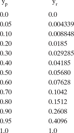
These values are plotted in Figure 18-7 for the RT curve.
a. Operating Eq. (18-8a) intersects the yp = yr line at yr = yin = 0.50. Slope = –[1 – θ]/θ. For example, when θ = 0.25, the slope = –0.75/0.25 = –3.0.
Solutions are at intersections of operating lines and RT curve. For θ = 0.25, Figure 18-7 shows that yp = 0.93 and yr = yout = 0.35. Graphical solution is particularly useful for answering questions that require interpretation. For example, what is lowest value of yout?
b. When θ = 0.25, flux is determined from Eq. (18-4) using yp and yr values from part a:
For CH4 : yp,CH4 = 1–yP = 0.07, yout,CH4 = 1.–0.35 = 0.65

Note that care must be taken with the units.
c. Once volumetric flux is known, we can calculate area from Eq. (18-9d), A = Fm,p/(Jtotal ρm). Since θ = 0.25 and Fm,in = 1.0 mol/s, Fm,p = θ Fm,in = 0.25 mol/s.
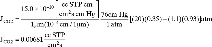
Volumetric flux is, ![]() .
.
Ideal gas molar density ρm = 1.0 mol/22.4 L STP.
Taking care to properly calculate units, membrane area is
E. Check. Analytical, spreadsheet, and graphical solutions for θ = 0.25 gave identical results.
F. Generalize.
1. RT curve contains variables that affect mass transfer rates across membrane (αAB, pp/pr). If either of these variables changes (e.g., if temperature changes, αAB will change), a new RT curve must be generated. The operating equation depends on the cut and the feed mole fraction. If these variables change, a new operating line needs to be drawn. One advantage of graphical approaches is they separate rate and operating terms; thus, making it easier to determine effects of varying conditions.
2. Units are important.
3. Although this is not an equilibrium process, it looks very similar to a flash distillation with a large relative volatility (Hoffman, 2003). Membrane separators are useful because they are a practical way of generating favorable RT curves.
4. A commercial gas permeator would probably be close to crossflow or countercurrent flow (see Section 18.7). Both flow configurations produce more separation than is predicted for perfectly mixed systems.
5. Although permeate product is fairly pure (93.0% CO2), retentate product is impure (65.0% CH4). Unlike distillation systems, simple membrane separators cannot produce two pure products simultaneously. More complicated membrane cascades can do this, but repressurization is required (e.g., see Wankat, 1990, Chapter 12).
6. Driving force for methane transfer is significantly higher than for carbon dioxide (check flux calculations). Yet, because of membrane’s high selectivity, CO2 transfer rate is considerably greater than CH4. CO2 is transferred “uphill” to a higher CO2 mole fraction but “downhill” to a lower partial pressure of CO2. Membrane pressure drop forces this to happen.
7. At low values of yin = yCO2,in methane flux can be greater than carbon dioxide flux even though CO2 is concentrated. At low feed concentrations and with a relatively high cut retentate product can be almost pure methane, but permeate will be impure. (Try doing some of these calculations. Since the RT curve is not changed, only operating lines need to be changed. Alternately with a spreadsheet, a large number of examples can easily be run.)
8. Greater accuracy can be obtained by expanding scales for portion of diagram needed for calculations; however, this is seldom necessary since graphs are probably at least as accurate as experimental permeability values.
9. Once yp and yout have been calculated, determination of fluxes and membrane area are straightforward. Note the RT curve and hence yp and yr depend on ratio pr/pp. Fluxes and area depend on the difference (pr yr – pp yp). Higher pressures at the same pressure ratio produce the same products but require less membrane area.
10. If the membrane area is specified instead of cut, the problem is a simulation, not a design problem. Although the analytical solution shown in Example 18-1 is simpler, a graphical solution can be used. ![]() p is related to membrane area and flux through Eq. (18-4); however, calculation of JA requires knowing yp and yr = yout, and we need to know θ to calculate mole fractions. This is a classical trial-and-error situation.
p is related to membrane area and flux through Eq. (18-4); however, calculation of JA requires knowing yp and yr = yout, and we need to know θ to calculate mole fractions. This is a classical trial-and-error situation.
Membrane separations are often most effective at low concentrations. This is exactly where distillation is most expensive. Thus, hybrid systems that combine a membrane separator with distillation are often used commercially.
There is one other significant difference between the membrane separators and the equilibrium-staged separations we have studied. Companies are much more likely to buy off-the-shelf or turnkey membrane units. Off-the-shelf systems are modules in standard sizes that are connected to more or less perform the desired separation. The engineer needs to determine performance of these units since they will not be exactly the same as the design desired. With a turnkey unit companies buy from a manufacturer that guarantees a given performance level. This situation arose because only a limited number of companies have the technical expertise necessary to make membrane separators. A large number of companies are capable of making distillation and absorption systems. If your company decides to buy a turnkey unit, knowledge of membrane separations will enable you to help a company lawyer include all pertinent items in the contract and to negotiate a contract that is more favorable for your company. After delivery, you will be able to perform appropriate tests to determine if the membrane system meets contract specifications. If specifications are not met, your company can demand that the vendor fix the problems.
18.3.3 Multicomponent Permeation in Perfectly Mixed Systems
In the previous section we saw the RT curve replaced the equilibrium curve in binary flash distillation. For multicomponent flash distillation (Section 2.6) we replaced the y-x equilibrium curve with equilibrium expressions of form yi = Ki xi. Since well-mixed permeators and flash distillation have similar operating equations, if we can write rate expression in form yi = Km,i xi, then the mathematics to solve permeation problems will be very similar to that used for flash distillation (Hoffman, 2003). Of course, Km,i has a totally different meaning than Ki in flash distillation.
The operating equation is essentially Eq. (18-8a) written for each component:
For ideal gases since molar ratios are equal to volume ratios, θ is the same in molar and volume units. In addition, for ideal gases mole fraction equals volume fraction; thus, Eq. (18-8c) can be used with either molar or volumetric flow rates. The rate expression, Eq. (18-4), for molar flows is
or in volumetric flow rates is
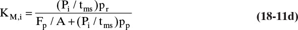
Solving Eq. (18-11b) for yp,i, we obtain
where, after some algebraic rearrangement,
If Eqs. (18-8c) and (18-11c) undergo exactly the same algebraic steps used for flash distillation [from Eqs. (2-36) to (2-37)], the resulting equation for yr,i (equivalent to xi in flash) is
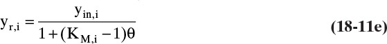
and the summation equation ∑ yr,i = 1.0, (equivalent to ∑ xi = 1.0 in flash) is
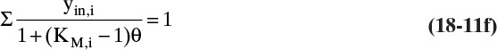
which is essentially same as flash distillation Eq. (2-40a) (see Problem 18.C5). If we multiply Eq. (18-11e) by KM,i and note yp,i = KM,iyr,i we obtain an equation equivalent to ∑ yi = 1.0 in flash.

Thus, KM,i is the membrane equivalent of the equilibrium Ki value in flash distillation.
In a simulation problem all Pi and yi,in values, tms, pr, pp, Fin, and area A are known, but permeate volumetric flow rate Fp or equivalently cut θ are unknown. This problem is equivalent to the classic multicomponent flash distillation problem in which V/F is unknown. In flash distillation the best convergence scheme was the Rachford-Rice equation derived by starting with ∑ yi – ∑ xi = 0. For membranes the equivalent convergence method, ∑yp,i – ∑yr,i = 0, also appears to be best. The procedure mimics the procedure used for flash distillation:
1. Pick a value of θ between 0.0 and 1.0.
2. Calculate Fp = θ Fin.
3. Calculate each KM,i from Eq. (18-11d).
4. Calculate ∑yp,i from Eq. (18-11h) and ∑yr,i from Eq. (18-11f).
5. Calculate Check = [∑yp,i – ∑yr,i].
6. If Check ≠ 0, pick a new value of θ and repeat. A convenient method for obtaining convergence is to use Goal Seek in Excel.
This procedure is illustrated in Example 18-3. Although shown only for gas permeation, this approach can be used with other perfectly mixed membrane separators.
EXAMPLE 18-3. Multicomponent, perfectly mixed gas permeation
A perfectly mixed gas permeation unit is separating a mixture that is 20.0 mol% carbon dioxide, 5.0 mol% oxygen, and 75.0 mol% nitrogen using a poly(dimethylsiloxane) membrane at 25.0°C. Feed flow rate Fin = 20,000 cm3 (STP)/s. Membrane thickness is 1.0 mil (0.00254 cm). Feed pressure is 3.0 atm, and permeate pressure is 0.40 atm. Membrane area = 150.0 m2. Find cut θ = Fp/Fin and the outlet mole fractions of permeate and retentate.
Solution
Permeabilities (Table 18-2) are PCO2 = 3240.0 × 10–10, PO2 = 605 × 10–10, PN2 = 300.0 × 10⁻¹⁰, all in [cm3(STP)cm/(cm2 s cm Hg)]. So that we do not forget, change the units of pressures: pr = 3.0 atm (76.0 cm Hg/atm) = 228 cm Hg, pp = 0.40 atm = 30.4 cm Hg.
The KM,i values can be calculated from Eq. (18-11d). For example, for carbon dioxide

and similarly for oxygen and nitrogen. To use these terms in a trial-and-error procedure, we need to start with a value for Fp or equivalently θ (Fp = θ Fin).
If we arbitrarily pick θ = 0.100 (Fp = 2000.0 cm3 (STP)/s),

KM,O2 = 2.63956, and KM,N2 = 1.59119. In flash distillation some Ki values had to be greater than 1 and some less than 1. This is also true of KM,i values. From Eqs. (18-11f) and (18-11h) calculated value of ∑yp,i – ∑yr,i = 1.1174 > 0.0. A higher value of θ is required. This problem was set up in a spreadsheet, and Goal Seek was used for convergence of θ.
The final results obtained were: θ = 0.29364, Fp = 5873 cm3 (STP)/s, ∑yp,i – ∑yr,i = 4.13 × 10⁻⁷, ∑yr,i = 0.99999988, yp,CO2 = 0.41415, yp,N2 = 0.53011, yp,O2 = 0.05574, yr,CO2 = 0.11097, yr,O2 = 0.04761, yr,N2 = 0.8414, KM,CO2 = 3.7320, KM,O2 = 1.1706, and KM,N2 = 0.6300.
Converging ∑yp,i – ∑yr,i = 0.0 works for any first guess of θ in physically reasonable range from 0.0 to 1.0. Converging on ∑yp,i = 1.0 or ∑yr,i = 1.0 does not always converge on the correct answer.
Permeate is not very pure. Although nitrogen has the lowest permeability, there is still more nitrogen than carbon dioxide in permeate. This occurs because the large amount of nitrogen in feed produces a large driving force to push nitrogen through the membrane. Retentate is significantly purer than feed. To obtain a relatively pure nitrogen stream in retentate with this feed, we can increase cut and retentate pressures (see Problem 18.D12); however, a better approach is to use a membrane with higher selectivity.
In a design problem all Pi values, tms, pr, pp, Fin, yi,in, and permeate volumetric flow rate Fp (or θ) are known, but area A is unknown. The easiest method to find the area required for a multicomponent permeator appears to be to follow same procedure as in Example 18-3, except guess value of A instead of θ. Converging ∑yp,i – ∑yr,i = 0.0 appears to work for a very broad range of estimates of A as long as A > 0.0.
To be sure you know how to do multicomponent permeation problems, set up your own spreadsheet, and solve at least one of the following: Problem 18.D12, 18.D18, 18.D27, or 18.H1. Geankoplis (2003) solves multicomponent permeator systems using a different method, but the results are identical (see Problem 18.H1).
18.3.4 Effect of Holes in Membrane
Since we have not allowed for any other mechanism for flow from high to low pressure, our calculations assume the membrane is perfect and has no pinholes. Pinholes allow convective flow of high-pressure fluid into the permeate. Since fluid that flows through a pinhole has not gone through the membrane, its mole fraction is yw. As a result, it contaminates the permeate product.
We can do an approximate calculation of flow rate through a pinhole and estimate the magnitude of the effect of the pinholes. Assume the hole is a tube of radius R and length L = tms, flow is laminar, change in potential energy (ρgΔz) is negligible, there are no entrance or exit effects, and flow is at steady state. The equation for volumetric flow rate Q is (Bird et al., 2006).
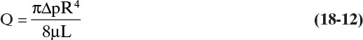
where µ is viscosity, and Δp = pr – pp. Although Eq. (18-12) is not strictly applicable because there are certainly entrance and exit effects, it will give a reasonable estimate of magnitude of the effect of the holes on purity.
The membrane system studied in Example 18-1 is separating a feed that is 95.0 mol% carbon dioxide and 5.0 mol% nitrogen at 25.0°C in a perfectly mixed gas permeation module. Our goal is to obtain a high purity CO2 product with yp,CO2 ≥ 0.995. Module has 50.0 m2 of membrane and is operated with a retentate pressure of 5.5 atm and a permeate pressure of 1.01 atm. Membrane thickness is tms = 1.0 × 10⁻⁴ cm. Cut θ = 0.20.
A. Find yp,CO2, yr,CO2 = yr,out,CO2, JCO2, Fm,p (in mol/min), and Fm,in (in mol/min) for a perfect membrane.
B. Assume there is one pinhole of diameter 10.0 µm per m2. Calculate the convective flow rate through the pinhole.
C. For the same Fm,in as part a and the same pinhole as part b, find the total permeate flow rate, yp,CO2, and yr,out,CO2.
D. Repeat parts c and d if the pinholes are 1.0 µm in diameter but with one hole/cm2.
Data: From Example 18-1: PCO2 = 75 and PN2 = 4.43, both cm3 (STP)cm/[cm2s cm Hg] × 10–10. Then αCO2–N2 = (75.0 × 10⁻¹⁰)/(4.43 × 10–10) = 16.9. Pressure ratio pr/pp = 5.5/1.01 = 5.446. Δp = 4.49 atm. For ideal gases, ρm,CO2/ρm,N2 = 1.0 and ρm,CO2 = 1 mol/22.4 L(STP).
Data: µCO2 = 0.0154 cp = 0.000154 g/(cm s), µN2 = 0.0177 cp = 0.000177 g/(cm s) (source: www.lmnoeng.com/Flow/GasViscosity.php).
Solution Part A: Any method discussed earlier (including the method for multicomponent feeds) can be used. Results: Fm,in = 159.439 mol/min, Fm,p = 31.888 mol/min, yp,CO2 = 0.9953, yr,CO2 = 0.9387. We have met our purity requirement if there are no holes.
Solution Part B: Since the product is almost pure CO2, use CO2 viscosity. Equation (18-12) becomes
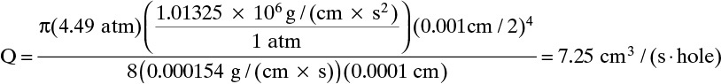
Q is at outlet pressure and temperature. To convert to STP (25.0°C and 1.0 atm), Q (STP) = Q(Tr,pr) × (pr/1.0 atm) × (298.15 K/Tr) = 7.25 × (1.01/1.0) × (298.15/298.15) = 7.325 cm3(STP)/(s·hole)

Since we assumed one hole per m2, convective flux through the holes is 0.0196 mol/(min m2). With 50.0 m2, this is 0.981 mol/min. For a well-mixed module, concentration of this gas is yr,CO2 = 0.93868.
Solution Part C: With one hole/m2, the total permeate product flow rate = 31.88 + 0.981 = 32.86 mol/min.
CO2: yCO2,product = [31.88yp,memb + 0.981yr]/32.86 = [31.88(0.9953) + 0.981(0.93868)]/32.86 = 0.9936.
We no longer meet our purity requirement.
Solution Part D: Values of Q and Qmol are multiplied by 10–4; however, with one hole per cm2, flux per m2 is Qmol × 104, net flux is the same as previously, and the values are same as in part c.
Comments: If high purity is required, membrane flaws can prevent gas permeation from achieving desired permeate purity. For a membrane with an active layer 1 micron thick, one 10-micron pinhole per m2 is good quality control, but it may not be good enough for high-purity products. If a significantly thicker separating layer is used it is easier to produce a product with no holes, but flux is reduced. A different approach that is used commercially is to cast the membrane and then cast a thin layer of silicone rubber over entire membrane (Henis and Tripodi, 1983). Silicone rubber fills holes preventing convective flow and because it has a high permeability, adding a thin layer does not decrease membrane flux significantly.
18.4 Reverse Osmosis (RO)
There is a global water crisis. Only one chemical—water—was named in the National Academy of Engineering’s Grand Challenges. Earth is blessed with abundant water, but many places have a shortage of clean water. The grand challenge is to “provide access to clean water” (National Academy Engineering, 2015).
RO is the most commonly used process to purify and desalinate water (Reisch, 2007). RO is an integral part of industrial water management plans to reach zero-liquid discharge goals (Kucera, 2010). In RO liquid water is forced under pressure through a nonporous membrane in the opposite direction of osmosis (osmosis is defined shortly). Most salts and uncharged molecules are retained by the membrane. Thus, permeate is much purer water and retentate becomes significantly more concentrated. A typical seawater desalination system recovers between 50% and 55% of feed water as potable water.
Commonly used membranes shown in Figure 18-3 are: 1) a blend of cellulose acetate and cellulose triacetate, 2) aromatic polyamides (aramids), and 3) cross-linked aromatic polyamides (Eykamp, 1997). Currently, the best membranes are thin-film interfacial composite membranes (Baker, 2004; Uemura and Henmi, 2008). Both hollow-fiber and spiral-wound modules are used for RO (Figure 18-1), but about 85% of applications use spiral-wound membranes (Baker, 2004). Spiral-wound membranes do not clog as easily as hollow fibers; thus, less pretreatment is needed.
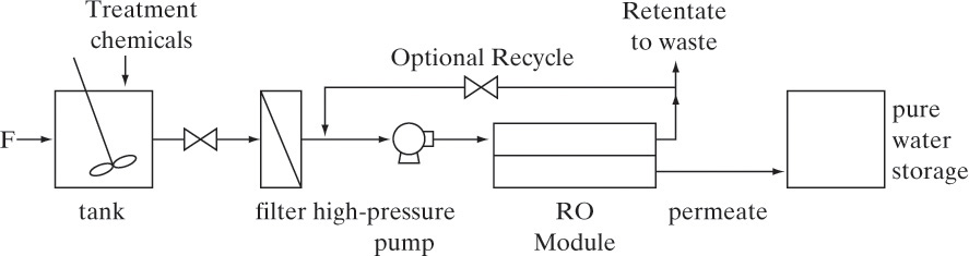
Feed to an RO system usually requires pretreatment to remove particulates that would clog the membrane. If there are ions or solutes in solution that have limited solubility, design must include a solubility calculation to determine if they will precipitate onto the membrane when retentate is concentrated. If precipitation is likely, these ions or solutes must either be removed or made more soluble to prevent them from precipitating. A schematic of a simple RO system including the most important auxiliary equipment is shown in Figure 18-8. In practice, large-scale systems may have hundreds of membrane modules arranged both in series and in parallel (Figure 18-2C) in what is often called a “Christmas-tree” pattern (Baker, 2004). Large-scale systems have pressure exchangers on high-pressure retentate waste lines that recover over 90% of the energy used to pressurize fluid that has not passed through the membrane. More details on equipment are available in Baker et al. (1990), Eykamp (1997), Ho and Sirkar (1992), and Noble and Stern (1995). Kucera (2010) discusses details of operation and maintenance of RO systems.
There are two reasons for studying osmosis in a textbook on separations. First, we need to understand osmosis to design RO systems. The driving force for solvent flux in RO is the difference between the pressure drop across the membrane and the osmotic pressure difference across the membrane (Δp – Δπ). Mass flux of solvent is
In these equations K′solv is solvent (usually water) permeability through the membrane with an effective membrane skin thickness of tms. Pressure drop across the membrane, Δp = pr – pp. Δπ is the difference in osmotic pressure across the membrane.
18.4.1 Analysis of Osmosis
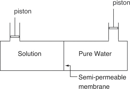
In osmosis solvent flows through a semipermeable membrane (one which passes solvent but does not pass solutes or ions) from less concentrated regions to more concentrated regions. For example, if we have pure water on one side of a semipermeable membrane and a sugar solution on the other side, water will flow into the sugar solution to dilute it. Thus, in Figure 18-9 osmotic flow is from the right (pure water) to the left side (sugar solution). This natural direction of solvent flow equalizes chemical potentials. We can stop or reverse flow by increasing pressure on the sugar solution using the piston shown on the left. Osmotic pressure π is additional pressure required on the concentrated side to stop osmotic flow, assuming the permeate side is pure water that contains no solute.
Osmotic pressure is a thermodynamic property of the solution. Thus, π is a state variable that depends on temperature, pressure, and concentration but does not depend on the membrane as long as the membrane is semipermeable. Osmotic equilibrium requires that chemical potentials of solvent on the two sides of the membrane be equal. Note that solutes are not in equilibrium since they cannot pass through the membrane. Although osmotic pressure can be measured directly, it is usually estimated from other measurements (e.g., Reid, 1966). For an incompressible liquid, osmotic pressure can be estimated from vapor pressure measurements:
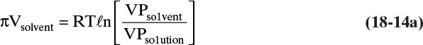
where Vsolvent is partial molar volume of solvent. Another common method is to relate osmotic pressure to freezing-point depression (Reid, 1966).
For dilute systems osmotic pressure is often a linear function of concentration:
As solutions becomes more concentrated, osmotic pressure increases more rapidly than predicted by a linear relationship. For some dilute systems the linear constant can be estimated from the van’t Hoff equation:
Since derivation of the van’t Hoff equation assumes that Raoult’s law is valid, Eq. (18-14d) will be incorrect if solute associates or dissociates even though empirical Eq. (18-14b) may still be accurate. Osmotic pressure, in Pa, for natural waters containing salts can be determined from the following empirical correlations with T in °C and salt concentration Cs in kg/m3 (Geraldes et al., 2005):
Since Cs = xρsolution with ρsolution in kg/m3, Eq. (18-14e) can be written as
However, solution density increases as x increases, which means the equation is no longer linear. Solution densities at 25.0°C (Green and Perry, Table 2-110, Table 2-90, 2008) are: 0.0 wt% NaCl, ρ = 0.997 g/cm3; 1.0 wt% NaCl, ρsolution = 1.00409; and 2.0 wt% NaCl, ρsolution = 1.01112. If we take an average value of ρsolution between x = 0.0 and 0.02 [Eq. (18-14e) is valid up to a concentration Cs = 20.0 kg/m3 or x = 0.0197], we obtain ρavg = 1004.1 kg/m3. If we convert Eq. (18-14g) to π in atm with a′ in atm/weight fraction, the resulting equation is very close to linear in the range of validity.
At T = 25.0°C, a′ = 705.9 atm/weight fraction.
The second reason for studying osmosis is a novel separation system called forward osmosis (FO), which may become important in the future. FO is osmosis but with the addition of chemicals to form a draw solution that is more concentrated than feed water. The result is that pure water is drawn out of the feed water and into the draw solution (Cath et al., 2006; Chung et al., 2012). The process has also been studied for pharmaceutical manufacturing and food processing. There are several attractive features of the process, the main one being that since the FO step is the natural direction of water movement, energy requirements are very low. In addition, the draw solution can be tailored for specific separations such as difficult and high-salinity waters. The major hurdle is one that all mass separating–agent processes (e.g., extraction) must overcome—how to economically recover the pure product from the draw solution and recycle the draw solution. If it is possible to use low-grade, waste energy (e.g., heat from a diesel generator), there may be applications of FO in small desalination plants.
18.4.2 Analysis of Reverse Osmosis
Unfortunately, natural osmotic flow is in the opposite direction to what we normally want to do (produce pure water). In RO we push solvent out of concentrated solution into dilute solution, which requires energy. Because RO is reversing the natural flow direction, RO is inherently a nonequilibrium process. The increase in osmotic pressure as retentate becomes more concentrated also puts a natural limit on recovery of pure solvent by RO. If one tries to recover too much solvent, the retentate becomes very concentrated, the osmotic pressure difference becomes extremely large, and the pressure drop required by Eq. (18-13) for a reasonable flux rate becomes too large for practical operation.
The mass solute flux across the membrane, J′A, can be written as
where K′A is solute permeability, and xw and xp are mass fractions of solute at the membrane wall on the retentate side and in the permeate, respectively. For a membrane with perfect solute retention, K′A = 0. Typical units for terms in Eqs. (18-13) and (18-15) are pressure p and osmotic pressure π in atm, solvent permeance (K′solv/tms) in g/(atm·s·m2), solvent flux J′solv in g/(m2s), salt permeance (K′A/tms) in g/(m2s·mass fraction), and salt flux J′A in g/(m2s). If a large amount of water is removed as product, in addition to increasing osmotic pressure because xr and xw increase, salt flux into permeate also increases.
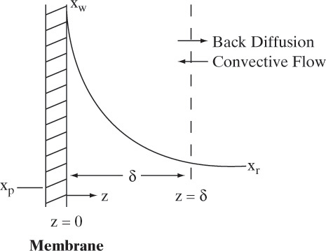
The analysis procedure developed in Section 18.3 for gas permeation is the starting point for analyzing RO. However, RO analysis is more complicated because of 1) osmotic pressure, which is included in Eq. (18-13), and 2) mass transfer rates are much lower in liquid systems. Since mass transfer rates are relatively low, the weight fraction of solute at the membrane wall, xw, is greater than the weight fraction of solute in retentate bulk, xr. Buildup of solute at the membrane surface occurs because solvent movement from the bulk fluid to the membrane carries solute with it. Since solute does not pass through the semipermeable membrane, its concentration builds up at the wall, and it must back diffuse from the wall to the bulk solution. This concentration buildup, concentration polarization, is illustrated in Figure 18-10. Concentration polarization has a major effect on RO and UF separations (see Section 18.5 for UF). Since concentration polarization causes xw > xr, osmotic pressure becomes higher on the retentate side and, following Eq. (18-13), flux declines. Concentration polarization also increases (xw – xp) in Eq. (18-15) and the flux of solute may increase, which is also undesirable. In addition, since concentration polarization increases solute concentration at the wall, precipitation and fouling become more likely.
Solvent flux Eq. (18-13) can be expanded by noting F′solv = F′p(1 – xp) [x is normally mass fraction in RO]:
Osmotic pressure on the retentate side depends on the concentration of solute at the membrane wall. To simplify the analysis, we temporarily assume osmotic pressure is a linear function of weight fraction, Eqs. (18-14c), (18-14g), and (18-14h). Then flux is
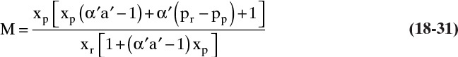
To relate wall concentration to retentate concentration, we define the concentration polarization modulus, M, in terms of weight fractions:
Methods to measure or predict M are developed shortly. Substituting the definition for M in Eq. (18-16b),
Solute flux Eq. (18-15) can also be expanded and written in terms of concentration polarization modulus.
Essentially the same procedure used to develop the RT equation for gas permeators will be used. That is, after assuming that ![]() is not zero and is independent of solvent transfer rate, and that
is not zero and is independent of solvent transfer rate, and that ![]() is independent of solute transfer rate, we will solve Eqs. (18-16c) and (18-18) for F′p, set the two equations equal to each other, and solve for the desired concentration. It is convenient to define membrane selectivity α′ as
is independent of solute transfer rate, we will solve Eqs. (18-16c) and (18-18) for F′p, set the two equations equal to each other, and solve for the desired concentration. It is convenient to define membrane selectivity α′ as
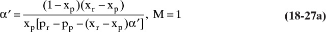
It is easier to solve for xr:

This RT equation represents the transfer rate of solvent and solute through the membrane in mass fraction units. If ![]() , α′ will be infinite, xp will be zero, and xr must be determined from a mass balance. If selectivity is not constant, α′ will depend on xw = Mxr. It will then be convenient to solve for xp as a function of xr.
, α′ will be infinite, xp will be zero, and xr must be determined from a mass balance. If selectivity is not constant, α′ will depend on xw = Mxr. It will then be convenient to solve for xp as a function of xr.
Since RO often operates with high retention of solute and thus very low values of xp, it is useful to simplify RT Eq. (18-20) for small xp. As xp → 0 [(xp α′ a′) << 1.0], Eq. (18-20) becomes
If α′(pr – pp)>>1,
The simplified linear equations are easier to use but are not accurate if (xp α′ a′) is not small enough. Use of Eq. (18-21b) with the mass balance is illustrated in Example 18-6.
18.4.3 RO in Well-Mixed Modules
RT Eq. (18-20) or (18-21) needs to be solved simultaneously with the mass balance. We again assume well-mixed membrane modules. The module is identical to Figure 18-6A, except y terms are replaced by liquid weight fractions. External mass balances (in mass units) are
Solving for xp, we obtain the operating equation

or the alternative
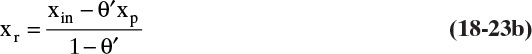
θ′ = F′p/F′in is the cut in mass units. Equation (18-23a) is analogous to Eq. (18-8a) for a well-mixed gas permeator.
In well-mixed modules xr is constant and equal to xout. Thus, Eqs. (18-20), (18-21a), and (18-21b) are valid with xr replaced by xout; however, since there is usually concentration polarization, xw = Mxout, and M must be determined. Once M is known, simultaneous solution of Eqs. (18-20) and (18-23) or of Eqs. (18-21) and (18-23) can be obtained either analytically (see Examples 18-5 and 18-6) or by plotting both equations on a graph of xp vs. xout. Equation (18-23) is a straight line that is identical to the operating line obtained for gas permeation. The RT curve representing Eq. (18-20) or (18-21) can be plotted by calculating values in the same way as in Example 18-2. Note that this curve is below the xp = xout line on a graph of xp vs. xout.
RO data are often reported as the rejection coefficient R.

The rejection coefficient measured with no concentration polarization (M = 1.0) is called the inherent rejection coefficient, Ro, since xout = xr = xw when M = 1.0. The inherent rejection coefficient can be used with concentration polarization if we know the wall concentration or M.

From Eqs. (18-24a) and (18-24b) we can relate R to Ro for any value of M.
If Ro is known and mass fractions xp and xout are specified, the maximum value of M is
If R is known, we can solve Eq. (18-24a) simultaneously with operating Eq. (18-23).
Alternatively, we can solve for xp:

These are very convenient and simple solutions, but R has to be known for the current operating conditions that include concentration polarization effects. Use of these equations is illustrated in Example 18-5.
Solving Eq. (18-20) for selectivity, we obtain
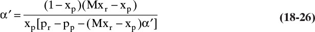
If we do an experiment in a well-mixed membrane module with rapid stirring so that there is no concentration polarization, M = 1.0, Eq. (18-26) simplifies to
Since all terms on the right-hand side are known, we can calculate α′. If linear Eq. (18-21b) is used with Eq. (18-24) for R and we solve for α′, we obtain

Both methods are illustrated in Example 18-5.
EXAMPLE 18-5. Determination of RO membrane properties
We do two experiments to test a new composite membrane. Both experiments are done in a perfectly mixed laboratory system with a retentate pressure of 15.0 atm and a permeate pressure of 1.0 atm. Temperature is 25.0°C. The following data are obtained:
Experiment a. Pure water flux is 1029 L/(m2 day).
Experiment b. With feed weight fraction sodium chloride, xin = 0.00023 (230 ppm weight), rejection coefficient R is measured as 0.993. θ′ = 0.30. You can assume there is no concentration polarization (M = 1.0).
Find water permeance and water-salt selectivity.
Solution
A. Define. Find K′water/tms and α′water–salt.
B. B, C. Explore and plan. Experiment a allows calculation of K′water/tms with xr = xp = 0.0 from Eq. (18-16c). Experiment b allows us to calculate xp and xout from Eqs. (18-25a) and (18-25b). Then, Eq. (18-27a) (with xr = xout and M = 1.0) can be used to find selectivity, α′water–salt.
B. Do it. Experiment a. With xr = xp = 0.0, we can solve Eq. (18-16c) for K′water/tms:
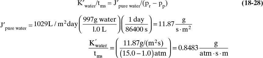
Experiment b. Plugging in numbers to Eqs. (18-25a) and (18-25b) we obtain

In Eqs. (18-26) and (18-27) the term a′ in atm/(mass fraction solute) is the linear coefficient for the effect of concentration on osmotic pressure, Eq. (18-14h). For dilute salts at T = 25.0°C, a′ = 705.9. Selectivity α′ can be determined from Eq. (18-27a):

If we use Eq. (18-27b), the result is
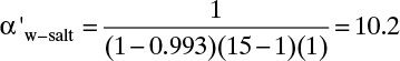
E. Check. For this dilute system we obtain the same results with nonlinear and linearized analyses. Note that the conditions for use of Eq. (18-27b) are satisfied, (xp α′ a′) = (2.293 × 10⁻⁶)(10.2)(705.9) = 0.0165 << 1 and α′(pr – pp) = (10.2)(14) = 142.8 >> 1.
F. Generalize. This example illustrates how to determine parameter values from experiments. Selectivity is used in Example 18-6 to calculate expected behavior of a membrane module when there is no concentration polarization.
1. Pure water flux is often measured and used to find the value of K′solv/tms. This is a preferred method because it is very easy and is quite reproducible. Since flux declines significantly when there is salt present, pure water flux values should never be used as a direct estimate of system’s feed capacity.
2. Rejection data can be used to find value of selectivity, α′w–salt. This selectivity and the permeabilities do not have the same meaning as in gas permeation. Selectivities are defined differently. Permeabilities have different units, and their defining equations have different driving forces.
3. Linearized Eqs. (18-21b) and (18-27a) are convenient, but the test for dilute, (xp α′ a′) << 1.0 requires either a very low value of xp or a much lower value for a′ than salts. Solutes such as sugars have significantly lower values of a′ than NaCl.
By manipulating Eqs. (18-21b) and (18-24), we can find a relationship between retention, R, at one set of conditions and R at another set of conditions for dilute, well-mixed systems. A convenient base case (Case A) condition is an experiment with no concentration polarization (MCase A = 1.0 and RCase A = Ro). Substitute Eq. (18-21b) into the definition of R, Eq. (18-24), for both Cases A and B. Solve for 1.0 – R in both equations and then divide Case B equation by Case A equation. The ratio is

This equation is valid for linearized RT equation (18-21b), which requires
Equation (18-29a) allows calculation of R for different values of M and (pr – pp) for the same membrane if R is known at Case A conditions and the inequalities in Eq. (18-29b) are satisfied. Unfortunately, the restrictions in Eq. (18-29b) are quite severe for salts because a′ is large.
If pressure difference (pr – pp) is the same in the two runs, then
Remarkably, Eq. (18-29c) can be obtained exactly without linearization (except for osmotic pressure) by starting with Eq. (18-20) and requiring constant (pr – pp) and constant permeate mass fraction xp. Since Eq. (18-20) required that osmotic pressure be a linear function of weight fraction (a term), Eq. (18-29c) is restricted to relatively low concentrations [less than 2.0% by weight salt according to Eq. (18-14h)], but this restriction is much less confining than Eq. (18-29b).
EXAMPLE 18-6. RO without concentration polarization
We continue testing the new composite membrane from Example 18-5 in a perfectly mixed membrane system but now with retentate pressure of 10.0 atm and permeate pressure of 1.0 atm. Find the outlet weight fractions of the permeate and retentate streams. There is a very high mass transfer coefficient, and M = 1.0.
a. θ′ = 0.02 (ratio mass flow rates), and feed is 0.04 wt% sodium chloride.
b. θ′ = 0.40, and feed is 1.0 wt% sodium chloride.
Solution
A. Define. Find xp and xout for parts a and b.
B, C. Explore and plan. RT Eq. (18-20) and operating Eq. (18-23b) can be solved simultaneously to find xp and xout. Since change in operating conditions affects only the operating equation, the RT equation is the same for both parts a and b.
D. Do it. If we use Eq. (18-23b) to substitute for xr in Eq. (18-20), we obtain

With θ′ = 0.02, xin = 0.0004 α′ = 10.2, a′ = 705.9, pp = 1.0, pr = 10.0, and M = 1.0, this is a quadratic equation in xp. The equation can be solved by the quadratic formula or with an Excel spreadsheet using Goal Seek or Solver. Once xp is known, xr can be found from Eq. (18-23b).
Part a. θ′ = 0.02, xin = 0.0004, and M = 1.0. Spreadsheet results: xp = 4.548 × 10⁻⁶, xr = 0.000408, R = 0.989.
Part b. θ′ = 0.40, xin = 0.010, and M = 1.0. Spreadsheet results: xp = 0.002721, xr = 0.01485, R = 0.8168.
E. Check. Linearization should give similar results for part a because the very low permeate weight fraction is close to satisfying the restriction in Eq. (18-29b) for using linear forms Eqs. (18-21a) and (18-21b), [(xp α′ a′) = 0.0327 << 1.0]. Solving Eq. (18-21b) simultaneously with operating Eq. (18-23b) we obtain

The result from Eq. (18-30b) is xp = 4.445 × 10⁻⁶, and from Eq. (18-23b), xr = 0.000408. The retentate is exact, and the more sensitive permeate weight fraction is off by 2.3%.
For part b the linear equation results are: xp = 1.80 × 10⁻⁴, and from Eq. (18-23b), xr = 0.0165, which are not very accurate because (xp α′ a′) = 19.6 is too high for linearization.
F. Generalize. This example showed that at low concentrations the linearization procedure used for Eqs. (18-21a), (18-21b), and (18-27b) is valid, but as feed mass fraction increases, linearization becomes less valid.
18.4.4 Mass Transfer Analysis of Concentration Polarization
Once values for α′ are known, experiments can be done with conditions in which concentration polarization is expected. Solve Eq. (18-20) for M.
Since all terms on the right-hand side are known or measured, M can be calculated from experimental data.
However, estimation of M will allow us to avoid doing expensive and time-consuming experiments. Concentration polarization was shown schematically in Figure 18-9. This figure applies to the simplest situation–steady-state, one-dimensional back diffusion of one solute into a bulk retentate stream with a perfectly rejecting membrane (R = 1.0). (If rejection is not almost complete, more detailed theories are required [e.g., Ho and Sirkar, 1992; Noble and Stern, 1995; Wankat, 1990].) The differential mass balance for this simple situation using a Fickian analysis is (Problem 18.C3):

where D is Fickian solute diffusivity in liquid solution in m2/s, and ρsolv is in g/m3. Boundary conditions are solute concentration equals solute wall concentration at z = 0:
and concentration becomes bulk concentration xr when z is greater than or equal to boundary layer thickness δ.
The value of δ depends on operating conditions (geometry, velocity, T). Defining the mass transfer coefficient in the usual form,
the solution is
Since δ depends on operating conditions, mass transfer coefficient k also depends on operating conditions. k has units of m/s. If there are multiple solutes, a Maxwell-Stefan analysis (Section 15.7) is recommended.
This short, and overly simplified, development is useful to determine what affects concentration polarization. If solvent flux J′solv increases, M increases. If mass transfer coefficient k increases, concentration polarization decreases. Increasing diffusivity increases k. Thus, operating at a higher temperature decreases M, although there are obvious limits based on membrane thermal stability and thermal stability of solutes (e.g., most proteins are not thermally stable). Decreasing boundary layer thickness δ by promoting turbulence or operating at very high shear rates in thin channels or narrow tubes also increases k.
The quantitative use of Eq. (18-34a) requires either experimentally determined values of mass transfer coefficient k or a correlation for k (which is ultimately based on experimental data). If experimental data are available that allow calculation of M from Eq. (18-31), then k can be determined by solving Eq. (18-34a) for k.
A large number of mass transfer correlations are available for a variety of geometries and flow conditions (Wankat and Knaebel, 2008). Five that are useful for membrane separators are correlations for turbulent flow in tubes, for turbulent flow in spiral wound membrane modules, for laminar flow in tubes and between parallel plates, and for well-mixed tanks (Blatt et al., 1970; Schock and Miquel, 1987; Wankat, 1990; Wankat and Knaebel, 2008). For turbulent flow in tubes the mass transfer coefficient can be estimated from

where Sh is the Sherwood number, and the Reynolds number, Re, and Schmidt number, Sc, are defined as
d is tube diameter, and ub is bulk velocity in the tube. Fully developed turbulent flow certainly occurs for Re > 20,000, and usually appears in UF devices for Re > 2000.0.
Spiral-wound membranes (Figure 18-1C) are most commonly used for water treatment. Spacers in the feed channel are designed to promote turbulence and increase mass transfer rates. Schock and Miquel (1987) experimentally determined a mass transfer correlation for typical spiral-wound modules.

Here Ds is salt diffusivity, and Re is defined by Eq. (18-35b) with d = the height of feed channel. This equation is similar to Eq. (18-35a) but predicts a higher mass transfer coefficient because of the turbulence-promoting spacers.
For laminar flow in tubes of length L and radius R with a bulk velocity ub, the average mass transfer coefficient is
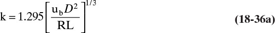
For laminar flow between parallel plates with a spacing of 2 h, the average mass transfer coefficient is
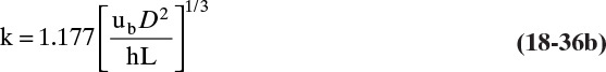
For flat membranes in a well-stirred turbulent tank, the mass transfer coefficient can be estimated from

In Eqs. (18-37a) and (18-37b) k is in cm/s, ω is stirrer speed in radians/s, dtank is tank diameter in cm, D is diffusivity in cm2/s, and kinematic viscosity ν = µ/ρ is in cm2/s. Stirred tanks are a convenient laboratory configuration.
EXAMPLE 18-7. RO with concentration polarization
We continue testing the new composite membrane explored in Examples 18-5 and 18-6. An additional experiment is done at 25.0°C with a retentate pressure of 15.0 atm and a permeate pressure of 1.0 atm. In addition to data reported in Example 18-5, the following new data are obtained:
Experiment c. Experiments are done in a baffled stirred-tank system with a 35.0 cm–diameter tank. We expect that Eq. (18-37a) is valid, except coefficient 0.04433 has to be adjusted. Stirrer is operated at 900.0 rpm. Inlet solution is 0.5 wt% sodium chloride. The measured weight fractions are xp = 8.252 × 10⁻⁵, and xout = 0.006229.
Based on these experiments determine the value for the constant in correlation for mass transfer in turbulent stirred tanks Eq. (18-37a).
Solution
A, B, and C. Define, Explore, and Plan. Calculate polarization modulus M from Eq. (18-31), J′solv from Eq. (18-16c), and mass transfer coefficient k from Eq. (18-34b), and solve Eq. (18-37a) for the constant.
D. Do it. Experiment c. Since xp and xout were measured, and α′ = 10.2, a′ = 705.9, pr, and pp are all known, M can be determined from a straightforward plug-and-chug calculation in Eq. (18-31).
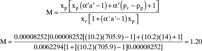
Solvent flux can be determined from Eq. (18-16c) using K′solv/tms = 0.8483 determined in Example 18-5. Because xr = xout for a well-mixed tank,
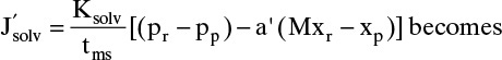
J′solv = 0.8483{(15.0 – 1.0) – 705.9[(1.20)(0.006229) – 0.00008252]} = 7.45 g/(m2·s)
Note that this is about 65.0% of pure water flux (11.87) because driving force is reduced by osmotic pressure difference. From Eq. (18-34b)

Solving for the constant in Eq. (18-37a), we obtain

The density of solution for dilute salt solutions was given immediately after Eq. (18-14g). Linearly interpolating to xr = 0.006229, we find ρsolution = 1001.4 kg/m3. Since the solution is quite dilute, the properties of water will be used for other properties.
ρ = 1.0014g / cm3, μ = 1.0 cp = 0.01 poise = 0.01 g / (cm · s)ν, = μ / ρ = 0.01 / 1.0014
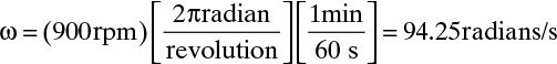
The diffusivity of NaCl in water at 25.0°C is 1.53 × 10⁻⁵ cm2/s.
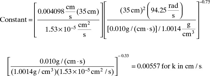
E. Check. It is not unusual to have a general mass transfer correlation differ from experiment by this much. We will use the measured value of the constant in Example 18-8.
F. Generalization. This example illustrates how we can use experimental data and fine tune mass transfer correlations by adjusting the constants.
Experiment c required a number of steps to eventually find mass transfer coefficient k. This is invariably the case, since k is not a directly measured variable but depends on interpretation of data using a model. Knowing the value of k, we have a single data point to compare to correlation Eq. (18-37a). They disagreed. You may be tempted to use the correlation and ignore the data point. However, mass transfer correlations are not very accurate. They usually predict trends well (such as the effect of Reynolds and Schmidt numbers), but absolute values predicted can be significantly off. If it is reliable, a single data point can be used to adjust the constant in the correlation for application to this particular system. If more data were available, we could check the entire correlation.
EXAMPLE 18-8. Prediction of RO performance with concentration polarization
Predict values of xp, xout, and J′solv if a 1.0 wt% sodium chloride in water solution is separated by the membrane studied in Examples 18-5 to 18-7 in a stirred tank that is geometrically similar to the one in Example 18-7, except the tank is 40.0 cm in diameter, and the stirrer speed is 500.0 rpm. Retentate pressure is 20.0 atm, and permeate pressure is 1.0 atm. Operate at a cut θ′ = 0.40 and at 25.0°C.
Solution
A, B, and C. Define, Explore, and Plan. We can now calculate mass transfer coefficient k using D, ρ, µ, and the coefficient = 0.00557 from experiment c and Example 18-7.
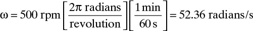
From Eq. (18-37a) with the modified constant,
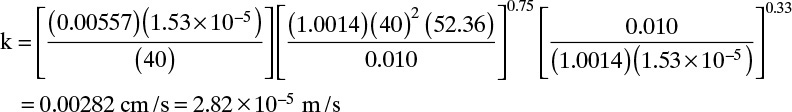
At this point we can proceed to use a permeation analysis. Unfortunately, the feed is too concentrated to use the simpler linearized analysis, so we must use Eq. (18-30a).
Parameter values: (pr – pp) = 19, θ′ = 0.40, xin = 0.01, a′ = 820.0, K′solv/tms = 0.8483 (g/atm s m2), k = 2.82 × 10⁻⁵ m/s (to have consistent units, k has to be in m/s.)
With a guessed value, Mguess, we proceed as follows:
1. Solve Eq. (18-30a) by guessing xp, calculating the values of the right- and left-hand sides of Eq. (18-30a), and using Goal Seek to converge on the xp value that makes RHS = LHS. One could also use the solution of a quadratic equation [similar to Eq. (18-10e)] to solve for xp.
2. Once xp is known xr can be found from Eq. (18-23b).
3. Find J′solv from Eq. (18-16c): J′solv = (K′solv/tms)[(pr – pp) – a′(Mxr – xp)].
4. Calculate M from Eq. (18-34a): Mcalc = exp[(J′solv/ρsolv)/k].
5. If |Mcalc – Mguess| < ε, then the calculation is correct. If not, use a new value of Mguess and repeat. ε = 0.001 is reasonable. A damped substitution of Mnew = Mold + (df) × (Mcalc – Mold) with a damping factor df = 1/2 worked well for convergence of M.
D. Calculations. A spreadsheet was set up to calculate the steps in order. The converged solution was xp = 0.0003384, xr = 0.01644, R = 0.9794, J′solv = 4.689, and M = 1.18145.
E. Check. Note that xr is within the linear range for estimating osmotic pressure π. The results obtained are consistent with what we expect. This is a helpful and quick check but does not guarantee there are no errors.
1. The prediction of performance was trial and error because the unknown variables were needed to calculate other unknowns that were needed to calculate the first unknown. This circle is broken by guessing a variable, doing the calculation, and then checking the guess. Convergence was rapid. In more concentrated systems or with less vigorous stirring with much larger M and larger π values (which may be nonlinear functions of weight fraction), convergence can be slower.
2. RO is commonly used to produce ultrapure water in the electronics and pharmaceutical industries. In these applications Ro is close to 1.0, and xin is often in the ppm range. These systems have little concentration polarization (M ∼ 1.0) and produce very pure permeate.
3. All of these calculations assume an undamaged membrane with no holes. Even a tiny pinprick can cause a large increase in xp (see Problem 18.D22). Liquid passes through a hole as convective flow at a salt concentration of xw. This flux is quite large because of the large pressure drop. In addition, undesired large molecules can also pass through holes in the membrane. Performance of RO systems needs to be monitored continuously, and damaged membranes need to be plugged or replaced.
4. Membrane life depends on membrane material and operating conditions. Membrane replacement costs should be included in operating expenses.
5. If a limiting case does not agree with an independent calculation, then there must be an error in either the original calculation, the method to produce the limiting case, or the independent calculation. If the limiting case agrees with an independent calculation (as it does for this problem for M = 1.0), we have not proved that the calculation for M > 1.0 is correct. As the number of limiting cases that agree with independent calculations increase, our confidence in the general solution increases.
6. If the tanks were not geometrically similar, the constant in mass transfer correlation, Eq. (18-37a), is probably different for the two tanks. Geometric similarity allows one to scale-up.
18.5 Ultrafiltration (UF)
UF is another membrane separation method used to purify liquids. UF is commonly used for recovery of proteins and in food and pharmaceutical applications. It is useful for separating permanent emulsions since oil droplets will not pass through the membrane. UF is used for removal of fine colloidal particles and for recovery of dyes from wastewater. In many applications such as whey processing UF and RO are used in series. Valuable proteins are recovered by UF, and UF permeate is RO feed. RO concentrates remaining sugars and salts by removing water. Concentrated permeate can then be fermented to produce ethanol, lactic acid, and other products.
Equipment for UF systems often looks very similar to RO systems, although they operate at lower pressures. However, this similarity does not extend to the molecular level. Remember that RO membranes are nonporous and separate based on a solution-diffusion mechanism. UF membranes are porous and separate based on size exclusion. Large molecules are excluded from pores in the thin membrane skin, and thus, large molecules are retained in retentate. Small molecules fit into pores and pass through to permeate. Since there is usually a distribution of pore sizes, molecules within the range of pore sizes partially permeate and are partially retained. In a somewhat oversimplified picture, UF is crossflow filtration at the molecular level.
Because of their porous structures, UF membranes have significantly higher fluxes than RO membranes. Thus, concentration polarization is usually worse in UF than in RO because there is a much greater solvent flow from bulk fluid through the wall. Concentration polarization can cause membrane fouling, which not only decreases flux but also can drastically decrease membrane life. Hydrophilic membranes tend to foul less rapidly but have shorter lives than more stable hydrophobic membranes. The best membrane depends on the operating conditions. Cellulose acetate (Figure 18-3) membranes were the first commercial membranes and are still used where their low level of interaction with proteins is more important than their relatively short life. Polymeric membranes are used where more basic conditions are encountered. The most common polymeric membrane is polysulfone (Figure 18-3). Membranes are tailor-made to sieve molecules in different size ranges depending on the purpose of the separation (Figure 18-11). Nominal molecular weight exclusion (shown by x in Figure 18-11) is often reported by manufacturers, but it is not nearly as useful as a complete retention curve.
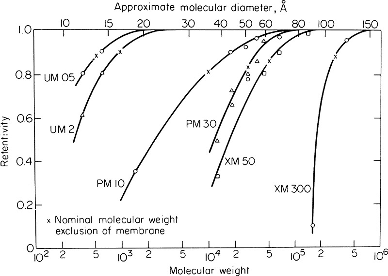
FIGURE 18-11. Solute retention on Amicon Diaflo membranes (Porter, 1997), reprinted with permission from P. A. Schweitzer (Ed.), Handbook of Separation Techniques for Chemical Engineers, 3rd ed., (1997), copyright 1997, McGraw-Hill.
With low concentration polarization UF can be analyzed by procedures used for RO; thus, Eqs. (18-12) and (18-16) are valid. However, in UF retained molecules are often very large, and osmotic pressure difference is very low. For most UF applications osmotic pressure difference can be ignored, which simplifies solvent flux equations. In mass units solvent flux is
where F′p is mass transfer rate of permeate (e.g., kg/s), and xp is weight fraction of solute in permeate. As we will see, ignoring the osmotic pressure difference is a more important simplification than it looks at first.
For sieve-type membranes if a pore does not exclude solute, it will pass solute at the wall weight fraction, xw = Mxr. In sieve-type membranes inherent rejection Ro (M = 1.0) can be interpreted as fraction of flux carried by pores, which exclude solute. Then 1.0 – Ro is fraction of flux carried by pores that do not exclude solute. Ideally, Ro is independent of (pr – pp), and by definition Ro is independent of M.
The permeate weight fraction, xp, is then
This equation can also be solved for retentate weight fraction:
Equations (18-39) and (18-40) are the RT equations for UF. They are particularly simple because inherent rejection Ro is based on experimental data. The retention definition for UF is microscopic, which is different than the macroscopic definition used for RO [Eq. (18-24)]. RT equations for UF depend only on inherent solute rejection and M. For a perfectly mixed membrane module we assume that xr = xout. Then either Eq. (18-39) or (18-40) written in terms of xout can be solved simultaneously with mass balances, Eqs. (18-22) or operating Eq. (18-23). Equations (18-23) and (18-39) or (18-40) can also be solved simultaneously to obtain

Note the differences between UF Eqs. (18-39) to (18-41) and RO Eqs. (18-25) and (18-26). Since Ro in UF is approximately constant, the polarization modulus appears in Eqs. (18-39) to (18-41) from the concentration of material transferred through pores. In RO the value of R depends on both M and (pr – pp), and M does not appear explicitly in Eqs. (18-25) and (18-26).
Experimental results with low-concentration feeds or under conditions where M is close to 1.0 are in good agreement with theoretical predictions. However, when wall concentration becomes high, solvent flux Jsolv often cannot be controlled by adjusting the pressure difference. Thus, Eq. (18-38) no longer holds! Some other phenomenon must be controlling solvent flux. Careful examination of membrane surfaces after these experiments shows a gellike layer covering the membrane. This gel layer alters the flux-pressure drop relationship and controls solvent flow rate.
The effect of gel formation at the wall can be studied using the diffusion equation. Return to Figure 18-10. We implicitly assumed that wall concentration was a variable that could increase without bound. In gelling systems once wall concentration equals the gel concentration, xg, concentration at the wall becomes constant at xw = xg. As additional solute builds up at the wall, the gel concentration is unchanged, but the gel layer thickness increases; thus, xw becomes a constant set by solute gelling behavior. This is illustrated in Figure 18-12. The values of xg vary from less than 1 wt% for polysaccharides to 50 vol% for polymer latex suspensions (Blatt et al., 1970).
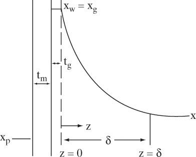
To analyze gelling systems we can again use Eq. (18-32a) when R = 1.0. (Once a gel forms it is usually quite immobile, and 100% retention is reasonable.) With the coordinate system redefined as in Figure 18-12, boundary conditions are the same as Eqs. (18-32b) and (18-32c). The solution has same form as in Eq. (18-34); however, since xw and xr are fixed, solvent flux is the variable. If we solve for solvent flux, we obtain
The consequence of this equation is that once a gel has formed solvent flux is set by rate of back diffusion of solute. We no longer control solvent flux!
What happens if we increase pressure drop across the membrane for a system with a gel present? Solvent flux temporarily increases, but more solute is carried to the membrane than can be removed by back diffusion. The extra solute is deposited on the gel layer, which increases the gel layer’s thickness. This increases flow resistance, which reduce flux through the membrane until the steady-state solvent flux given in Eq. (18-42) is again obtained. This effect is usually not reversible. Reduction of pressure results in a flow rate less than that predicted by Eq. (18-42) because the thicker gel layer remains on the membrane. A gel layer can often be removed by shutting down the system and back flushing (running pure solvent at a higher pressure on the permeate side) or by mechanical scrubbing of the membrane. Unfortunately, if gel fouls the membrane, it may be very difficult to return the membrane to its original flux behavior. Fouling-resistant membranes should be used under gelling conditions.
Designers have some control since decreasing boundary layer thickness, δ, with thin channels or turbulence increases mass transfer coefficient k and hence flux. To a limited extent D can be increased by raising temperature. Effect of these variables on mass transfer coefficients can be explored using correlation Eqs. (18-35) to (18-37). If fouling is severe after gel formation, it may be necessary to operate so that gels never form: xw = Mxr < xg at all times. This can be done by operating under conditions that reduce M (high values of k) and keeping xr low (low feed concentrations and low cuts). The feed-and-bleed system in Figure 18-2 is frequently used because very high velocities and hence larger k can be achieved. When a gel does not form solvent flux in UF is controlled by Eqs. (18-38), the concentration polarization modulus can be calculated from Eq. (18-34), and solution is straightforward. When feed-and-bleed systems are used to concentrate solute, the purpose is to retain all solute (often a polymer), and operation is often at the highest flux rate, which is given by Eq. (18-42) when gel just starts to form. Foley (2016) illustrates solution methods for these steady-state systems.
Most feeds processed by UF contain a number of different solutes. How should we analyze these separations? An almost overwhelming temptation is to study each solute individually and then assume that superposition is valid. That is, we assume that each solute in a mixture behaves in the same way it does alone. After all, this is what we did for gas permeation and RO. Thus, we would predict that large molecules will be retained and small molecules will pass through the membrane. If no gel forms, this behavior is often observed; however, if a gel forms, the gel is usually much tighter (less porous) than the membrane, and the gel layer usually captures small molecules. Thus, separation behaviors with and without gels can be quite different. If the purpose of UF is to separate large and small molecules, then we must operate under conditions where a gel will not form. Gel formation and fouling have prevented UF from achieving its full potential because they often limit both separation and flux.
Although fluxes are lower, RO membranes can also cause gelling and foul if they are operated with feeds that can gel or that contain particulates. To prevent fouling it is common to put an UF system before a RO system. Then the UF system removes particulates and large molecules that could foul the RO membrane. This procedure is followed in whey processing in which UF retains proteins and RO retains sugars and salts.
EXAMPLE 18-9. UF with gel formation
We are ultrafiltering latex particles, which are known to form a gel when xw = xg = 0.5. The well-mixed system is operated with permeate pressure of 1.0 bar and retentate pressure of 4.5 bar. We do a series of experiments with different inlet concentrations with a cut θ′ of 1/3. Permeate weight fraction is zero for all experiments. Experiments show gelling occurs when xin = 0.1466, and measured flux is J′ = 51.93 g/(m2⋅s). Predict the solvent flux that will result in a gel layer for inlet weight fraction xin = 0.20.
Solution
A. Define. Find ![]() that results in xw = xg = 0.5 when xin = 0.20, θ′ = 1/3, pp = 1.0 bar, and pr = 4.5 bar.
that results in xw = xg = 0.5 when xin = 0.20, θ′ = 1/3, pp = 1.0 bar, and pr = 4.5 bar.
B, C. Explore and plan. Use a mass balance to determine xr = xout for xin = 0.1466 and Eq. (18-45) to determine k using measured flux at this inlet weight fraction. Then for xin = 0.20 find xr = xout (since xp is reliably zero, we can assume it remains zero for xin = 0.20). Use Eq. (18-42) to find ![]() at this higher feed weight fraction. Since xp = 0, the solvent is pure water, and ρsolv = 997,000 g/m3.
at this higher feed weight fraction. Since xp = 0, the solvent is pure water, and ρsolv = 997,000 g/m3.
D. Do it. Experimental conditions:
With ![]() .
.
When xin = 0.1466, xout = 1.5(0.1466) = 0.220.
Rearranging Eq. (18-42), 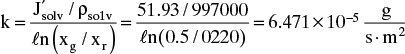
Now solve Eq. (18-42) with xin = 0.20 and xout = 1.5xin = 0.30.
Final result is ![]()
E. Check. Qualitatively we expect a lower flux since there are more latex particles carried toward the wall per liter of fluid, which permeates through the membrane. Other than checking the equations and calculations, a check is difficult.
F. Generalize.
1. We have assumed k is not concentration dependent. This is reasonable for particles.
2. If a correlation for k was available, we could use Eq. (18-42) and J′solv to estimate xg.
3. The general procedure was to:
a. Use a rearranged design equation to find a design parameter (k) using experimental conditions.
b. Use a design equation to predict flux under the design conditions.
This general procedure is very common in all types of separation problems.
4. It is critically important to determine whether a gel layer forms.
Warning! Experimental results and equations for both UF and RO are reported in many different units. It is easy to make a unit mistake if you do not carefully carry units in the equations. It is especially easy to make a subtle mistake in the appropriate solution density to use when converting from concentration c in g/L or mole/L to weight fraction x. The correct conversion from g/L to weight fraction is

Unfortunately, the solution density ρsolution is a function of concentration. For a relatively pure permeate (R close to 1.0) the permeate solution density is approximately the solvent density. For more concentrated streams, such as the feed or the retentate, the density needs to be known or estimated as a function of concentration.
When concentrations are given in units of g/L, approximations are often made to calculate fluxes. For example, the correct equation for the solute mass flux is

This is often approximated as

For relatively high rejection coefficients permeate is quite pure, Jsolv >> JA, and the approximation is quite good. In other cases the approximation may not be as accurate.
The inherent rejection and concentration polarization modulus are often defined in concentration units:
With these definitions the solute mass flux is
Equations (18-46) and (18-47) are valid ways to formulate the problem. Unfortunately, it may be assumed that ![]() and M = Mc when the exact equations are
and M = Mc when the exact equations are


If ρsolution,out and ρsolution,p are very different, confusing R with Rc and M with Mc can result in significant error. To be exact, check how all terms are defined, use the appropriate solution densities of permeate and retentate to convert to weight fraction units, and then solve in weight fraction units.
18.6 Pervaporation (Pervap)
Pervaporation can be traced back to Graham’s work in the 1860s, but definitive work was done by Binning in the 1950s and 1960s, with first commercialization for ethanol purification in the 1980s (Baker et al., 1990). The very long time to commercialization occurred because membranes did not have a combination of high flux, high selectivity, and long life that would make them economically viable. With current membranes pervap is of interest because very high selectivities with reasonable fluxes are often obtained. In pervap a high-pressure liquid is fed to one side of the membrane, and one component preferentially permeates across the membrane and evaporates on the downstream side, and vapor permeate is withdrawn (Figure 18-13). The word pervaporation is a contraction of permeation and evaporation. Retentate, which does not permeate through the membrane, is a high-pressure liquid product. Either permeate or retentate may be valuable product.
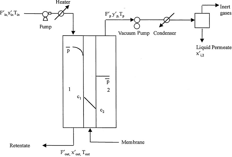
18.6.1 Pervap Basics
Since both selective membrane permeation and evaporation occur, pervap both separates and concentrates. The driving force is adequately represented by the partial pressure difference across the membrane. Local partial pressure on the upstream side, labeled 1 in Figure 18-13, is
while local partial pressure on the downstream side, labeled 2, is
and local driving force is
Because xi,1, yi,2, and ptot,2 vary, local values of partial pressures and driving force depend on flow patterns and pressure drop in the membrane module.
Driving force can be increased by lowering ptot,2 either by drawing a vacuum as shown in Figure 18-13 or, less frequently, by reducing yi,2 using a sweep gas on the permeate side. Driving force will also be increased if upstream partial pressure of component i is increased. This occurs for more concentrated feeds (higher xi,1) and at higher upstream temperatures (larger VPi,1). Use of higher upstream temperatures may require a higher upstream pressure to prevent vaporization of liquid on the upstream side. Higher upstream pressure does not increase the permeation rate significantly (Neel, 1991). Although feed concentration is not usually a variable the designer can control in a stand-alone, single-pass system (Figure 18-13), it is a design variable in hybrid systems (Figure 18-14).
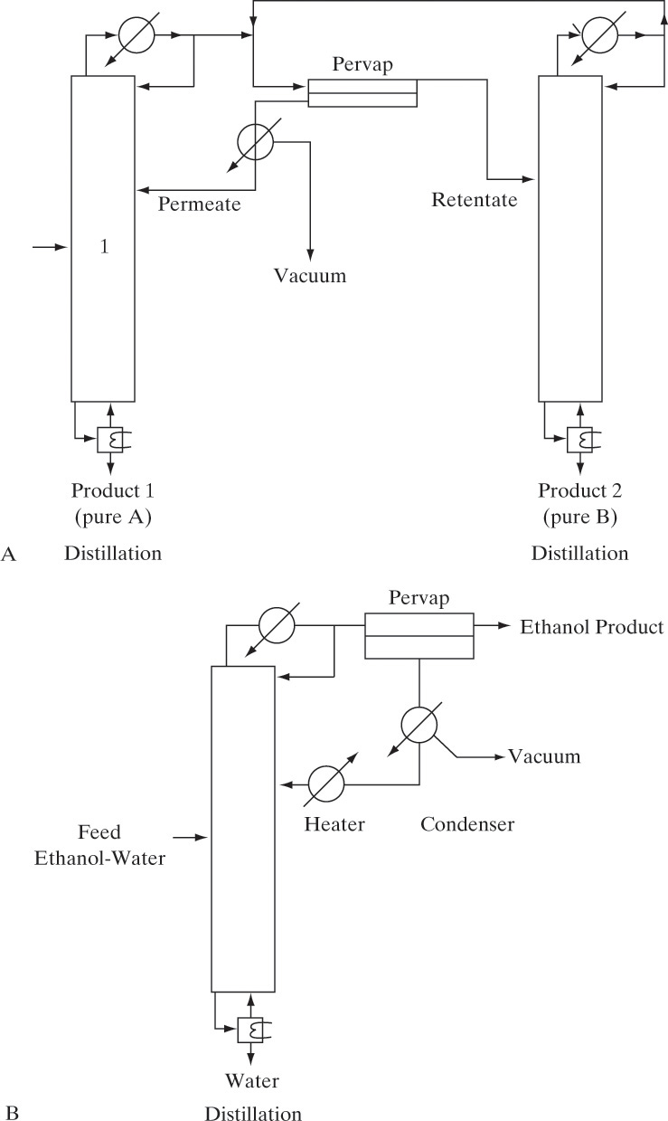
FIGURE 18-14. Hybrid pervap system coupled with distillation; (A) general two-column system, (B) simplified one-column system shown for dehydration of ethanol
As usual with membrane separations, the membrane is critical for success. Currently, two different classes of membranes are used commercially for pervap. To remove traces of organics from water a hydrophobic membrane, most commonly silicone rubber coated on a microporous support, is used. To remove traces of water from organic solvents a hydrophilic membrane such as cellulose acetate, ion exchange membranes, polyacrylic acid, chitosan or Nafion® is used. Both types of membranes are nonporous and operate by a solution-diffusion mechanism. Selecting a membrane that will preferentially permeate the more dilute component will usually reduce the membrane area required. Membrane life is typically about four years (Baker, 2004).
Because evaporation increases the driving force, pervap can use a highly selective membrane and retain a reasonable flux if the more permeable component is also more volatile. However, evaporation complicates both equipment and analysis. Typical permeate pressures are quite low (0.1–100 Pa) (Leeper, 1992). Because of this low pressure, the permeate needs a large cross-sectional area for flow or the pressure drop caused by flow of permeate vapor will be large. Thus, plate and frame, spiral wound, and hollow fibers with feed inside the fibers are used commercially. Figure 18-13 shows that a vacuum pump and a condenser may both be required to recover dilute low-pressure vapor. Unless the cut is small, an additional energy source is required to supply heat of evaporation. If the cut is small, energy in the hot liquid can supply this energy. For larger cuts a portion of retentate can be heated and then recycled. Huang (1991) discusses equipment and equipment design, and Baker (2012) outlines several pervap processes.
Although selectivity in pervap units can be quite high (e.g., Leeper [1992] reports values from 1.0–28,000), the values are not infinite. There will always be some less permeable species in the permeate and some more permeable species in the retentate. If feed concentration and selectivity are high enough, a single-pass system (Figure 18-13) can produce high-purity permeate or high-purity retentate. However, the other stream will contain a significant amount of valuable product. Single-pass systems can produce high purity or high recovery but not both simultaneously.
If both high purity and high recovery are desirable or a single-pass system cannot meet product specifications, a hybrid system with recycle is often used (Huang, 1991; Suk and Matsura, 2006; Wankat, 1990). Hybrid systems use two different types of separation. The most common pervap hybrid is to combine it with distillation with either two columns (Figure 18-14A) or a single column (Figure 18-14B). In Figure 18-14A feed to distillation column 1 forms a minimum-boiling azeotrope. Bottoms product is essentially pure component A. Distillate product from column 1, which approaches the azeotrope concentration, is fed to the pervap unit. If component A preferentially permeates the membrane, the permeate will be more concentrated in A than the distillate. The permeate is then recycled to column 1 to recover the A product. Component B is concentrated in the retentate, which is fed to distillation column 2. Distillate from column 2 also approaches the azeotrope concentration and is part of the feed to the pervap unit. Bottoms product from column 2 is essentially pure B. The two distillation columns in Figure 18-14A are similar to the columns in Figure 8-4A. Since the pervap unit replaces the liquid-liquid separator in Figure 8-4A, the hybrid system does not require a heterogeneous azeotrope; thus, Figure 18-14A is more generally applicable.
If the selectivity is high enough, the retentate may meet purity specifications. Then distillation column 2 is not needed, which results in obvious savings in capital and operating costs. This is illustrated with a simplified one-column flowchart used for breaking the ethanol-water azeotrope (Figure 18-14B). Open steam heating may be used instead of a reboiler (Leeper, 1992). A hydrophilic membrane that selectively permeates water is used. This figure is similar to Figure 8-3A with the pervap system replacing the liquid-liquid separator.
Hybrid system pervap units are usually designed with a low cut per pass to prevent a large temperature drop. Total cut for the entire unit can be any desired value. Typically, if required, a vacuum pump is the highest operating expense. Vacuum pump load can be decreased by refrigerating the permeate condenser’s final stage. Appropriate design of heat exchangers and thermally integrating pervap and distillation systems can significantly reduce energy costs.
18.6.2 Pervap Design Using Experimental Data
Pervap units are often designed from experimental selectivity and flux data. For a binary system separation factor βA,B is defined as

Because separation factor data are often reported in weight units, in this section we define x and y as weight fractions in liquid and vapor, respectively. Molar units can also be used and are preferred for theoretical analysis (Baker et al., 2010). Equation (18-50) is superficially similar to the definition of relative volatility in distillation. Of course, here the separation factor is for a rate process and represents the RT curve, not equilibrium. Separation factor data are usually obtained under conditions where concentration polarization is negligible. Experimentally determined separation factors are functions of temperature and liquid mole fraction (e.g., see Figure 18-15).
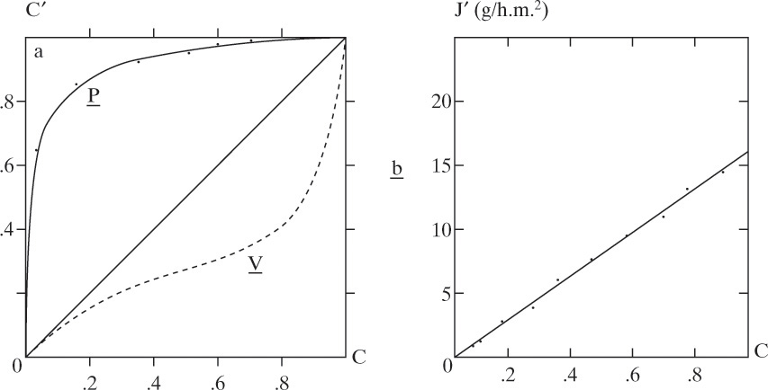
FIGURE 18-15. Vacuum-pervaporation of water-ethanol mixtures through homogeneous films made from hydrophilic polymer; a. Water weight fraction in liquid [c] and in permeate [c′]; b. (J′) Permeation flux, polyacrylonitrile film (20.0 µm thick), T = 25.0°C; (Neel, 1991), copyright 1991. Reprinted with permission from Elsevier.
Separation factor data can be converted to y versus x format by solving for yA in Eq. (18-50b):

Since separation factor usually depends on liquid concentration, Eqs. (18-50a) to (18-50c) are valid locally.
We again use membrane modules that are well mixed on both the retentate and permeate sides. In this situation Eq. (18-50c), with y replaced by yp and x replaced by xout, becomes the RT equation
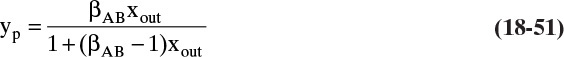
where yp and xout refer to weight fractions of the more permeable component in the permeate and the retentate, respectively. Selectivity β in Eq. (18-51) must be determined at operating temperature T and liquid weight fraction xout. If data are available in the form of Figure 18-15, it must be at operating temperature, T, of the pervap system.
The overall mass balance for a single-pass system (Figure 18-13) is
and the mass balance for the more permeable species is
These equations are identical to the balances for gas permeation, Eqs. (18-7a) and (18-7b), except that x has replaced y for feed and retentate. Solving Eqs. (18-52a) and (18-52b) simultaneously for yp

where cut θ′ = F′p/F′in. This result is essentially the same as Eq. (18-8). If we want to use a graphical procedure, the operating equation will plot as a straight line on a graph of yp vs. xout.
If xout and T are specified (which means βAB is known), Eqs. (18-51) and (18-53) can be solved simultaneously. The resulting equation is quadratic in yp and linear in θ′ (Wankat, 1990, pp. 707–709). Unfortunately, this procedure is more complicated and less useful in real situations than it appears at first glance. Since neither xout nor T is usually known, selectivity is not known, and the calculation becomes complicated. We will use a simultaneous graphical solution to develop a somewhat simpler procedure that is illustrated in Example 18-10.
An energy balance is needed to estimate pervap system temperature. We assume that the pervap system is adiabatic and is operating at steady state. Then the energy balance for the system shown in Figure 18-13 is
We choose pure liquid component A at temperature Tref as the reference. Assuming heat of mixing is negligible, enthalpies of liquid streams are
and vapor enthalpy is
where λp is mass latent heat of vaporization of the permeate determined at Tref, and heat capacities are also in mass units. Combining Eqs. (18-54a) to (18-54c), we obtain
Since the membrane module is well mixed, it is reasonable to assume the system is in thermal equilibrium, Tout = Tp. If we arbitrarily set reference temperature equal to outlet temperatures, Tref = Tout = Tp, we obtain simplified forms of the energy balance.
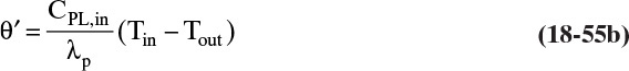
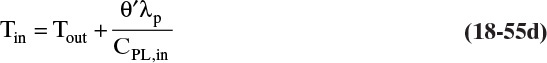
From Eq. (18-55b) we can determine the cut necessary to obtain a specified outlet temperature, and Eq. (18-55c) allows us to determine outlet temperature for any specified cut. The relationship between cut and temperature drop of the liquid stream is linear. Examining Eq. (18-55c) is instructive. Since latent heat is significantly greater than heat capacity, outlet temperature drops rapidly as cut is increased. To prevent this drop in temperature a recycle system with a low cut per pass is often used.
We are now ready to develop the solution procedure for completely mixed pervap systems. This procedure is straightforward if selectivity data are available and either outlet temperature or cut are specified. If cut is specified, calculate Tout from Eq. (18-55c). To plot the RT curve, pick arbitrary values for xout, calculate βAB from appropriate data such as Figure 18-15 or 18-16, calculate yp from RT Eq. (18-51), and plot the point on the curve. If experimental y vs. x data at operating temperature T are available, plot it directly as yp vs. xout. The simultaneous solution to the selectivity equation and mass balances is at the point of intersection of the RT curve and the straight operating line, Eq. (18-53) (see Figure 18-16 in Example 18-10).
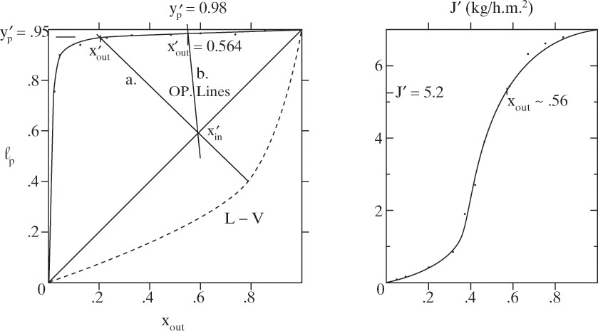
FIGURE 18-16. Solution for Example 18-10; RT curve for water-ethanol through 20.0 µm polyvinyl alcohol at 60.0°C. (Neel, 1991). Flux curve from Neel (1991), copyright 1991. Reprinted with permission from Elsevier.
EXAMPLE 18-10. Part I. Pervaporation—feasibility calculation
You are asked by a client to develop a single-pass pervaporation system to separate water from ethanol using a 20.0 micron–thick polyvinyl alcohol film. The perfectly mixed pervaporation system will operate at 60.0°C with 1000.0 kg/h of hot feed. The feed is 60.0 wt% water. The client wants a retentate product that is 20.0 wt% water. Is this process feasible?
A. Define. In this case, feasibility means: can the process be conducted with the feed at a reasonable temperature? Thus, to determine feasibility we need to determine the required inlet temperature.
B, C. Explore and Plan. Rate transfer information and flux data for this membrane are given by Neel (1991) and are shown in Figure 18-16. Data required for energy balances are available in Perry and Green (1997) on pages 2-235 and 2-306:
Ethanol: CP,L,E = 2.78 kJ/(kg K) and λE = 985 kJ/kg. Estimated at 60.0°C.
Water: CP,L,W = 4.185 kJ/(kg K) and λW = 2359 kJ/kg. Estimated at 60.0°C.
After solving for cut and feed temperature, we discuss feasibility.
D. Do it. Data from Neel (1991) are plotted in Figure 18-16. The operating line (not shown by Neel), Eq. (18-56), goes through point yp = xout = xin, which is on y = x line. To meet the required retentate concentration, operating line must intersect the RT curve at xout = 0.20. Permeate weight fraction can be read at this point as yp = 0.95 weight fraction water. Since all weight fractions are known, it is easiest to simultaneously solve Eqs. (18-52a) and (18-52b) for cut, θ′.
Result is θ′ = (0.6 – 0.2)/(0.95 – 0.2) = 0.533. Since typical values for cut are approximately 0.1 or less, it is highly likely that this design is not feasible; however, we need to solve for feed temperature to prove the design is not feasible. To check for feasibility, we can use energy balance Eq. (18-55d) to estimate the required inlet temperature. Latent heat of the permeate can be estimated as
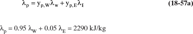
Heat capacity of feed at 60.0°C can be estimated as
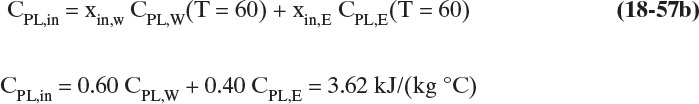
Then from Eq. (18-55d), Tin = 60 + (0.533)(2290)/(3.62) = 396.9°C.
This is obviously too hot. The process is not feasible because the membrane will be thermally destroyed, and the feed will not be a liquid. Too large a cut is used.
E. Check. Since typical values for cut are approximately 0.1 or less, our conclusion that the process is not feasible is reasonable.
F. Generalization. Example 18-10 illustrates that operation of single-pass pervaporation units is controlled by the simplified energy balance, Eq. (18-59c). Essentially, there must be sufficient energy in the feed liquid to vaporize the desired fraction of the feed. High cuts require very hot feeds to supply the energy needed for vaporization.
Part B: Development of a feasible design
Since the operation in Part A was not feasible, choose an appropriate feed temperature, and develop a feasible pervaporation process for feed in Part A. A permeate that is greater than 95.0 wt% water is desired. Retentate concentration is not specified. Determine cut, permeate and retentate weight fractions, and membrane area.
Solution
A. Define. An appropriate feed temperature is within the temperature limits of the membrane, and feed must be liquid at a reasonable pressure. There is no single correct answer.
B, C. Explore and plan. A pressurized feed will still be liquid at 120.0°C. With a smaller cut, permeate will be greater than 95.0% water. If cut were zero, the operating line would be vertical. From Figure 18-16, yp = 0.98. We can use yp = 0.98 to estimate λp, which is needed to calculate cut. The accuracy of this estimate can be checked when we are finished.
D. Do it. Estimate the latent heat of vaporization of the permeate product (yp = 0.98) as λp = 0.98 λW + 0.02 λE = 2331 kJ/kg. Value of CPL,in = 3.62 kJ/(kg °C) was determined in Part A. Then from Eq. (18-55b)
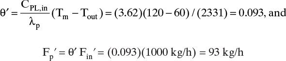
From Eq. (18-53) operating line has a slope = –(1.0 – 0.093)/0.093 = –9.75. The operating line is drawn in Figure 18-16. The permeate weight fraction is about 0.98 (thus, our approximation was accurate), and the retentate weight fraction is slightly above 0.56.
Membrane flux can be determined from the flux part of Figure 18-16. J′ is about 5.2 kg/(h m2). Then membrane area = F′p/J′ = 93/5.2 = 16.9 m2.
F. Generalization. At this retentate liquid concentration the membrane has a high flux. At the original retentate value, xout = 0.2 used in Part A, the flux is much lower, and significantly more membrane area is required.
Of course, there are many different feasible designs. If a higher permeate concentration is desired, the ethanol-water feed mixture in Example 18-10 would probably be concentrated in an ordinary distillation column to a concentration much closer to the azeotrope concentration (see Figure 18-14B). Retentate is typically recycled to the distillation column. Pervaporation, azeotropic distillation (Chapter 8), and adsorption (Chapter 19) are all used commercially to break the ethanol-water azeotrope.
18.6.3 Theoretical Design of Pervap Systems
Baker et al. (2010) argue vigorously that the traditional approach of presenting pervap data as flux and separation factor (e.g., Figure 18-17) obscures the fundamentals behind separation and makes comparison of data from different sources very difficult. Because liquid is in equilibrium with vapor that has evaporated, pervaporation and vapor permeation processes are very similar; thus, Eqs. (18-2b) and (18-2c), written in terms of partial pressures, can be employed (Baker, 2012). Volumetric flux equations for JA and JB are

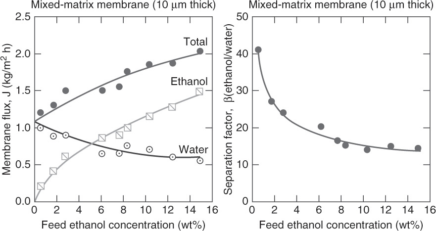
FIGURE 18-17. Flux and ethanol/water separation factor data obtained with 10.0 µm zeolite (60.0 wt%)—silicone rubber mixed-matrix membrane with flow through test cells, 75.0°C, permeate pressure < 5.0 Torr, stage-cut per cell of less than 0.2%. Reprinted with permission from Baker et al., “Permeability, Permeance and Selectivity: A Preferred Way of Reporting Pervaporation Performance Data,” J. Membrane Sci., 348 (1–2), 346–352 (2010). Copyright 2010, Elsevier.
The corresponding molar flux equations are

There are two important differences between Eq. (18-58a) and Eq. (18-2c). First, pA,1 is calculated from Eq. (18-49a), pA,1 = xA,1(VP)A,1, in pervap, while retentate partial pressure in vapor permeation is calculated from pA,r = yA,r ptotal,r. Vapor pressure of A in a binary mixture can be calculated from
Equation (18-59) requires vapor pressure of pure component and activity coefficient γA, which depends on the binary mixture, mole fraction xA, and temperature, T. Pure component vapor pressures and correlations of these vapor pressures in terms of Antoine equation constants are readily available in handbooks. If component A is water, steam tables provide very detailed tables of saturation pressure (called vapor pressure). Activity coefficient γA (xA, T) can be determined with an appropriate equation of state. Since process simulators calculate activity coefficients while calculating VLE, activity coefficients can be conveniently determined with a process simulator (see Example 18-11).
Based on Equations (18-58) pervaporation flux data should be reported as permeabilities, or if membrane thickness is not known, as permeances, P/tms (Baker et al., 2010). Ability of the system to separate the two components should be reported as selectivity, αAB, defined for gas permeation in Eq. (18-4b).
The second major difference between the pervap and vapor permeation equations is permeability in pervap depends on both evaporation (vapor-liquid equilibrium) and permeation through the membrane, whereas in vapor permeation, permeation occurs only through the membrane. The separation factor for pervap can be calculated as the product of separation factors for evaporation and for membrane permeation (Baker, 2012).
EXAMPLE 18-11. Analysis of pervap data
The pervap data in Figure 18-17 is presented in terms of ethanol and water fluxes and separation factor.
A. Convert flux data for 12.0 wt% ethanol feed to ethanol and water permeabilities and selectivity αE–W.
B. Determine separation factors β for 12.0 wt% ethanol feed due to evaporation and vapor permeation.
Solution
Part A. First, convert weight fractions of feed to mole fractions. Ethanol is 5.07 mol% (MW = 46), and water is 94.93 mol%.
Second, read fluxes as accurately as possible: Water flux = 0.625 and ethanol = 1.3125 kg/(m2 h). Then convert to molar fluxes: JM,E = 0.02853 and JM,W = 0.03461 kmol/(m2 h).
Third, read selectivity as carefully as possible: βE,W = 14.375. Then from Eq. (18-50c)
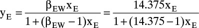
Since cut in Figure 18-17 is very low, feed concentration is essentially identical to retentate concentration. Calculating yE for xE = 0.0507, yE,pervap = 0.4343.
Fourth, solve Eqs. (18-58a) and (18-58b) for permeabilities PA and PB:

Fluxes were calculated in step 2, tms = 10.0 µm = 10.0 × 10⁻⁶ m. The pressure was 5.0 torr:
P2,total = (5.0 torr)[(1.0 atm)/(760.0 torr)][(101.3 kPa)/(1.0 atm)] = 0.6664 kPa
At this low pressure gases are ideal, and molar densities are
ρM,E = ρM,W = ρM = 1.0 mol/22.4 L (STP) = 1.0 kmol/22.4 m3 (STP).
The downstream partial pressures, pi,2 = yi P2,total are
pE,2 = yE P2,total = (0.4343)(0.6664 kPa) = 0.2894 kPa, and pW,2 = 0.3770 kPa.
From Eqs. (18-49a) and (18-59) pE,1 = xE,1 γE VPpure E and pW,1 = xW,1 γW VPpure W. From the steam tables, the vapor pressure of pure water at 75.0°C = 38.60 kPa. The NIST WebBook (webbook.nist.gov) gives the Antoine coefficients for ethanol: A = 5.24677, B = 1598.673, and C = –46.424 for Antoine equation form log10(VP) = A – (B/[T + C]) with VP in bar and T in K. Calculated vapor pressure of pure ethanol at 75.0°C is 88.822 kPa.
Activity coefficients γE and γW are calculated by process simulators. In Aspen Plus activity coefficients can be determined as follows: Open Aspen Plus, and input ethanol and water as the components. Choose a suitable VLE correlation such as NRTL. Run properties/analysis set-up. Go to Binary Analysis on the toolbar. Select p-xy analysis. Set temperature to 75.0°C, and request 100 points. Run the analysis. A p-xy diagram will appear. In the left-hand menu, click Results under Analysis BINRY-1. A table will appear that gives values of activity coefficients (labeled LIQUID GAMMA ETHANOL and LIQUID GAMMA WATER [assuming ETHANOL and WATER are the component names you selected]). We want γE at ethanol mole fraction in feed, xE = 0.0507. From the table generated by Aspen Plus, at 0.05 mole fraction γE = 4.08646 and at 0.06 mole fraction γE = 3.89066. By linear interpolation at xE = 0.0507, γE = 4.0728. A similar calculation is done for water: at xW = 0.9493, γW = 1.0070. Then
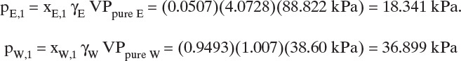
From these values we can calculate permeabilities:
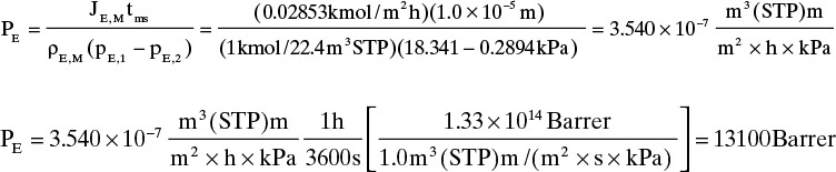
The corresponding calculation for water gives PW = 7840.0 Barrer.
Part B. The separation factor for evaporation is
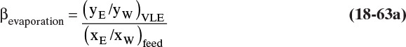
The equilibrium values for yE and yW can be obtained from the same Aspen Plus table used to find the gamma values at 75.0°C. Then
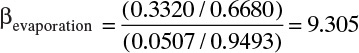
The separation factor for permeation is
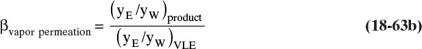
The product values for yE and yW were calculated in part a, and the VLE values were determined from the Aspen Plus table.
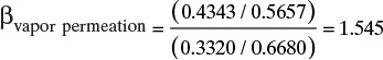
βpervap = βevaporation βpermeation = (9.305)(1.545) = 14.375, which is the value read from Figure 18-17.
Check: Permeability values reported by Baker et al. (2010) are ∼11,100 Barrer for ethanol and ∼7000.0 Barrer for water. Values calculated in this example are within 18.0% for ethanol and 12.0% for water. A significant amount of this error is probably from reading the figures to obtain values for fluxes, β, and permeabilities calculated by Baker et al. (2010).
18.7 Bulk Flow Pattern Effects
Completely mixed membrane systems are relatively common in laboratory units since effects of concentration polarization and gel formation can be minimized or eliminated. Commercial units usually use one of the modules shown in Figure 18-1 since a large membrane area can be packaged in a small volume. Flow patterns of bulk fluid in these modules are unlikely to be perfectly mixed and are more likely to approximate crossflow (Figure 18-18A), cocurrent (Figure 18-18B), or countercurrent (Figure 18-18C) flow. Since these bulk flow patterns all result in better separation than a perfectly mixed module, our previous results are conservative estimates. In this section we analyze an ideal example (that is with no axial mixing and no concentration polarization) for gas permeation for crossflow to determine the improvement in separation. Results for cocurrent and countercurrent flow are discussed, but detailed analyses are not presented. Because real systems usually have some axial mixing, separation is often between that predicted for the ideal flow pattern and the perfectly mixed case.
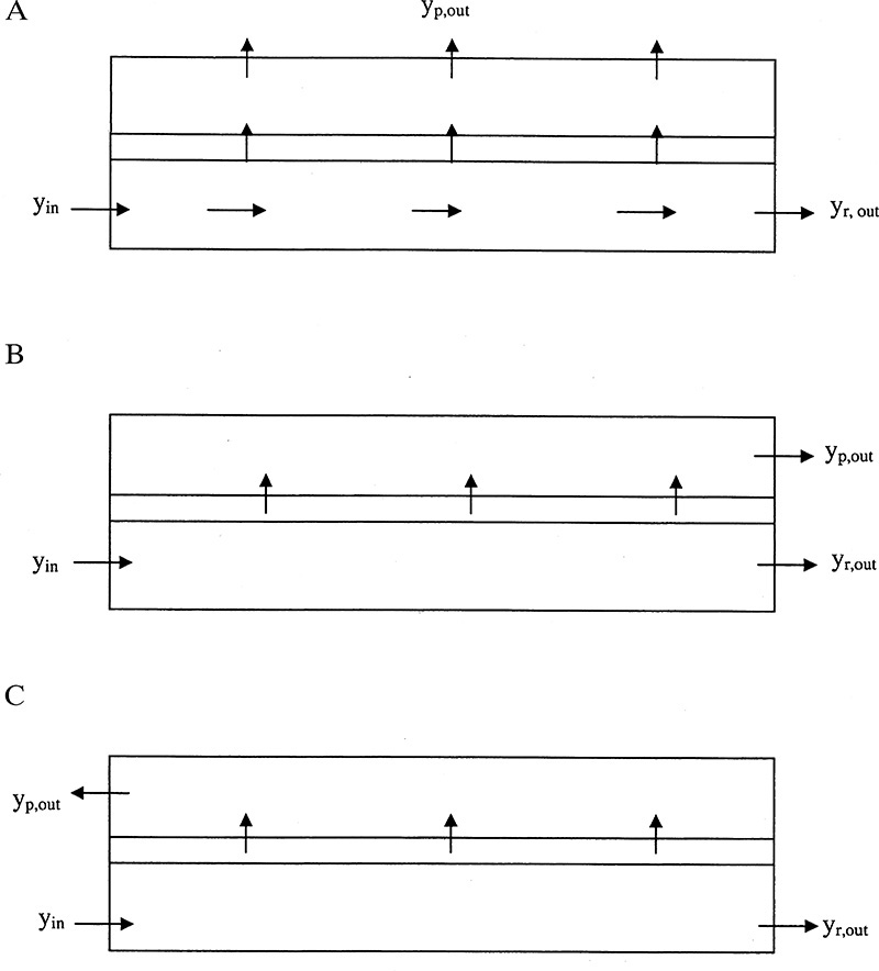
FIGURE 18-18. Flow patterns in gas permeation systems; (A) crossflow with unmixed permeate, (B) cocurrent flow, (C) countercurrent flow
EXAMPLE 18-12. Flow pattern effects in gas permeation
The increase in separation for different flow patterns can be compared for separation of oxygen and nitrogen. Geankoplis (2003) presents a problem with a feed that is 20.9% oxygen, pr = 2.5 and pp = 0.25 atm, PO2/tms = 1.9685 × 10⁻⁵ cm3(STP)/[cm2.s.cm Hg], αO2-N2 = 10.0, Fin = 1,000,000 cm3 (STP)/s, and cut = 0.20. Results shown in Table 18-3 were obtained with spreadsheets, Mathematica (Binous, 2006), and detailed analytical solutions (Geankoplis, 2003). They illustrate that a countercurrent flow pattern provides better separation with less membrane area than the alternatives.
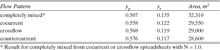
TABLE 18-3. Results for oxygen mole fractions for different flow patterns in gas permeation systems.
It is convenient to use staged models (Figure 18-19) to analyze these flow patterns. Essentially, use of staged models is a numerical integration of the differential equations. Coker et al. (1998) developed programs to solve the simulation problem (area is known) to find cut, outlet flow rates, and mole fractions.
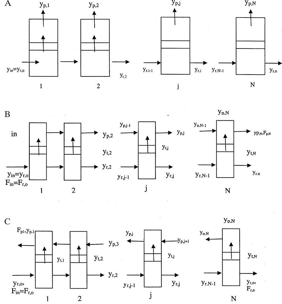
FIGURE 18-19. Staged models for different flow patterns in gas permeation; (A) crossflow system, (B) cocurrent system, (C) countercurrent system
18.7.1 Binary Crossflow Permeation
Spiral-wound membrane units are very close to crossflow operation with an unmixed permeate (Figure 18-18A). We can approximate this crossflow system as a series of N well-mixed stages as shown in Figure 18-19A. Since we know how to solve each well-mixed stage in Figure 18-19A, we can add results to find the behavior of the crossflow system. A complicated analytical solution exists for binary crossflow gas permeation (Geankoplis, 2003), allowing us to check the accuracy of our numerical solution.
For a design problem (cut is specified and membrane area is unknown) solution is easiest if we make permeate flow rate, Fp,j, for each small, well-mixed stage the same Fp,j = Fp; thus, each stage has different areas. Then flow rates from the crossflow system are
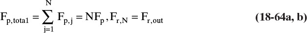
Since stages are well-mixed and rapid mass transfer is assumed, yr = yr,w. We can write Eqs. (18-6a) and (18-8a) for each small, well-mixed stage j using variables yp,j, yr,j (both for more permeable component), Fm,p, and Fm,r,j. For constant selectivity these equations can be solved simultaneously by substituting Eq. (18-8a) in (18-6a), rearranging, and solving with the quadratic equation. The resulting solutions for each stage are identical to Eqs. (18-10) (in Example 18-2), except yin is replaced with yr,j–1, and θ is replaced by
We can substitute volumetric rate, Fp, for molar rate, Fm,p, because volumetric flow rates in cm3(STP)/s are equivalent to molar flow rates. Retentate flow rates and retentate mole fractions for each stage can be found from external mass balances, Eq. (18-7), which can also be written in terms of volumetric flow rates in cm3(STP)/s. (Remember: For ideal gases, mole fraction = volume fraction.) Then outlet retentate volumetric flow rate and mole fraction are
Starting with stage j = 1, the solution procedure is as follows: Quadratic Eq. (18-10), which results from simultaneous solution of RT and operating equations, is solved on stage j for yp,j. Since Fp and Fr,j–1, feed flow rate to stage j, are known, and yp,j was just calculated, Eqs. (18-65a) and (18-65b) can be solved to determine Fr,j and yr,j. The area Aj for each stage can be determined by rearranging Eq. (18-5a) and substituting Fp = Fm,p/ρm,p:
The counter j is increased by 1, which makes the previously calculated values the values for j – 1, and the process is repeated.
Once every stage has been calculated, the mole fractions for the crossflow system are
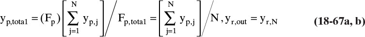
and the total area is
This set of equations is easy to program within a mathematical package. If N is large enough (N = 1000 is more than sufficient and requires little time) very good agreement will be obtained with the analytical solution, with less effort and less time. Numerical solution methods can easily include a variable selectivity. A spreadsheet program and example are in this chapter’s appendix.
Crossflow systems with unmixed permeate have more separation than completely mixed systems. Crossflow works better than well mixed because average driving force, [∑(pryr,j – ppyp,j)]/N, is considerably larger in crossflow than the single driving force, (pryr,out – ppyp), in well-mixed systems. A real system probably has some but not complete mixing on both the permeate and retentate sides; thus, the permeate mole fraction is probably between the values calculated for completely mixed and crossflow.
The analysis for crossflow can be extended to multicomponent systems. Now each stage is a perfectly mixed multicomponent system with a feed from the previous stage. The results for each stage can be calculated using the procedure in Section 18.3.3. Thus, a trial-and-error procedure is needed on each stage, but the entire cascade is calculated only once. Coker et al. (1998) illustrate a different procedure for multicomponent crossflow.
18.7.2 Binary Cocurrent and Countercurrent Permeation
Tubular and hollow-fiber membrane systems can be operated in cocurrent flow (Figure 18-18B) or in countercurrent flow (Figure 18-18C). Both flow patterns can be analyzed with a staged model similar to that used for crossflow. The cocurrent model is shown in Figure 18-19B. Note that permeate streams from all stages left of stage j are mixed together, and the resulting mixture is permeate for stage j. This flow pattern is used to calculate new permeate mole fraction yp,j. Permeate mole fraction transferring through the membrane is determined from solution of Eq. (18-10). This model again represents a numerical integration of differential equations. Coker et al. (1998) present a solution method for multicomponent permeation when the membrane area is known but cut is unknown.
Tubular and hollow-fiber modules can be arranged to have approximately countercurrent flow patterns (Figure 18-18C). Since countercurrent flow is an advantage in equilibrium-staged systems, we would expect that it might be advantageous in membrane separations also. Example 18-12 shows that this is true. A staged model for countercurrent flow is shown in Figure 18-19C. Note that permeate streams from all stages right of stage j are mixed together, and the resulting mixture is permeate for stage j. This flow pattern is used to relate permeate mole fraction yp,j to the permeate mole fraction transferring through the membrane plus permeate from later stages, yp,j+1. Since later stages have not been calculated yet, the analysis requires trial and error. Coker et al. (1998) present a solution method for a staged model for countercurrent, multicomponent permeation when the membrane area is known but cut is unknown.
Students interested in computer programs to solve cocurrent and/or countercurrent gas permeation are referred to Coker et al. (1998) or the third edition of Separation Process Engineering (Wankat, 2012).
Baker, R. W., “Membrane Technology,” in A. Seidel (Ed.), Kirk-Othmer Encyclopedia of Chemical Technology, 5th ed., Vol. 15, Wiley-Interscience, New York, 2004, pp. 796–852.
Baker, R. W., and I. Blume, “Permselective Membranes Separate Gases,” Chem. Tech., 16, 232 (1986).
Baker, R. W., E. L. Cussler, W. Eykamp, W. J. Koros, R. L. Riley, and H. Strathmann, Membrane Separation Systems, U.S. Department of Energy, DOE/ER30133-H1, April 1990, Reprinted by Noyes Data Corp., Park Ridge, NJ, 1991.
Baker, R. W., J. G. Wijmans, and Y. Huang, “Permeability, Permeance and Selectivity: A Preferred Way of Reporting Pervaporation Performance Data,” J. Membrane Sci., 348 (1–2), 346 (2010).
Binous, H., “Gas Permeation Computations with Mathematica,” Chem. Eng. Educ., 140 (Spring 2006).
Bird, R. B., W. E. Stewart, and E. N. Lightfoot, Transport Phenomena, Revised 2nd ed., Wiley, New York, 2006.
Blatt, W. F., A. Dravid, A. S. Michaels, and L. Nelson, “Solute Polarization and Cake Formation in Membrane Ultrafiltration: Causes, Consequences and Control Techniques,” in J. E. Flinn (Ed.), Membrane Science and Technology, Plenum Press, New York, 1970, pp. 47–97.
Cath, T. Y., A. E. Childress, and M. Elimelech, “Forward Osmosis: Principles, Applications, and Recent Developments,” J. Membrane Sci., 281, 70–87 (2006).
Chern, R. T., W. J. Koros, H. B. Hopfenberg, and V. T. Stannett, “Material Selection for Membrane-Based Gas Separations,” in D. R. Lloyd (Ed.), Materials Science of Synthetic Membranes, Am. Chem. Soc., Washington, D. C., Chapter 2, 1985.
Chung, T.-S., S. Zhang, K. Y. Wang, J. Su, M. M. Ling, “Forward Osmosis Processes: Yesterday, Today and Tomorrow,” Desalination, 287, 78–81 (2012).
Coker, D. T., B. D. Freeman, and G. K. Fleming, “Modeling Multicomponent Gas Separation Using Hollow-Fiber Membrane Contactors,” AChE Journal, 44, 1289 (1998).
Conlee, T. D., H. C. Hollein, C. H. Gooding, and C. S. Slater, “Ultrafiltration of Dairy Products in a ChE Laboratory Experiment,” Chem. Eng. Educ., 32 (4), 318 (Fall 1998).
Drioli, E., and M. Romano, “Progress and New Perspectives on Integrated Membrane Operations for Sustainable Industrial Growth,” Ind. Engr. Chem. Research, 40, 1277 (2001).
Eykamp, W., “Membrane Separation Processes,” R. H. Perry and D. H. Green (Eds.), Perry’s Chemical Engineers’ Handbook, 7th ed., McGraw-Hill, New York, pp. 22-37 to 22-69, 1997.
Foley, G., “The Lambert W Function in Ultrafiltration and Diafiltration,” Chem. Engr. Educ., 50 (2), 107 (2016).
Geankoplis, C. J., Transport Processes and Separation Process Principles (Includes Unit Operations), 4th ed., Prentice Hall, Upper Saddle River, NJ, 2003, Chapter 13.
Geraldes, V., N. E. Pereira, and M. Norberta de Pinho, “Simulation and Optimization of Medium-Sized Seawater Reverse Osmosis Processes with Spiral-Wound Modules,” Ind. Engr. Chem. Research, 44, 1897 (2005).
Green, D. W., and R. H. Perry (Eds.), Perry’s Chemical Engineers’ Handbook, 8th ed., McGraw-Hill, New York, 2008.
Henis, J. M. S., and M. K. Tripodi, “The Developing Technology of Gas Separating Membranes,” Science, 220 (4592), 11 (April 1, 1983).
Ho, W. S. W., and K. K. Sirkar (Eds.), Membrane Handbook, Van Nostrand Reinhold, New York, 1992.
Hoffman, E. J., Membrane Separations Technology: Single-Stage, Multistage, and Differential Permeation, Gulf Professional Publishing (Elsevier Science), Amsterdam, 2003.
Huang, R. Y. M. (Ed.), Pervaporation Membrane Separation Processes, Elsevier, Amsterdam, 1991.
Kesting, R. E., and A. K. Fritzsche, Polymeric Gas Separation Membranes, Wiley, New York, 1993.
Kucera, J., Reverse Osmosis: Industrial Applications and Processes, Scrivener Publishing, Salem, MA, 2010.
Leeper, S. A., “Membrane Separations in the Recovery of Biofuels and Biochemicals: An Update Review,” in N. N. Li and J. M. Calo (Eds.), Separation and Purification Technology, Marcel Dekker, New York, 1992, pp. 99–194.
Leeper, S. A., D. H. Stevenson, P. Y.-C. Chiu, S. J. Priebe, H. F. Sanchez, and P. M. Wikoff, Membrane Technology and Applications: An Assessment, U.S. Department of Energy, February 1984.
Li, N. N., and S. S. Kulkarni, “Membrane Separations,” in McGraw-Hill Encyclopedia of Science and Technology, 8th ed., Vol. 10, McGraw-Hill, New York, 1997, pp. 670–671.
Loeb, S., and S. Sourirajan, “Seawater Demineralization by Means of a Semipermeable Membrane,” University of California at Los Angeles Engineering Report No. 60-60, 1960.
Loeb, S., and S. Sourirajan, “Seawater Demineralization by Means of an Osmotic Membrane,” Advan. Chem. Ser., 38, 117 (1963).
Lonsdale, H. K., “The Growth of Membrane Technology,” J. Membrane Sci., 10, 81 (1982).
Nakagawa, T., “Gas Separation and Pervaporation,” in Y. Osada and T. Nakagawa (Eds.), Membrane Science and Technology, Marcel Dekker, New York, 1992, Chapter 7.
National Academy of Engineering, Grand Challenges, www.engineeringchallenges.org/9142.aspx (2015).
Neel, J., “Introduction to Pervaporation,” in R. Y. M. Huang (Ed.), Pervaporation Membrane Separation Processes, Elsevier, Amsterdam, 1991, pp. 1–109.
Noble, R. D., and A. Stern (Eds.), Membrane Separations Technology, Elsevier, Amsterdam, 1995.
Noble, R. D., and P. A. Terry, Principles of Chemical Separations with Environmental Applications, Cambridge University Press, Cambridge, UK, 2004.
Perry, R. H., and D. W. Green (Eds.), Perry’s Chemical Engineers’ Handbook, 7th ed., McGraw-Hill, New York, 1997.
Porter, M. C., “Membrane Filtration,” in P. A. Schweitzer (Ed.), Handbook of Separation Techniques for Chemical Engineers, 3rd ed., McGraw-Hill, New York, 1997, Section 2.1.
Reid, C. E., “Principles of Reverse Osmosis,” in U. Merten (Ed.), Desalination by Reverse Osmosis, MIT Press, Cambridge, MA, 1996, Chapter 1.
Reisch, M. C., “Filtering Out the Bad Stuff,” Chem. & Eng. News, 21 (April 23, 2007).
Robeson, L. M., “Correlation of Separation Factor versus Permeability of Polymeric Membranes,” J. Membrane Sci., 62, 165 (1993).
Schock, G., and A. Miquel, “Mass Transfer and Pressure Loss in Spiral-Wound Modules,” Desalination, 64, 339 (1987).
Strathmann, H., Introduction to Membrane Science and Technology, Wiley-VCH, Weinheim, Germany, 2011.
Suk, D. E., and T. Matsura, “Membrane-based Hybrid Processes: A Review,” Separ. Sci. Technol., 41, 595 (2006).
Uemura, T., and M. Henmi, “Thin-Film Composite Membranes for Reverse Osmosis,” in N. H. Li, A. G. Fane, W. W. Ho, and T. Matsuura (Eds.), Advanced Membrane Technology and Applications, Wiley, New York, 2008, Chapter 1.
Wang, H., and H. Zhou, “Understand the Basics of Membrane Filtration,” Chem. Engr. Progress, 109 (4), 33–40 (April, 2013).
Wankat, P. C., Rate-Controlled Separations, Kluwer, Amsterdam, 1990, Chapters 12 and 13.
Wankat, P. C., Separation Process Engineering, Includes Mass Transfer Analysis, 3rd ed., Prentice Hall, Upper Saddle River, NJ, 2012, Chapter 17.
Wankat, P. C., and K. S. Knaebel, “Mass Transfer,” in D. W. Green and R. H. Perry (Eds.), Perry’s Chemical Engineers’ Handbook, 8th ed., McGraw-Hill, New York, 2008, pp. 5-43 to 5-83.
Woods, D. R., Rules of Thumb in Engineering Practice, Wiley-VCH, New York, 2007.
Homework
A. Discussion Problems
A1. Membrane systems are rate processes, and flash distillation is an equilibrium process. Explain why solution methods are so similar for well-mixed membrane separators and flash distillation.
A2. How would you use the crossflow spreadsheet program in this chapter’s appendix as a simulator instead of as a design program?
A3. What are the advantages of asymmetric membranes compared to symmetric membranes?
A4. What are the advantages of hollow-fiber membranes compared to other geometries? When would you use other geometries?
A5. In large membrane systems it is common to have membrane cascades with membranes arranged both in parallel and in series. What are advantages of this arrangement? The arrangements after the first set of membranes in series usually have fewer membranes in parallel. This has been called a Christmas-tree pattern. Draw this pattern.
A6. For multicomponent gas permeation in perfectly mixed systems use of ∑yr,i = 1.0 or ∑yp,i = 1.0 may lead to incorrect solution, but use of ∑yr,i – ∑yp,i = 0 for convergence does not lead to incorrect solutions. Explain what can go wrong with the use of ∑yr,i = 1.0 or ∑yp,i = 1.0.
A7. We are operating a stirred-tank UF system to concentrate an intermediate molecular weight polypeptide. Unfortunately, for the membrane available, the retention is significantly lower than desired. Two options for improving the retention have been proposed. Explain the conditions for which each option will or will not improve retention.
a. Increase the stirrer speed.
b. Decrease the stirrer speed.
A8. We try decreasing the stirrer speed to increase the retention of the intermediate molecular weight polypeptide and find it works. Unfortunately, the separation between the intermediate molecular weight polypeptide and a low molecular weight compound becomes much worse. Explain what happened.
A9. The Fly-by-Night Membrane Separation Company claims to have the solution for the osmotic pressure limitation that occurs in RO of aqueous solutions of concentrated salts. The company’s proposal is basically to use UF instead of RO. Your boss wants to know if your company should invest in the Fly-by-Night Membrane Separation Company. What do you tell your boss, and what is the reason?
A10. Some azeotropic mixtures can be separated by sending the vapor mixture to a gas permeation system—designated as vapor permeation if the mixture is easily condensed (Huang, 1991; Neel, 1991)—and some (probably different) azeotropic mixtures can be separated by sending a liquid mixture to an RO system. Why is pervaporation a much more popular method of separating azeotropic mixtures? Note: In all cases a hybrid membrane distillation system will probably be used.
A11. Someone attached the feed line to the permeate outlet fitting on the hollow fiber RO unit. The permeate product line was attached to the feed fitting. If salty feed water at 50.0 bar is sent to the unit while connected this way, what is likely to happen?
B. Generation of Alternatives
B1. There is a number of ways distillation and membrane separators can be combined as hybrid systems. Brainstorm as many methods as you can.
B2. Devise schemes that will increase UF separation of intermediate molecular weight polypeptide from a low molecular weight compound if retention of intermediate molecular weight polypeptide is initially too low.
B3. FO has been proposed as a method to increase concentration of retentate after RO and produce more water. Propose a method for doing this, including recycle of draw solution. Note: The main economic driver is reducing amount of waste that has to be disposed of, not increasing amount of water produced.
C1. Derive Eqs. (18-10) for a gas permeator.
C2. Solve Eq. (18-20) for xp as a function of xr.
C3. Derive Eq. (18-32a) from shell balances. You should obtain a second-order equation. Do a first integration, and apply boundary condition R = 1.0 at z = 0.
C4. For an RO system in which osmotic pressure is a linear function of weight fraction of solute, π = a′x, show that at the same values of xp, the relationship between R, Ro, and M is
R = 1 – M(1 – Ro)
What assumptions have to be made to use this relationship for a different RO module?
C5. Derive Eq. (18-11e).
C6. Since analytical solutions are easier for some problems, graphical solutions are easier for other problems, and numerical spreadsheet solutions are easier for others, it is important to become comfortable with all three methods.
a. Solve Example 18-1 graphically, and compare your answer with the example.
b. Solve Examples 18-1 and 18-2 numerically with a spreadsheet, and compare your answers with the examples.
D. Problems
*Answers to problems with an asterisk are at the back of the book.
D1.* A gas permeation system with a cellulose acetate membrane will be used to purify a carbon dioxide–methane stream. Permeabilities are given in Example 18-2. The effective membrane thickness tms = 1.0 µm (a micron = 1.0 × 10⁻⁶ m). Operation is at 35.0°C. pH = 12.0 atm and pL = 0.2 atm (a vacuum). Feed is 15.0 mol% carbon dioxide. Assume ideal gases.
a.* A single-stage, well-mixed membrane separator will be used. Operate with a cut, θ = Fp/Fin = 0.32. Find yp, yout, and flux of carbon dioxide. If feed rate = 1.0 kmol/h, calculate membrane area, Fp and Fout.
b. Design the two-step gas permeation system shown in the following figure. Each stage is well mixed. Use same feed to first stage as in part a. Pressures and feed mole fractions are same as in part a. Set Fp1 = Fp2 = 0.5 Fp,parta (then Fout,2 = Fout,parta). Find yp1, yp2, yout1 = yin2, yout2, and Fout1. Find carbon dioxide fluxes in both stages and membrane areas required in both stages.
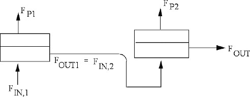
D2. We have a mixture that is 40.0 mol% carbon dioxide and 60.0 mol% oxygen being processed in a perfectly mixed membrane gas permeation separator. A silicone rubber membrane is used at 25.0°C. Permeabilities are PCO2 = 2700 × 10–10 cm3(STP)cm/[cm2·s·cm Hg] and PO2 = 500 × 10–10 cm3(STP)cm/[cm2·s·cm Hg]. Thickness of active layer of membrane is tms = 0.0003 cm. Permeate pressure is pp = 65.0 cm Hg, and retentate pressure is pr = 365 cm Hg. Assume gases are ideal.
a. If we want the highest possible value of permeate mole fraction carbon dioxide, yp, what value of cut θ should be used, what is the value of yp, and what is the value of the retentate mole fraction of carbon dioxide, yr?
b. If we want the lowest possible value of retentate mole fraction carbon dioxide, yr, what value of cut θ should be used, what is the value of yr, and what is the value of permeate mole fraction of carbon dioxide, yp?
D3. We are doing RO experiments with a completely mixed laboratory unit.
Experiment A. With a very high stirrer speed so that there is no concentration polarization, we do an experiment with a feed that is 0.77 wt% sodium chloride in water. Cut θ′ (in mass units) is 0.22, and measured inherent retention is Ro = 0.9804. Permeate pressure is 1.1 atm, T = 40.0°C, and solvent flux is 415.4 g/(m2⋅s). K′solv/tms = 33.29 g/(atm m2⋅s). Data: Assume solutions have the same density as water = 997 kg/m3. Osmotic pressure correlations are given in Eq. (18-14h).
For experiment A, retentate pressure was not recorded. Calculate the value of retentate pressure that was used for this experiment.
D4.* A cellulose acetate membrane is being used for RO of aqueous sucrose solutions at 25.0°C.
Data: Density of solvent (water) is ρ = 0.997 kg/L.
Density (kg/L) of dilute aqueous sucrose solutions is ρ = 0.997 + 0.4x where x is weight fraction sucrose.
At low sucrose weight fraction osmotic pressure (in atm) can be estimated as π = 59.895x where x is the weight fraction sucrose.
Molecular weight of water is 18.016. Molecular weight of sucrose is 342.3.
(Note: Some of this data may not be needed to solve this problem.)
Experiment A. This experiment is done in a well-mixed stirred tank. At 1000.0 rpm with a 3.0 wt% solution of sucrose in water using pr = 75.0 atm and pp = 2.0 atm, we obtain J′solv = 4.625 g/(m2s). Mass transfer coefficient k = 6.94 × 10⁻⁵ m/s. We measure xr = xout = 0.054 and xp = 3.6 × 10⁻⁴.
a. Calculate concentration polarization modulus M.
b. Calculate selectivity α′, K′solv/tms, and K′A/tms.
c. Estimate mass transfer coefficient k if rpm is increased to 2000.0.
D5. We are using a cellulose acetate RO membrane to concentrate a dilute sucrose mixture.
Operation is at 25.0°C.
a. We measure pure water flux (no sucrose present), and find at a pressure drop of 102.0 atm across the membrane J′solv = 1.5 × 10⁻³ [g/(cm2 s)]. An experiment in a highly stirred system (M = 1.0) with a dilute sucrose solution gives a rejection Ro = 0.997 for an inlet weight fraction of 0.050, and cut θ′ = 0.45 (in weight units). Find K′solv/tms and selectivity α′.
b. We will design a perfectly mixed RO system to operate at conditions where M = 3.0. Feed is 2.0 wt% sucrose. We want a cut of θ′ = 2/3. Feed rate will be 5.0 kg/s. Pressure drop across the membrane is 78.0 atm. Plot the RT curve, Eq. (18-20), and find the intersection with the operating line, Eq. (18-23a), to find xp and xr = xout. This is a complete nonlinear (except for linearizing osmotic pressure dependence on sucrose concentration) solution. Then find Jsolv and the membrane area.
c. Resolve part b for xp and xout using linearized solution Eq. (18-29a) with Eqs. (18-25a) and (18-25b).
d. Compare your answer in part c with your answer in part b. Which answer is more accurate?
Data are in Problem 18.D4.
D6. UF of a dextran solution in a well-mixed system with gel formation gives following data:

Determine k and the weight fraction at which dextran gels.
D7. An UF membrane is first tested in a stirred cell in which there is no concentration polarization. Experimental values obtained are listed in the following table. Then the same membrane is used in a spiral-wound module in which there is concentration polarization. Values listed are obtained. Assume membrane thickness and permeabilities are the same. Estimate Roc from stirred-cell data, and assume inherent membrane rejection is unchanged. Calculate expected solvent flux and concentration polarization modulus Mc in the spiral-wound membrane system. No gel layer forms. Use concentration units, g/L. Assume density = 0.997 kg/L.
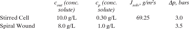
D8. A perfectly mixed membrane module is used to concentrate helium in retentate. Feed is 5.0 vol% helium and 95.0 vol% hydrogen at 5.0 atm. Membrane is natural rubber of the type used by Nakagawa (Table 18-2), and operation is at 25.0°C. The active portion of membrane is 1.0 micron thick. Permeate pressure is 1.0 atm. Assume gases are ideal.
a. If ypHe = 0.025, what are cut θ and yrHe?
b. If θ = 0.75, what are ypHe and yrHe?
c. If yrHe = 0.06, what are cut θ and ypHe?
d. For part a, what membrane area is required for a feed of 100.0 m3(STP)/h?
D9. The following data were obtained for UF of skim milk in a spiral-wound system (Conlee et al., 1998).
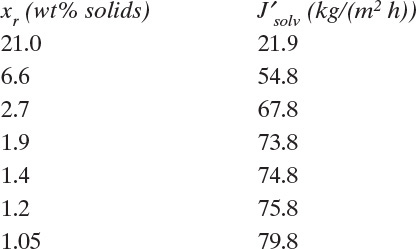
a. Estimate gelling weight fraction, xg, and mass transfer coefficient, k.
b. If you were the technician’s supervisor and one more run could be done, what data would you want the technician to obtain to improve estimate of xg?
D10. We are separating a feed that is 40.0 mol% nitrogen and 60.0 mol% hydrogen in a completely mixed membrane module containing an ethyl cellulose membrane at 30.0°C. Feed rate is 2.0 kmol/min. Permeate cut is θ = 0.20. Membrane thickness is 0.8 µm (0.8 × 10⁻⁴ cm). Permeabilities are in Table 18-2 (Geankoplis data). High pressure is pr = pout = 5.5 atm, and permeate pressure is pp = 1.12 atm. Find:
a. Mole fraction of hydrogen in permeate, yp, and in retentate, yr.
b. Volumetric total flux and volumetric fluxes of hydrogen and nitrogen.
c. Membrane area required, m2.
D11. We are testing a UF membrane in a perfectly stirred system. With pure distilled water we obtain a pure water flux of J = 5000.0 L/(m2 day) at a permeate pressure of 1.0 bar and a retentate pressure of 4.0 bar.
Next we do experiments in the completely mixed system with a constant stirrer speed to separate an aqueous feed that is 0.1 wt% polysaccharide. Previous experiments showed that with this stirred speed, mass transfer coefficient k = 2.89 × 10⁻⁵ m/s. Since the system is quite dilute, solvent density is the same as pure water. Inherent rejection coefficient is Ro = 1.0. Permeate pressure is 1.0 bar, and a cut θ′ (in weight units) of 0.40 is used. Retentate pressure was increased in steps, and the following data were collected:
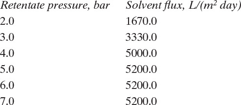
Density of water is 997 kg/m3. Find the weight fraction of polysaccharide at which gelling occurs.
D12. In Example 18-3 we want to increase the nitrogen mole fraction in retentate. To do this we increase retentate pressure to pr = 780.0 mm Hg. Find the value of θ and retentate and permeate mole fractions.
D13. We are running an RO system for an aqueous feed with 3.5 wt% NaCl. This approximates concentration of seawater, but seawater is much more complex. Typically, highest cut for RO of seawater is approximately 0.50 to 0.55. In the United States, EPA lists preferred salt weight fraction in drinking water as 0.00050. In other countries, a higher drinking water maximum salt concentration is used. Operation is at 25.0°C.
a. If xfeed = 0.035, xp = 0.00050, and θ′ = 0.55, what value of retention, R, (including concentration polarization effects) is required?
b. If xfeed = 0.035, xp = 0.00100, and θ′ = 0.55, what value of retention, R, (including concentration polarization effects) is required?
Data: For dilute systems osmotic pressure of sodium chloride is π = a′x where x is weight fraction, π is in atm, and a′ = 705.9 atm/(weight fraction) at 25.0°C. Although this is not a dilute system, to simplify the analysis, assume that the linear equation for osmotic pressure is valid.
D14. A pervaporation system will be used to remove water from n-butanol using a cellulose 2.5-acetate membrane in a perfectly mixed module. Feed is 90.0 mol% n-butanol. Feed rate is 100.0 lb/h. Flux is 0.2 lb/ft2h. Pervaporation unit operates at Tp = Tout = 30.0°C where selectivity of water compared to butanol is 43.0 (in mole fraction units. WATCH UNITS!).
Data: Latent heats: butanol = 141.6 cal/g; water = 9.72 kcal/gmol.
Cp,B (45.0°C) = 0.635 cal/g °C, Cp,w (45.0°C) = 1.0 cal/g °C, MWB = 74.12, MWw = 18.016. Assume heat capacities and latent heats are independent of temperature.
a. If feed is at 60.0°C, find cut, permeate mole fraction, outlet liquid mole fraction, and membrane area.
b. If cut θ = 0.08 is used, find permeate mole fraction, outlet liquid mole fraction, and feed inlet temperature.
c. If outlet water liquid mole fraction is 0.05, find permeate mole fraction, cut, and inlet feed temperature.
D15.* An UF system is concentrating latex particles in an aqueous suspension. System is perfectly mixed on the retentate side and operates with pp = 1.0 bar and pr = 2.2 bar. Because of extensive stirring, concentration polarization modulus is M = 1.2, and no gel forms (xwall < xgel = 0.5). Osmotic pressure of latex particles is negligible. Density of solutions can be assumed to equal density of pure water = 0.997 kg/L. All latex particles are retained by the membrane (Ro = 1.0). Feed to UF module is xr,in = 0.10 weight fraction latex (for all parts). We operate with a cut θ = 0.20. Feed rate of suspension, F′r,in, is 100.0 kg/h. Flux rate of the membrane with pure water is 2500.0 L/(m2 day).
a.* Find F′r,out, xp, and xr,out.
b. What membrane area is required?
c. If we decrease stirring and M increases, at what value of M will gel formation occur (θ′ = 0.20)?
d. At M = 1.2, what value of the cut θ′ will cause gel formation to occur?
e. If M = 1.2 and θ′ = 0.20, at what feed weight fraction will gel formation occur? What is xr,out?
f. We are doing an experiment of slowly decreasing the amount of stirring. If gel formation first occurs with xF = 0.20 and θ′ = 0.25, what are the values of M and mass transfer coefficient k with this amount of stirring? Jsolv = 2500.0, but the area has changed.
g. With the same amount of stirring as in part f but otherwise new conditions, we do an experiment with xF = 0.20, pr = 3.4 bar, pp = 1.0 bar, and θ′ = 0.20. Does a gel form? What is the solvent flux in L/(m2day)?
h. We do an experiment with the same conditions as part g, except θ′ = 0.26. Does a gel form? What is the solvent flux in L/(m2day)?
D16. We are doing RO experiments with a completely mixed laboratory unit. K′solv/tms = 1.387 g/(atm m2s). Data: Assume solutions have same density as water = 997 kg/m3. Osmotic pressure of sodium chloride is π = a′x where x is in weight fraction, π is in atm, and at 25.0°C, a′ = 705.9 atm/(weight fraction).
Experiment B. With a very high stirrer speed so that there is no concentration polarization, we do an experiment with a feed that is 0.077 wt% sodium chloride in water. Cut θ′ (in weight units) is 0.22, and measured inherent retention is Ro = 0.996. pp = 1.1 atm, and pr = 12.06 atm.
Experiment C. A feed with 0.093 wt% sodium chloride was separated with a permeate pressure of 1.1 atm and a retentate pressure of 15.2 atm. Cut (in weight units) θ′ = 0.26. Stirring speed was lower, and concentration polarization is expected. R = 0.992 was measured.
a. What is the value of concentration polarization modulus M in Experiment C?
b. What are the values of xout, xp, and solvent flux J′solv in Experiment C?
D17. On a Robeson (1993) plot (log-log plot of selectivity versus oxygen permeability in Barrer) the upper bound for separation of oxygen from nitrogen plots as a straight line. Approximate values of end points are PO2 = 0.0001 Barrer, αO2–N2 = 42.0; and PO2 = 10,000 Barrer, αO2–N2 = 1.9. Barrer = 10–10 [cc STP cm]/[cm2 s cm Hg].
a. Find the equation for the straight line.
b. If we need an αO2–N2 = 8.0, what is the maximum value of PO2 that can be obtained?
D18. Repeat Example 18-3 except with unknown area and θ = 0.3. Find the value of area, A, and the retentate and permeate mole fractions. Suggestion: Solve with a spreadsheet.
D19. An experiment is being done to determine permanence (permeability/thickness of active layer of membrane), cm3(STP)/[cm2·s·cm Hg], for helium and hydrogen. A perfectly mixed gas permeation unit with 0.20 m2 of area is operated with pr = 13.0 bar and pp = 1.26 bar. With pure He we collect 126.8 cm3(STP)/s. With pure hydrogen we collect 180.1 cm3(STP)/s. Find:
a. Permanence of helium and permanence of hydrogen.
b. Selectivity of H2/He.
c. If tms = 0.0001 cm, calculate PHe and PH2 in cm3(STP)cm/(cm2·s·cm Hg).
D20. A mixture of carbon dioxide, methane, and nitrogen is fed to a perfectly mixed gas permeation system with a natural rubber membrane. Membrane properties are given in Geankoplis data in Table 18-2. Membrane active layer thickness is 1.0 µm. Feed pressure is 17.0 bar = retentate pressure. Permeate pressure is 1.1 bar. Feed is 15.0 mol% carbon dioxide, 75.0 mol% methane, and 10.0 mol% nitrogen. For θ = 0.40 find retentate mole fractions, permeate mole fractions, and membrane area (in m2) needed for 1.0 m3/s of feed gas.
Suggestion: Set up on a spreadsheet or other computer solution method and converge ∑yp – ∑yr = 0 using Goal Seek to change the guessed value of area A.
D21. We are purifying nitrogen by removing oxygen in a gas permeation system. The membrane is a silicone rubber. Thickness of the active layer of the membrane is 0.00007 cm. Feed Fm,1,in = 10.0 kmol/minute and is y1,in = 0.209 mole fraction oxygen. The device has two well-mixed permeation modules coupled in series with retentate from the first module sent as feed to the second. pp = 1.05 atm, and pr = 8.4 atm for both modules. Cut θ1 = 0.4, and we desire yr2,O2 = 0.12 mole fraction O2. Permeability data are in Table 18-2.
Find yr1,O2, yp,1,O2, yp2,O2, θ2, membrane selectivity α, and A2 in m2.
D22. In Example 18-4 we saw that small holes in a membrane are a major problem in gas permeation if high-purity permeate is desired. If we want to produce high-purity water, are holes a problem for RO membranes? One would think answer has to be yes, but let’s calculate and see.
a. We have an RO system producing very pure water (1.0 ppm salt) from a feed that contains 50.0 ppm salt (already purer than normal tap water). If we have one 10.0 µm–diameter pinhole per m2, how much does this affect purity? Conditions: pr = 15.0 bar, pp = 1.1 bar, A = 1.0 m2, K′solv/tms = 0.50 g/(bar·s·m2), cut = θ′ = 0.20, very well mixed: M = 1.0, low concentration: can ignore osmotic pressure.
b. If product water is at 250.0 ppm and the feed is brackish water at 1.0 wt% (10,000 ppm), what is the effect of one 10.0-µm pinhole per m2 on purity? Conditions: pr = 25.0 bar, pp = 1.1 bar, A = 1.0 m2, K′solv/tms = 1.0 g/(bar·s·m2), cut = θ′ = 0.2, very well mixed: M = 1.5, include osmotic pressure. Assume the same density and viscosity as pure water.
Data: Densities of saltwater solution are listed between Eqs. (18-14g) and (18-14h).
Use Eq. (18-14e), (18-14f), or (18-14h) for osmotic pressure. Assume viscosity is 1.0 cp.
D23. UF systems are commonly used for changing solvent or buffer systems when solute is a large molecule such as a protein. Usually the process is operated in a batch mode either in a stirred tank or feed and bleed (Figure 18-2E) but with no bleed of retentate. This process is doing the same function (changing solvents) as batch systems in Section 9.3 but by a totally different mechanism. We have a large solute molecule that is excluded from pores, Rosolute = 1.0. Initial solvent, A, and final solvent, B, are not excluded from pores, RoA = RoB = 0, and have equal fluxes. We want same solute weight fraction in both solvents; thus, if there is initially F kg of solution, at the end of the process we want F kg of solution. Two operating methods are proposed: 1. Dilute a sample with the appropriate amount of solvent B and then do UF to remove excess solvents until you obtain xA,final. 2. Add solvent at the same mass flow rate as the solvents are transferred through the UF membrane.
a. In terms of symbols, how many kg of solvent B are needed to replace F(xA,initial – xA,final) kg of solvent A if on a solute-free basis initial weight fraction of solvent A is xA,initial and final weight fraction of solvent A is xA,final using process 1?
b. In terms of symbols, how many kg of pure solvent B are needed to replace F(xA,initial – xA,final) kg of solvent A if on a solute-free basis initial weight fraction of solvent A is xA,initial and final weight fraction of solvent A is xA,final using process 2?
c. If F = 100.0 kg of A, xr,A,initial = 1.0, and xr,A,final = 0.10, how much solvent is used for each process?
d. If F = 100.0 kg of A, xr,A,initial = 1.0, and xr,A,final = 0.01, how much solvent is used for each process?
D24. For the hybrid system shown in Problem 4.D21, what value of selectivity α is required in a membrane separator to achieve the desired values of yp and yr. Note: This problem does not require solution of Problem 4.D21.
D25. A completely mixed gas permeator is using a 10.0 µm–thick silicone rubber membrane to separate a feed that is 30.0 mol% CO2 and 70.0 mol% CH4 at 25.0°C. High pressure is 20.0 atm, and low pressure is 1.2 atm. Permeabilities are in Table 18-2. Assume gases are ideal.
a. What is the highest possible mole fraction of CO2 in retentate, what is the corresponding CO2 mole fraction in permeate, and what is the value of θ?
b. What is the lowest possible mole fraction of CO2 in retentate, what is the corresponding CO2 mole fraction in permeate, and what is the value of θ?
c. If feed rate is 100.0 m3 STP/s and cut = 0.597, find yr,CO2, yp,CO2, and the membrane area in m2.
D26. A poly (4-methyl pentene) membrane will be used to separate oxygen from nitrogen. Both permeabilities are given in Table 18-2. Thickness of active layer is 0.0002 cm. Feed (and retentate) pressure is 6.1 atm, and permeate pressure is 1.15 atm. Inlet gas is 20.9 mol% oxygen. We desire a permeate mole fraction of yp = 0.42 mole fraction oxygen. Feed rate is Fm,in = 1.2 kmol/min. Assume ideal gases and a well-mixed device. Find the mole fraction of oxygen in retentate = yr, cut θ = Fm,p/Fm,in, and the membrane area, A, in m2.
D27. A mixture of helium, methane, and nitrogen is fed to a perfectly mixed gas permeation system with a silicone rubber membrane. Membrane properties are given in Table 18-2. Membrane active layer thickness is 1.2 µm. Feed pressure is 12.4 bar = retentate pressure. Permeate pressure is 1.1 bar. Feed is 1.6 mol% helium, 87.5 mol% methane, and 10.9 mol% nitrogen. Feed rate is 1.13 m3/s STP.
a. Find retentate mole fractions, permeate mole fractions, and membrane area (in m2) for θ = 0.26.
b. Find retentate mole fractions, permeate mole fractions, and θ for membrane area = 10.0 m2.
D28. We are purifying nitrogen by removing oxygen in a gas permeation system. The membrane is a silicone rubber. Thickness of the active layer of membrane is 0.00011 cm. Feed Fm,1,in = 10.0 kmol/min and is y1,in = 0.21 mole fraction oxygen. The device has two well-mixed permeation modules coupled in series with retentate from the first module sent as feed to the second. pp = 0.8 atm and pr = 6.4 atm for both modules. Fm,p,1 = Fm,p,2 = 2.0 kmol/min. Permeability data are in Table 18-2.
a. Find yr1,O2, yp,1,O2, yr2,O2, yp2,O2, θ2, membrane selectivity α, and areas A1 and A2 in m2.
b. If a single perfectly mixed membrane is separating the same feed with the same conditions except Fm,p = 4.0 kmol/min, calculate yp,O2, yr,O2, yp,O2, θ, and area in m2.
E. More Complex Problems
E1. Your company’s well water, which contains 190.0 ppm (weight) of salt, is fine for most purposes but not for a particular manufacturing process that needs purer water. A vendor is trying to sell you a spiral-wound RO unit that has an inherent salt rejection coefficient of Ro = 0.98, a high pure water flux of J′water = 102.0 g/(m2s) at Δp = 35.0 bar, and approximately 600.0 m2 of area per m3 volume. Modules are available with volumes of 0.5 (300.0 m2), 1.0 (600.0 m2) and 2.0 m3 (1200.0 m2). Modules can be put in parallel or in series. Your company wants to produce 20,000 m3/day of water that contains 12.0 ppm of salt. The retentate, at 480.0 ppm and 1.4 bar, will be used elsewhere in the plant. Inlet pressure of the water is 28.0 bar and cannot be safely increased without a major capital expense. Operation will be at 25.0°C. The sales person wants to do the design for the company (at a price) and will not release his other data. However, he estimates that two large and one medium module will provide the water your company wants.
a. Using available data, estimate the area of the membrane and the operating conditions required to produce the desired permeate and retentate products. Use mass transfer data for spiral-wound systems, but do calculations for a perfectly mixed system.
b. How did the sales person calculate his number?
Data: Typical spiral-wound unit: channels 0.03 to 0.1 cm, velocity = 0.5 to 1.5 m/s, Re = 500.0 to 1000.0 (Wang and Zhou, 2013).
E2. We are doing RO of dilute aqueous sucrose solutions at 25.0°C. A feed that is 2.20 wt% sucrose is separated in a very well-stirred system (M = 1.0) with pr = 60.0 atm and pp = 1.1 atm. The flux J′water = 3.923 g/(m2s) when xp = 0.00032 and xr,out = 0.056. Data are in Problem 18.D4.
a. Calculate cut θ′, inherent rejection Ro, and sucrose flux J′sucrose.
b. Calculate selectivity α′water–sucrose, K′water/tms, K′sucrose/tms, and J′water.
c. If we now repeat the experiment with less mixing so that M = 2.1 with xfeed = 0.0220, pr = 60.0 atm, pp = 1.1 atm, and θ′ = 0.61, calculate xr, xp, J′water, and J′sucrose.
E3. Feed from a distillation column to a pervaporation unit is 90.0 wt% ethanol. After pressurizing and heating to 85.0°C, it is fed to a system similar to Figure 18-14, except retentate can be reheated to 85.0°C and sent to a second pervap stage. Additional stages can be added if needed. A 20.0 micron–thick polyacrylonitrile film membrane is used (see Figure 18-15). Assume each stage of pervap is perfectly mixed and operates at 25.0°C. Final retentate (product) needs to be at 98.5 wt% ethanol or higher. Permeate streams are pressurized and recycled to the distillation column. F = 100.0 kg/h of 90.0 wt% ethanol distillate. Find:
a. Number of stages needed in pervap system.
b. For each stage: cut, permeate flow rate, and product flow rate.
c. Weight fraction of combined permeate streams and retentate weight fraction.
d. Membrane area required for each stage.
F. Problems Requiring Other Resources
F1. A perfectly mixed pervap unit is separating a benzene–isopropyl alcohol mixture. Figure 12-23 in Wankat (1990) shows the separation factor of benzene with respect to isopropyl alcohol versus the weight fraction of benzene in liquid for pervap. If operation is at 50.0°C = Tp = Tout, xin = 30.0 wt% benzene and the θ = 0.10, find yp, xout, and Tin. Assume heat capacities and latent heats are independent of temperature.
Note: Use lines on the selectivity diagram, not data points.
H. Spreadsheet Problems
H1. A spreadsheet or other computer method (e.g., MATLAB, Mathmatica) is required. Repeat Problem 18.D10 except for a crossflow system. Report the average yp, yr, membrane area, volumetric total flux, and volumetric fluxes of hydrogen and nitrogen. Turn in a copy of your spreadsheet or other program with numbers for both parts a and b.
a. Find the solution for N = 1, which is the perfectly mixed answer.
b. Find the solution for N = 1000, which is the crossflow answer.
H2.* In Section 18.3.3 the following statement appears, “Geankoplis (2003) solves the multicomponent permeator system by a different method, but the results are identical.” Solve Example 13.5-1 in Geankoplis (2003) using the method in Section 18.3.3 with a spreadsheet, and show that the results agree with Geankoplis’ solution.
H3. Pervaporation problems are trial and error but can be conveniently solved on a spreadsheet if selectivity is constant. Solve Problem 18.D14a with a spreadsheet, and check your answer with graphical solution. Graphical and spreadsheet solutions should agree.
H4. Repeat Problem 18.D14a but with the feed at 80.0°C.
H5. RO experiments are done in a laboratory stirred-tank membrane system at 45.0°C. With pure water we measure the pure water flux = 17.89 g/(m2 s) when pr = 15.2 atm and pp = 1.1 atm. We then do experiment A with a highly stirred system (M = 1.0) with pr = 13.4 atm and pp = 1.1 atm and find Ro = 0.991. We now plan on doing an experiment with pr = 11.3 atm and pp = 1.1 atm, θ′ = 0.55, xin =0.03 wt% salt, and a mass transfer coefficient of k = 4.63 × 10⁻⁵ m/s. Density of water is 0.997 kg/L. Predict M, R, J′solv, xp, and xr for the new experiment. Use of a spreadsheet or other computer solver is highly recommended.
H6. Repeat Problem 18.H5 except with xin = 0.0006, and find the value of k that gives M = 1.1. Report k, R, J′solv, xp, and xr. Use of a spreadsheet or other computer solver is highly recommended.
H7. Repeat Problem 18.H5 (xin = 0.003) but with pr = 21.4 atm and pp = 1.1 atm, θ′ = 0.45, and a mass transfer coefficient of k = 4.63 × 10⁻⁵ m/s. Predict M, R, J′solv, xp, and xr for the new experiment.
Introduction to Design Problems 18.H8 and 18.H9
Find the configuration with the lowest total annual cost for the separation assigned to your team.
Estimate the total annual cost (TAC) as
Although there are other costs (e.g., capital cost for heat exchangers to cool gas after compression and energy cost for cooling water), include only the following three costs:
1. Capital cost for membrane systems
2. Capital cost for compressors
3. Electricity cost for operation of compressors
Use electricity cost as $0.06/kWh. 8760 h/yr.
Compressor hp requirements use the Quick chart from www.agcsi.com/estimate/chart1A1.htm, which is based on compressing natural gas. The chart gives the horsepower required to compress 1.0 million cubic feet per day at the inlet condition (not STP).
Centrifugal compressor costs with motor including installation factor and cost index (Woods, 2007).
Base 1000.0 kW. $1.592 × 10⁶, Cost at x kW = cost 1000 kW(x kW/1000 kW)n, n = 0.9 for 2000 to 4000 kW.
Base 10,000 kW. $12.2 × 10⁶, Cost x kW = cost 10,000 kW(x kW/10,000 kW)n, n = 0.71 for 8000 to 25,000 kW.
Membrane module, not including compressor: cost including installation factor and cost index (Woods, 2007): Base 560.0 m2, $153,000. Cost at x m2 = cost at 560.0 m2(x m2/560.0)n, n = 1.0 for 560.0 to 10,000 m2.
If required areas are larger, put modules in parallel. Assume ideal gases.
Design group report requirements are listed in Chapter 11 in the introduction to Problems 11.G6 to 11.G9.
H8. Helium is in short supply worldwide. There are natural gas sources that contain large amounts of low-concentration helium. Your job is to develop a membrane cascade using spiral-wound membrane permeators, which are essentially crossflow systems, to produce 1.0 m3STP product/min of a 90.0 mol% or slightly higher helium product from a feed that is 1.0 mol% He and 99.0 mol% CH4. Use membrane properties in Table 18-2. Feed gas is at 25.0°C and 25.0 atm. In a real design you can pick any retentate pressures you want, but you have to pay for compression. You could also pick any permeate pressure you want for each module. To simplify the problem use a retentate pressure of 25.0 atm and a permeate pressure of 1.1 atm for all membranes. Active layer is tms = 3.0 µm. Assume the supply of natural gas is larger than you need. Methane depleted of helium will be sent back to the pipeline at 25.0 atm. Assume costs of compressing retentate to pipeline pressure is negligible. Helium product needs to be compressed to 25.0 atm. Report feed rate, membrane area, yp,avg, yr, and θ for each membrane module in your cascade. Include a sketch of your cascade.
H9. A natural gas field produces a gas that is 30.0 mol% carbon dioxide and 70.0 mol% methane. Design crossflow separators that will process 100.0 m3 STP/s of fresh feed. Use Table 18-2 for permeability data. Membrane is in a spiral-wound system and is 10.0 µm thick. Feed pressure is 20.0 atm, and permeate pressure is 1.2 atm. Use a constant permeate pressure of 1.2 atm. You can vary retentate pressure. The methane and carbon dioxide products will be delivered at 20.0 atm.
a. If we use a cross-flow system with a silicone rubber membrane at 25.0°C find the value of cut θ that produces a retentate with CO2 mole fraction = 0.10 or slightly less. Report membrane area, yp,avg, yr, and θ. Then, set N = 1, find yr at same value of θ (yr will be > 0.1), and check your answer for a perfectly mixed membrane system with a hand solution of problem 18.D25c. The purpose is to benchmark the spreadsheet program.
b. If we use a cross-flow system with a ethyl cellulose membrane at 30.0°C find the value of cut that produces a retentate with CO2 mole fraction = 0.10 or slightly less. Report membrane area, yp,avg, yr, and θ.
c. The membrane in part a is high flux but relatively low selectivity. In part b the membrane is higher selectivity but lower flux. What are the advantages and the disadvantages of each membrane?
d. Determine the most economical cross-flow system (based on lowest value of TAC) using one or more modules to obtain a methane product that has CO2 mole fraction = 0.10 or slightly less with a methane yield of 80.0% (or more). Include a sketch of your membrane cascade. Report membrane type, membrane area, yp,avg, yr, and θ for each membrane module in the cascade.
Chapter 18 Appendix. Spreadsheet for Crossflow Gas Permeation
Flow pattern calculations can be done with an Excel spreadsheet using Visual Basic for Applications (VBA). The spreadsheet and VBA program are for a constant value of selectivity, α, although it would not be difficult to use an α that depended on gas mole fraction. This program is an example of spreadsheet programs to analyze the three flow configurations shown in Figure 18-19. If you only want to see effects of changing variables, you can use this spreadsheet as a semiblack box and not touch the VBA program. If you are unfamiliar with using a spreadsheet that includes a VBA macro, read Appendix 4B, Part 1. If you want to learn VBA programming, an effective approach is to modify the program in Table 18-A1.
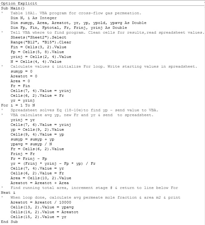
Crossflow calculation requires no trial and error and is fast even with N = 1000, which is the recommended value. Data is input on the spreadsheet, which also calculates yp,stage j from Eq. (18-10e) and Astage j from Eq. (18-66). These values are transferred to the VBA program, which calculates yr,j, Fr,j, yp,total, and Atotal and increments the stage number. The spreadsheet with equations is shown in Figure 18-A1 and with results for Example 18-12 in Figure 18-A2. The VBA program is shown in Table 18-A1.
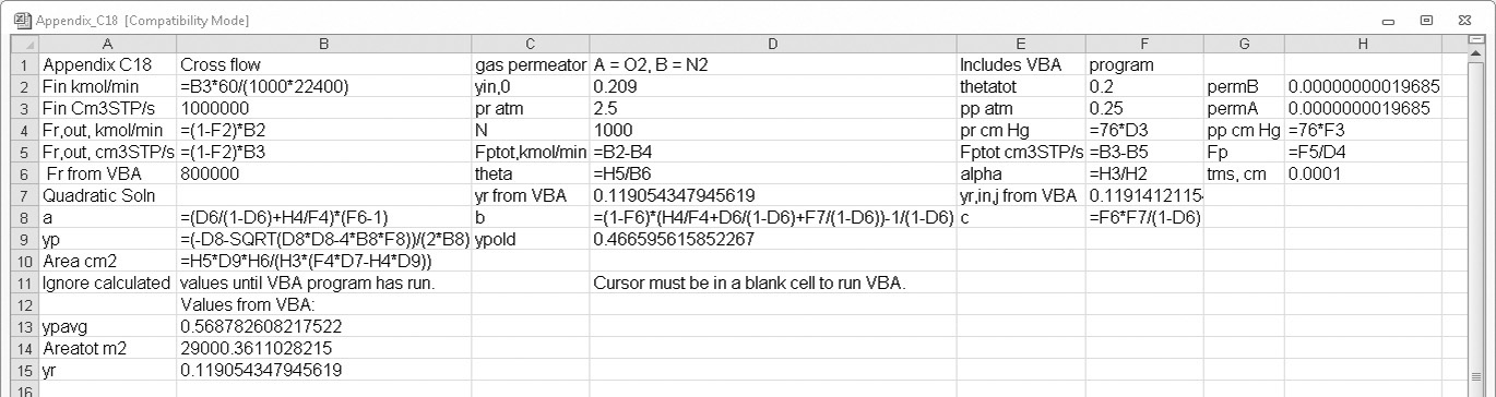
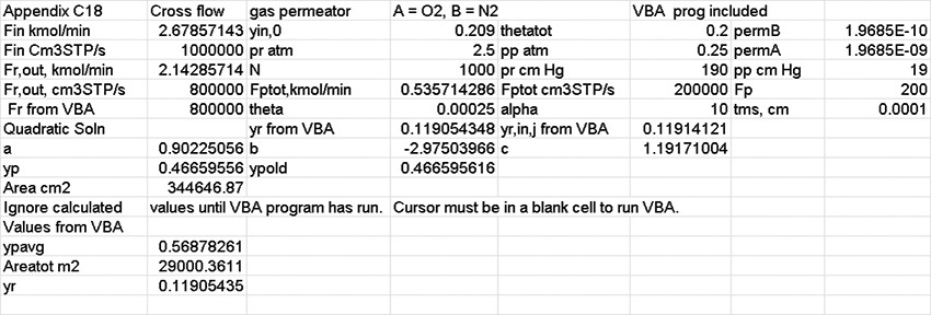
Although splitting calculations between a spreadsheet and the VBA program has advantages, it is important to ensure correct values of parameters that change as the stage number is incremented are used to calculate yp and area. Equations (18-10c) and (18-10d) show that yp is calculated with the inlet value of yr (yr,j–1 labeled yrinj in VBA) and the value of θ from Eq. (18-64c). Area is calculated with yp,j and xr,j. Since spreadsheets update values immediately, whereas VBA programs update values sequentially in the For loop, if you are not careful, there can be a mismatch in update timing.