
6. Sales Force and Channel Management
Introduction
This chapter deals with push marketing. It describes how marketers measure the adequacy and effectiveness of the systems that provide customers with reasons and opportunities to buy their products.
The first sections discuss sales force metrics. Here, we list and define the most common measures for determining whether sales force effort and geographic coverage are adequate. We discuss pipeline analysis, which is useful in making sales forecasts and in allocating sales force effort to different stages of the selling process. Pipeline metrics are used to examine a sequence of selling activities, from lead generation, through follow-up, to conversion and sales. Although the most important of these represents the percentage of initial leads who ultimately buy, other measures of activity, productivity, efficiency, and cost can be useful at each stage of the selling process.
In further sections of this chapter, we discuss measures of product distribution and availability. For manufacturers who approach their market through resellers, three key metrics provide an indication of “listings”—the percentage of potential outlets that stock their products. These include numeric distribution, which is unweighted; ACV, the industry standard; and PCV, a category-specific measure of product availability.
Marketing logistics tracking metrics are used to measure the operational effectiveness of the systems that service retailers and distributors. Inventory turns, out-of-stocks, and service levels are key factors in this area.
At the retail level, gross margin return on inventory investment (GMROII) and direct product profitability (DPP) offer SKU-specific metrics of product performance, combining movement rates, gross margins, costs of inventory, and other factors.
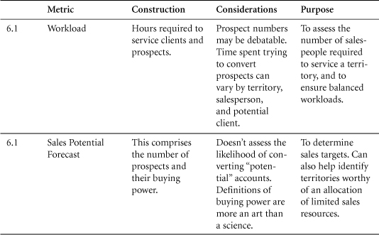

6.1 Sales Force Coverage: Territories
Workload (#) = [Current Accounts (#) * Average Time to Service an Active Account (#)] + [Prospects (#) * Time Spent Trying to Convert a Prospect into an Active Account (#)]
Sales Potential ($) = Number of Possible Accounts (#) * Buying Power ($)
Purpose: To create balanced sales territories.
There are a number of ways to analyze territories.1 Most commonly, territories are compared on the basis of their potential or size. This is an important exercise. If territories differ sharply or slip out of balance, sales personnel may be given too much or too little work. This can lead to under- or over-servicing of customers.
When sales personnel are stretched too thin, the result can be an under-servicing of customers. This can cost a firm business because over-taxed salespeople engage in sub-optimal levels of activity in a number of areas. They seek out too few leads, identify too few prospects, and spend too little time with current customers. Those customers, in turn, may take their business to alternate providers.
Over-servicing, by contrast, may raise costs and prices and therefore indirectly reduce sales. Over-servicing in some territories may also lead to under-servicing in others.
Unbalanced territories also raise the problem of unfair distribution of sales potential among members of a sales force. This may result in distorted compensation and cause talented salespeople to leave a company, seeking superior balance and compensation.
Achieving an appropriate balance among territories is an important factor in maintaining satisfaction among customers, salespeople, and the company as a whole.
Construction
In defining or redefining territories, companies strive to
• Balance workloads
• Balance sales potential
• Develop compact territories
• Minimize disruptions during the redesign
These goals can have different effects on different stakeholders, as represented in Table 6.1.2
Before designing new territories, a sales force manager should evaluate the workloads of all members of the sales team. The workload for a territory can be calculated as follows:
Workload (#) = [Current Accounts (#) * Average Time to Service an Active Account (#)] + [Prospects (#) * Time Spent Trying to Convert a Prospect into an Active Account (#)]
The sales potential in a territory can be determined as follows:
Sales Potential ($) = Number of Possible Accounts (#) * Buying Power ($)
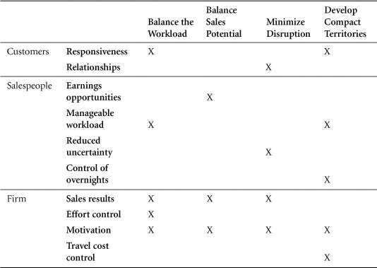
Table 6.1 Effects of Balancing Sales Territories
Buying power is a dollar figure based on such factors as average income levels, number of businesses in a territory, average sales of those businesses, and population demographics. Buying power indices are generally specific to individual industries.
In addition to workload and sales potential, a third key metric is needed to compare territories. This is size or, more specifically, travel time. In this context, travel time is more useful than size because it more accurately represents the factor that size implies—that is, the amount of time needed to reach customers and potential customers.
As a manager’s goal is to balance workload and potential among sales personnel, it can be beneficial to calculate combined metrics—such as sales potential or travel time—in order to make comparisons between territories.
Data Sources, Complications, and Cautions
Sales potential can be represented in a number of ways. Of these, the most basic is population—the number of potential accounts in a territory. In the copier case cited earlier, this might be the number of offices in a territory.
Estimating the size of a territory might involve simply calculating the geographic area that it covers. It is likely, however, that average travel time will also be important. Depending on the quality of roads, density of traffic, or distance between businesses, one may find that territories of equal area entail very different travel time requirements. In evaluating such distinctions, sales force records of the time needed to travel from call to call can be useful. Specialized computer software programs are available for these purposes.
Redefining territories is a famously difficult process. To perform it well, in addition to the metrics cited earlier, disruption of customer relationships and feelings of ownership among sales personnel must also be considered.
6.2 Sales Force Objectives: Setting Goals
Many of these approaches involve a combination of historical results and a weighting of sales potential among the territories. This ensures that overall goals will be attained if all salespeople meet their individual goals.
Purpose: To motivate sales personnel and establish benchmarks for evaluating and rewarding their performance.
In setting sales goals, managers strive to motivate their personnel to stretch themselves and generate the most sales possible. But they don’t want to set the bar too high. The correct goal levels will motivate all salespeople and reward most of them.
When planning sales goals, certain guidelines are important. Under the SMART strategy recommended by Jack D. Wilner, author of Seven Secrets to Successful Sales Management,3 goals should be Specific, Measurable, Attainable, Realistic, and Timebound. Goals should be specific to a department, a territory, and even a salesperson. They should be clear and applicable to each individual so that salespeople do not have to derive part of their goal. Measurable goals, expressed in concrete numbers such as “dollar sales” or “percentage increase,” enable salespeople to set precise targets and track their progress. Vague goals, such as “more” or “increased” sales, are not effective because they make it difficult to measure progress. Attainable goals are in the realm of possibility. They can be visualized and understood by both the manager and the salesperson. Realistic goals are set high enough to motivate, but not so high that salespeople give up before they even start. Finally, time-bound goals must be met within a precise time frame. This applies pressure to reach them sooner rather than later and defines an endpoint when results will be checked.
Construction
There are numerous ways of allotting a company’s forecast across its sales force. These methods are designed to set goals that are fair, achievable, and in line with historic results. Goals are stated in terms of sales totals for individual salespeople. In the following formulas, which encapsulate these methods, a district is composed of the individual territories of multiple salespeople.
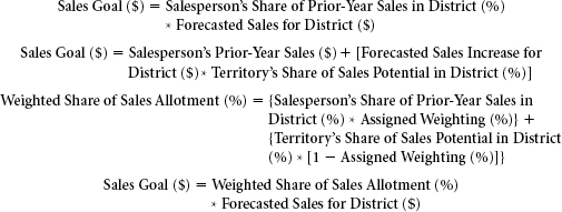
A sales goal or allocation based on prior-year sales can be calculated as follows:4
Sales Goal ($) = Salesperson’s Share of Prior-Year Sales in District (%) * Forecasted Sales for District ($)
A sales goal based on prior-year sales and the sales potential of a territory can be calculated as follows:
Sales Goal ($) = Salesperson’s Prior-Year Sales ($) + [Forecasted Sales Increase for District($) * Territory’s Share of Sales Potential in District (%)]
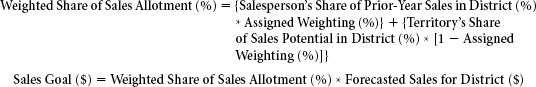
Sales goals can also be set by a combined method, in which management assigns weightings to both the prior-year sales of each salesperson and the sales potential of each territory. These weightings are then used to calculate each salesperson’s percentage share of the relevant sales forecast, and percentage shares are used to calculate sales goals in dollar terms.
Data Sources, Complications, and Cautions
Sales goals are generally established by using combinations of bottom-up and top-down procedures. Frequently, top management sets objectives at a corporate level, while the sales manager allocates shares of that overall goal among the various members of the sales force.
Top management generally uses multiple metrics to forecast sales, including prior-year sales of the product in question, total prior-year sales in the relevant market, prior-year sales by competitors, and the company’s current market share. After the corporate sales forecast is derived, a sales force manager verifies that these targets are reasonable, pushing back where necessary. The manager then allots the projected sales among the sales force in a district, based at least in part on measures of individual performance from the prior year. Of greatest importance in this calculation are each salesperson’s historic percentage of sales and the sales potential of his or her territory.
It is important to re-evaluate sales goals during the year to ensure that actual performance is running reasonably close to projections. If, at this checkpoint, it appears that more than 90% or less than 50% of the sales force is on track to achieve their goals, then it may be advisable to alter the goals. This will prevent salespeople from easing off too early because their goals are in sight, or giving up because their goals are unattainable. In setting goals, one possible rule of thumb would be to plan for a success rate of 75%. That would ensure that enough salespeople reach their goal and that the goal is sufficiently challenging.
If “rebudgeting” becomes necessary, it is important to ensure that this is properly recorded. Unless care is taken, revised sales goals can slip out of alignment with financial budgets and the expectations of senior management.
6.3 Sales Force Effectiveness: Measuring Effort, Potential, and Results

Each can also be calculated on a dollar contribution basis.
Purpose: To measure the performance of a sales force and of individual salespeople.
When analyzing the performance of a salesperson, a number of metrics can be compared. These can reveal more about the salesperson than can be gauged by his or her total sales.
Construction
An authoritative source lists the following ratios as useful in assessing the relative effectiveness of sales personnel:5
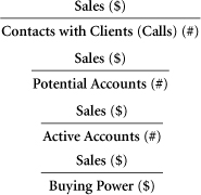
These formulas can be useful for comparing salespeople from different territories and for examining trends over time. They can reveal distinctions that can be obscured by total sales results, particularly in districts where territories vary in size, in number of potential accounts, or in buying power.
These ratios provide insight into the factors behind sales performance. If an individual’s sales per call ratio is low, for example, that may indicate that the salesperson in question needs training in moving customers toward larger purchases. Or it may indicate a lack of closing skills. If the sales per potential account or sales per buying power metric is low, the salesperson may not be doing enough to seek out new accounts. These metrics reveal much about prospecting and lead generation because they’re based on each salesperson’s entire territory, including potential as well as current customers. The sales per active account metric provides a useful indicator of a salesperson’s effectiveness in maximizing the value of existing customers.
Although it is important to make the most of every call, a salesperson will not reach his or her goal in just one call. A certain amount of effort is required to complete sales. This can be represented graphically (see Figure 6.1).6
Although one can increase sales by expending more time and attention on a customer, at a certain point, a salesperson encounters diminishing returns in placing more calls to the same customers. Eventually, the incremental business generated by each call will be worth less than the cost of making the call.
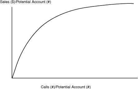
Figure 6.1 Sales Resulting from Calls to Customers
In addition to the formulas described earlier, one other important measure of effectiveness is the ratio of expenses to sales. This cost metric is commonly expressed as a percentage of sales and is calculated as follows:
If this ratio is substantially higher for one salesperson than for others, it may indicate that the individual in question has poor control of his or her expenses. Examples of poor expense control could include making unnecessary trips to a client, overproducing product pamphlets, or hosting too many dinners. Alternatively, expenses may represent a high percentage of sales if an individual possesses poor closing skills. If a salesperson’s expenses are comparable to those of his peers, but his sales are lower, then he may be failing to deliver sales after spending significant money on a potential customer.
A more challenging set of sales force performance metrics involves customer service. Customer service is difficult to measure because there are no concrete numbers representing it, other than repeat rates or customer complaints. Each of those is telling, but how can a sales manager evaluate the service provided to customers who are not repeating, leaving, or complaining? One possibility is to develop a survey, including an itemized scale to help customers quantify their opinions. After enough of these surveys are completed, managers will be able to calculate average scores for different service metrics. By comparing these with sales figures, managers can correlate sales with customer service and grade salespeople on their performance.
EXAMPLE: To translate customers’ opinions into a metric, a company might pose survey questions such as the following:
Please circle the level of service your business received from our sales staff after shipment of the products you ordered:
Data Sources, Complications, and Cautions
Calculating the effectiveness of a salesperson is not difficult, but it does require keeping track of a few important numbers. Fortunately, these are commonly recorded in the sales industry.
The most important statistics are the amount of each sale (in dollars) and the contribution generated by that sale. It may also be important to keep track of which items are sold if a salesperson has been instructed to emphasize a certain product line. Additional useful information would include measures of the number of calls made (including both face-to-face and phone meetings), total accounts active, and total accounts in the territory. Of these, the latter two are needed to calculate the buying power of a territory.
The largest problem in performance review is a tendency to rely on only one or two metrics. This can be dangerous because an individual’s performance on any one measure may be anomalous. A salesperson who generates $30,000 per call may be more valuable than one who generates $50,000 per call, for example, if he generates greater sales per potential account. A salesperson in a small territory may generate low total contribution but high dollar sales per buying power. If this is true, it may be advisable to increase the size of that person’s territory. Another salesperson may show a dramatic increase in dollar sales per active account. If he achieves this simply by eliminating weaker accounts without generating incremental sales, it would not be grounds for reward. In reviewing sales personnel, managers are advised to evaluate as many performance metrics as possible.
Although the customer service survey described earlier is grounded upon a straightforward concept, managers can find it difficult to gather enough data—or sufficiently representative data—to make it useful. This could be because customers hesitate to fill out the surveys, or because they do so only when they encounter a problem. A small sample size or a prevalence of negative responses might distort the results. Even so, some effort to measure customer satisfaction is needed to ensure that salespeople don’t emphasize the wrong issues—or neglect issues that have a substantial impact on customers’ lifetime value.
6.4 Sales Force Compensation: Salary/Reward Mix
Purpose: To determine the mix of salary, bonus, and commission that will maximize sales generated by the sales force.
When designing a compensation plan for a sales force, managers face four key considerations: level of pay, mix between salary and incentive, measures of performance, and performance-payout relationships. The level of pay, or compensation, is the amount that a company plans to pay a salesperson over the course of a year. This can be viewed as a range because its total will vary with bonuses or commissions.
The mix between salary and incentive represents a key allocation within total compensation. Salary is a guaranteed sum of money. Incentives can take multiple forms, including bonuses or commissions. In the case of a bonus, a salesperson will receive a lump sum for reaching certain sales targets. With a commission, the incentive is incremental and is earned on each sale. In order to generate incentives, it is important to measure accurately the role a salesperson plays in each sale. The higher the level of causality that can be attributed to a salesperson, the easier it is to use an incentive system.
Various metrics can be used to measure a salesperson’s performance. With these, managers can evaluate a salesperson’s performance in the context of past, present, or future comparators, as follows:
• The past: Measure the salesperson’s percentage growth in sales over prior-year results.
• The present: Rank salespeople on the basis of current results.
• The future: Measure the percentage of individual sales goals achieved by each salesperson.
Sales managers can also select the organizational level on which to focus an incentive plan. The disbursement of incentive rewards can be linked to results at the company, division, or product-line level. In measuring performance and designing compensation plans along all these dimensions, managers seek to align salespeople’s incentives with the goals of their firm.
Lastly, a time period should be defined for measuring the performance of each salesperson.
Construction
Managers enjoy considerable freedom in designing compensation systems. The key is to start with a forecast for sales and a range within which each salesperson’s compensation should reside. After these elements are determined, there are many ways to motivate a salesperson.
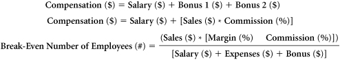
In a multi-bonus system, the following formula can represent the compensation structure for a salesperson:
Compensation ($) = Salary ($) + Bonus 1 ($) + Bonus 2 ($)
In this system, bonus 1 might be attained at a level approximately halfway to the individual’s sales goal for the year. The second bonus might be awarded when that goal is met.
In a commission system, the following formula would represent compensation for a salesperson:
Compensation ($) = Salary ($) + [Sales ($) * Commission (%)]
Theoretically, in a 100% commission structure, salary might be set as low as $0. Many jurisdictions, however, place limits on such arrangements. Managers must ensure that their chosen compensation structures comply with employment law.
Managers can also combine bonus and commission structures by awarding bonuses on top of commissions at certain sales levels, or by increasing the commission rate at certain sales levels.
EXAMPLE: Tina earns a commission of 2% on sales up to $1,000,000, and a 3% commission on sales beyond that point. Her salary is $20,000 per year. If she makes $1,200,000 in sales, her compensation can be calculated as follows:
After a sales compensation plan has been established, management may want to re-evaluate the size of its sales force. Based on forecasts for the coming year, a firm may have room to hire more salespeople, or it may need to reduce the size of the sales force. On the basis of a given value for projected sales, managers can determine the break-even number of employees for a firm as follows:
Data Sources, Complications, and Cautions
Measurements commonly used in incentive plans include total sales, total contribution, market share, customer retention, and customer complaints. Because such a plan rewards a salesperson for reaching certain goals, these targets must be defined at the beginning of the year (or other time period). Continual tracking of these metrics will help both the salesperson and the company to plan for year-end compensation.
Timing is an important issue in incentive plans. A firm must collect data in a timely fashion so that both managers and salespeople know where they stand in relation to established goals. The time frame covered by a plan also represents an important consideration. If a company tries to generate incentives through weekly rewards, its compensation program can become too expensive and time-consuming to maintain. By contrast, if the program covers too long a period, it may slip out of alignment with company forecasts and goals. This could result in a sales force being paid too much or too little. To guard against these pitfalls, managers can develop a program that mixes both short- and long-term incentives. They can link some rewards to a simple, short-term metric, such as calls per week, and others to a more complex, long-term target, such as market share achieved in a year.
A further complication that can arise in incentive programs is the assignment of causality to individual salespeople. This can become a problem in a number of instances, including team collaborations in landing sales. In such a scenario, it can be difficult to determine which team members deserve which rewards. Consequently, managers may find it best to reward all members of the team with equal bonuses for meeting a goal.
A last concern: When an incentive program is implemented, it may reward the “wrong” salespeople. To avoid this, before activating any newly proposed program, sales managers are advised to apply that program to the prior year’s results as a test. A “good” plan will usually reward the salespeople whom the manager knows to be the best.
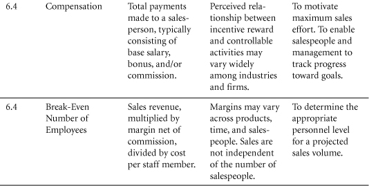
6.5 Sales Force Tracking: Pipeline Analysis
Purpose: To forecast upcoming sales and evaluate workload distribution.
A convenient way to forecast sales in the short term and to keep an eye on sales force activity is to create a sales pipeline or sales funnel. Although this concept can be represented graphically, the data behind it are stored electronically in a database or spreadsheet.
The concept of the sales funnel originates in a well-known dynamic: If a sales force approaches a large number of potential customers, only a subset of these will actually make purchases. As salespeople proceed through multiple stages of customer interaction, a number of prospects are winnowed out. At the conclusion of each stage, fewer potential customers remain. By keeping track of the number of potential customers at each stage of the process, a sales force manager can balance the workload within a team and make accurate forecasts of sales.
This analysis is similar to the hierarchy of effects discussed in Section 2.7. Whereas the hierarchy of effects focuses on the impact of advertising or mass media, the sales funnel is used to track individual customers (often by name) and sales force efforts. (Note: In some industries, such as consumer packaged goods, the term “pipeline sales” can refer to sales into a distribution channel. Please do not confuse pipeline sales with a sales pipeline.)
Construction
In order to conceptualize a sales funnel or pipeline, it is helpful to draw a diagram showing the stages of the selling process (see Figure 6.2). At any point in the year, it is likely that all stages of the pipeline will include some number of customers. As Figure 6.2 illustrates, although there may be a large number of potential customers, those who actually make purchases represent only a percentage of these original leads.

Figure 6.2 Sales Force Funnel
Interest Creation: This entails building awareness of a product through such activities as trade shows, direct mail, and advertising. In the course of interest creation, salespeople can also generate leads. That is, they can identify targets to add to their pool of potential customers. Two main classifications of leads include cold leads and warm leads.
Cold Lead: A lead that has not specifically expressed interest. These can be identified through mailing lists, phone books, business listings, and so on.
Warm Lead: A lead that is expected to be responsive. These potential customers may have registered through a Web site or requested product information, for example.
Pre-Purchase: This stage involves identifying prospects from among cold and warm leads. Salespeople make this distinction through initial meetings with leads, in which they explain product features and benefits, and cooperate in problem solving with the customer. The desired result of such an early-stage meeting is not a sale but rather the identification of a prospect and the scheduling of another meeting.
Prospect: A potential customer who has been identified as a likely buyer, possessing the ability and willingness to buy.8
Purchase: After prospects are identified and agree to additional calls, salespeople engage in second and third meetings with them. It is in these sessions that traditional “selling” takes place. Salespeople will engage in persuading, negotiating, and/or bidding. If a purchase is agreed upon, a salesperson can close the deal through a written proposal, contract, or order.
Post-Purchase: After a customer has made a purchase, there is still considerable work to be done. This includes delivery of the product or service, installation (if necessary), collection of payments, and possibly training. There is then an ongoing commitment to customer service.
After salespeople visualize the different stages represented in a sales funnel, they can track their customers and accounts more accurately. They can do this electronically by using a database or spreadsheet. If a sales pipeline file is maintained on a shared drive, any member of a sales force will be able to update the relevant data on a regular basis. This will also enable a sales manager to view the progress of the team at any point in time. Table 6.2 is an example of a spreadsheet form of a sales funnel.
A manager can use the information stored in such a funnel to prepare for sales in the near future. This is a form of pipeline analysis. When a firm faces inventory issues, or when sales goals are being missed, this represents vital information. By applying historical averages, a sales or marketing manager can improve sales forecasts by using the data in a sales funnel. This can be done manually or with specialized software. The underlying assumption behind a sales funnel is that failure at any stage eliminates a prospect from the funnel. The following example illustrates how this bottom-up forecasting could be applied.
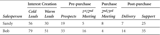
Table 6.2 Spreadsheet Sales Funnel
Data Sources, Complications, and Cautions
In order to populate a sales funnel correctly, salespeople must maintain records of all their current and potential customers, and the status of each within the purchase process. Each salesperson must also share this information, which can then be aggregated in a comprehensive database of sales force activities. By applying assumptions to these—including assumptions drawn from historical sales results—a firm can project future sales. For example, if 25% of warm leads are generally converted to sales within two months, and 200 warm leads currently appear in a sales funnel, management can estimate that 50 of these will be converted to sales within two months.
At times, the use of a sales funnel leads to the pitfall of over-prospecting. If the incremental contribution generated by a customer is less than the cost of acquiring that customer, then prospecting for that customer yields a negative result. Salespeople are advised to use customer lifetime value metrics as a guide in deciding the appropriate scale and direction of their prospecting. Increasing pre-purchase sales funnel metrics will not be worthwhile unless that increment leads to improved figures further down the pipeline as well.
Difficulties in the sales cycle can also arise when a salesperson judges that a potential customer may be a prospect because he or she has the willingness and ability to buy. To solidify this judgment, the salesperson must also confirm that the customer possesses the authority to buy. When prospecting, salespeople should take the time needed to verify that their contacts can make purchase decisions without approval from another source.
6.6 Numeric, ACV and PCV Distribution, Facings/Share of Shelf
For marketers who sell through resellers, distribution metrics reveal a brand’s percentage of market access. Balancing a firm’s efforts in “push” (building and maintaining reseller and distributor support) and “pull” (generating customer demand) is an ongoing strategic concern for marketers.
Purpose: To measure a firm’s ability to convey a product to its customers.
In broad terms, marketing can be divided into two key challenges:
• The first—and most widely appreciated—is to ensure that consumers or end users want a firm’s product. This is generally termed pull marketing.
• The second challenge is less broadly recognized, but often just as important. Push marketing ensures that customers are given opportunities to buy.
Marketers have developed numerous metrics by which to judge the effectiveness of the distribution system that helps create opportunities to buy. The most fundamental of these are measures of product availability.
Availability metrics are used to quantify the number of outlets reached by a product, the fraction of the relevant market served by those outlets, and the percentage of total sales volume in all categories held by the outlets that carry the product.
Construction
There are three popular measures of distribution coverage:
1. Numeric distribution
2. All commodity volume (ACV)
3. Product category volume (PCV), also known as weighted distribution
Numeric Distribution
This measure is based on the number of outlets that carry a product (that is, outlets that list at least one of the product’s stock-keeping units, or SKUs). It is defined as the percentage of stores that stock a given brand or SKU, within the universe of stores in the relevant market.
The main use of numeric distribution is to understand how many physical locations stock a product or brand. This has implications for delivery systems and for the cost of servicing these outlets.
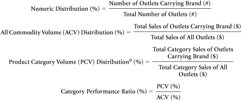
Numeric Distribution: To calculate numeric distribution, marketers divide the number of stores that stock at least one SKU of a product or brand by the number of outlets in the relevant market.
For further information about stock-keeping units (SKUs), refer to Section 3.3.
All Commodity Volume
All commodity volume (ACV) is a weighted measure of product availability, or distribution, based on total store sales. ACV can be expressed as a dollar value or percentage.
All Commodity Volume (ACV): The percentage of sales in all categories that are generated by the stores that stock a given brand (again, at least one SKU of that brand).

EXAMPLE: The marketers at Madre’s Tortillas want to know the all commodity volume of their distribution network (Table 6.3).
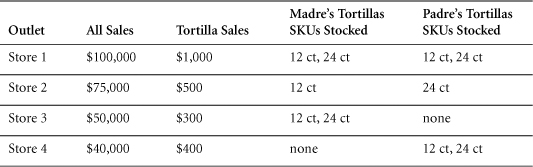
Table 6.3 Madre’s Tortillas’ Distribution
Madre’s Tortillas are carried by Stores 1-3, but not by Store 4. The ACV of its distribution network is therefore the total sales of Stores 1, 2, and 3, divided by the total sales of all stores. This represents a measure of the sales of all commodities in these stores, not just tortilla sales.
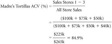
The principal benefit of the ACV metric, by comparison with numeric distribution, is that it provides a superior measure of customer traffic in the stores that stock a brand. In essence, ACV adjusts numeric distribution for the fact that not all retailers generate the same level of sales. For example, in a market composed of two small stores, one superstore, and one kiosk, numeric distribution would weight each outlet equally, whereas ACV would place greater emphasis on the value of gaining distribution in the superstore. In calculating ACV when detailed sales data are not available, marketers sometimes use the square footage of stores as an approximation of their total sales volume.
The weakness of ACV is that it does not provide direct information about how well each store merchandises and competes in the relevant product category. A store can do a great deal of general business but sell very little of the product category under consideration.
Product Category Volume
Product category volume (PCV)10 is a refinement of ACV. It examines the share of the relevant product category sold by the stores in which a given product has gained distribution. It helps marketers understand whether a given product is gaining distribution in outlets where customers look for its category, as opposed to simply high-traffic stores where that product may get lost in the aisles.
Continuing our example of the two small retailers, the kiosk, and the superstore, although ACV may lead the marketer of a chocolate bar to seek distribution in the high-traffic superstore, PCV might reveal that the kiosk, surprisingly, generates the greatest volume in snack sales. In building distribution, the marketer would then be advised to target the kiosk as her highest priority.
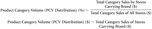
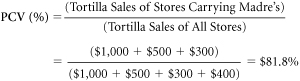
Product Category Volume (PCV): The percentage share, or dollar value, of category sales made by stores that stock at least one SKU of the brand in question, in comparison with all stores in their universe.
When detailed sales data are available, PCV can provide a strong indication of the market share within a category to which a given brand has access. If sales data are not available, marketers can calculate an approximate PCV by using square footage devoted to the relevant category as an indication of the importance of that category to a particular outlet or store type.
EXAMPLE: The marketers at Madre’s Tortillas want to know how effectively their product is reaching the outlets where customers shop for tortillas. Using data from the previous example:
Stores 1, 2, and 3 stock Madre’s Tortillas. Store 4 does not. The product category volume of Madre’s Tortillas’ distribution network can be calculated by dividing total tortilla sales in Stores 1-3 by tortilla sales throughout the market.
Total Distribution: The sum of ACV or PCV distribution for all of a brand’s stock-keeping units, calculated individually. By contrast with simple ACV or PCV, which are based on the all commodity or product-category sales of all stores that carry at least one SKU of a brand, total distribution also reflects the number of SKUs of the brand that is carried by those stores.
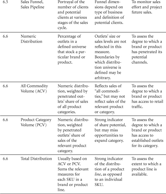
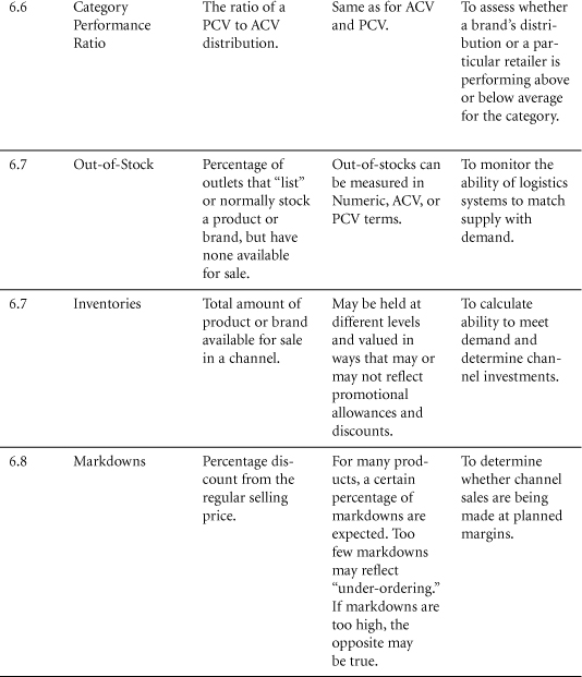
Category Performance Ratio: The relative performance of a retailer in a given product category, compared with its performance in all product categories.
By comparing PCV with ACV, the category performance ratio provides insight into whether a brand’s distribution network is more or less effective in selling the category of which that brand is a part, compared with its average effectiveness in selling all categories in which members of that network compete.
If a distribution network’s category performance ratio is greater than 1, then the outlets comprising that network perform comparatively better in selling the category in question than in selling other categories, relative to the market as a whole.
Data Sources, Complications, and Cautions
In many markets, there are data suppliers such as A.C. Nielsen, which specialize in collecting information about distribution. In other markets, firms must generate their own data. Sales force reports and shipment invoices provide a place to start.
For certain merchandise—especially low-volume, high-value items—it is relatively simple to count the limited number of outlets that carry a given product. For higher-volume, lower-cost goods, merely determining the number of outlets that stock an item can be a challenge and may require assumptions. Take, for instance, the number of outlets selling a specific soft drink. To arrive at an accurate number, one would have to include vending machines and street vendors as well as traditional grocery stores.
Total outlet sales are often approximated by quantifying selling space (measured in square feet or square meters) and applying this measure to industry averages for sales per area of selling space.
In the absence of specific category sales data, it is often useful to weight ACV to arrive at an approximation of PCV. Marketers may know, for example, that pharmacies, relative to their overall sales, sell proportionally more of a given product than do superstores. In this event, they might increase the weighting of pharmacies relative to superstores in evaluating relevant distribution coverage.
Related Metrics and Concepts
Facing: A facing is a frontal view of a single package of a product on a fully stocked shelf.
Share of Shelf: A metric that compares the facings of a given brand to the total facing positions available, in order to quantify the display prominence of that brand.
Store Versus Brand Measures: Marketers often refer to a grocery chain’s ACV. This can be either a dollar number (the chain’s total sales of all categories in the relevant geographic market) or a percentage number (its share of dollar sales among the universe of stores). A brand’s ACV is simply the sum of the ACVs of the chains and stores that stock that brand. Thus, if a brand is stocked by two chains in a market, and these chains have 40% and 30% ACV respectively, then the ACV of that brand’s distribution network is 30% + 40%, or 70%.
Marketers can also refer to a chain’s market share in a specific category. This is equivalent to the chain’s PCV (%). A brand’s PCV, by contrast, represents the sum of the PCVs of the chains that stock that brand.
Inventory: This is the level of physical stock held. It will typically be measured at different points in a pipeline. A retailer may have inventory on order from suppliers, at warehouses, in transit to stores, in the stores’ backrooms, and on the store shelves.
Breadth of Distribution: This figure can be measured by the number of SKUs held. Typically, a company will hold a wide range of SKUs—a high breadth of distribution—for the products that it is most interested in selling.
Features in Store: The percentage of stores offering a promotion in a given time period. This can be weighted by product or by all commodity volume (ACV).
ACV on Display: Distinctions can be made in all commodity volume metrics to take account of where products are on display. This will reduce the measured distribution of products if they are not in a position to be sold.
AVC on Promotion: Marketers may want to measure the ACV of outlets where a given product is on promotion. This is a useful shorthand way of determining the product’s reliance on promotion.
6.7 Supply Chain Metrics
Logistics tracking helps ensure that companies are meeting demand efficiently and effectively.
Purpose: To monitor the effectiveness of an organization in managing the distribution and logistics process.
Logistics are where the marketing rubber meets the road. A lot can be lost at the potential point-of-purchase if the right goods are not delivered to the appropriate outlets on time and in amounts that correspond to consumer demand. How hard can that be? Well, ensuring that supply meets demand becomes more difficult when:
• The company sells more than a few stock keeping units (SKUs).
• Multiple levels of suppliers, warehouses, and stores are involved in the distribution process.
• Product models change frequently.
• The channel offers customer-friendly return policies.
In this complex field, by monitoring core metrics and comparing these with historical norms and guidelines, marketers can determine how well their distribution channel is functioning as a supply chain for their customers.
By monitoring logistics, managers can investigate questions such as the following: Did we lose sales because the wrong items were shipped to a store that was running a promotion? Are we being forced to pay for the disposal of obsolete goods that stayed too long in warehouses or stores?
Construction
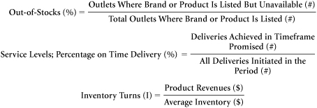
Out-of-Stocks: This metric quantifies the number of retail outlets where an item is expected to be available for customers, but is not. It is typically expressed as a percentage of stores that list the relevant item.
Being “listed” by a chain means that a headquarters buyer has “authorized” distribution of a brand, SKU, or product at the store level. For various reasons, being listed does not always ensure presence on the shelf. Local managers may not approve “distribution.” Alternatively, a product may be distributed but sold out.
Out-of-stocks are often expressed as a percentage. Marketers must note whether an out-of-stock percentage is based on numeric distribution, ACV, PCV, or the percentage of distributing stores for a given chain.
The in-stock percentage is the complement of the out-of-stock percentage. A 3% out-of-stock rate would be equivalent to a 97% in-stock rate.
PCV Net Out-of-Stocks: The PCV of a given product’s distribution network, adjusted for out-of-stock situations.
Product Category Volume (PCV), Net Out-of-Stocks: This out-of-stocks measure is calculated by multiplying PCV by a factor that adjusts it to recognize out-of-stock situations. The adjusting factor is simply one minus the out-of-stocks figure.
Product Category Volume, Net Out-of-Stocks (%) = PCV (%) * [1 – Out-of-Stock (%)]
Service Levels, Percentage On-time Delivery: There are various service measures in marketing logistics. One particularly common measure is on-time delivery. This metric captures the percentage of customer (or trade) orders that are delivered in accordance with the promised schedule.
Inventories, like out-of-stocks and service levels, should be tracked at the SKU level. For example, in monitoring inventory, an apparel retailer will need to know not only the brand and design of goods carried, but also their size. Simply knowing that there are 30 pairs of suede hiking boots in a store, for example, is not sufficient—particularly if all those boots are the same size and fail to fit most customers.
By tracking inventory, marketers can determine the percentage of goods at each stage of the logistical process—in the warehouse, in transit to stores, or on the retail floor, for example. The significance of this information will depend on a firm’s resource management strategy. Some firms seek to hold the bulk of their inventory at the warehouse level, for example, particularly if they have an effective transport system to ship goods quickly to stores.
Inventory Turns: The number of times that inventory “turns over” in a year can be calculated on the basis of the revenues associated with a product and the level of inventory held. One need only divide the revenues associated with the product in question by the average level of inventory for that item. As this quotient rises, it indicates that inventory of the item is moving more quickly through the process. Inventory turns can be calculated for companies, brands, or SKUs and at any level in the distribution chain, but they are frequently most relevant for individual trade customers. Important note: In calculating inventory turns, dollar figures for both sales and inventory must be stated either on a cost or wholesale basis, or on a retail or resale basis, but the two bases must not be mixed.
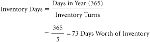
Inventory Days: This metric also sheds light on the speed with which inventory moves through the sales process. To calculate it, marketers divide the 365 days of the year by the number of inventory turns, yielding the average number of days of inventory carried by a firm. By way of example, if a firm’s inventory of a product “turned” 36.5 times in a year, that firm would, on average, hold 10 days’ worth of inventory of the product. High inventory turns—and, by corollary, low inventory days—tend to increase profitability through efficient use of a firm’s investment in inventory. But they can also lead to higher out-of-stocks and lost sales.
Inventory days represents the number of days’ worth of sales that can be supplied by the inventory present at a given moment. Viewed from a slightly different perspective, this figure advises logistics managers of the time expected to elapse before they suffer a stock-out. To calculate this figure, managers divide product revenue for the year by the value of the inventory days, generating expected annual turns for that inventory level. This can be easily converted into days by using the previous equation.
EXAMPLE: An apparel retailer holds $600,000 worth of socks in inventory January 1, and $800,000 the following December 31. Revenues generated by sock sales totaled $3.5 million during the year.
To estimate average sock inventory during the year, managers might take the average of the beginning and ending numbers: ($600,000 + $800,000)/2 = $700,000 average inventory. On this basis, managers might calculate inventory turns as follows:

If inventory turns five times per year, this figure can be converted to inventory days in order to measure the average number of days worth of stock held during the period.
Data Sources, Complications, and Cautions
Although some companies and supply chains maintain sophisticated inventory tracking systems, others must estimate logistical metrics on the basis of less-than-perfect data. Increasingly, manufacturers may also have difficulty purchasing research because retailers that gather such information tend to restrict access or charge high fees for it. Often, the only readily available data may be drawn from incomplete store audits or reports filed by an overloaded sales force. Ideally, marketers would like to have reliable metrics for the following:
• Inventory units and monetary value of each SKU at each level of the distribution chain for each major customer.
• Out-of-stocks for each SKU, measured at both the supplier and the storelevel.
• Percentage of customer orders that were delivered on time and in the correct amount.
• Inventory counts in the tracking system that don’t match the number in the physical inventory. (This would facilitate a measure of shrinkage or theft.)
When considering the monetary value of inventory, it is important to use comparable figures in all calculations. As an example of the inconsistency and confusion that can arise in this area, a company might value its stock on the retail shelf at the cost to the store, which might include an approximation of all direct costs. Or it might value that stock for some purposes at the retail price. Such figures can be difficult to reconcile with the cost of goods purchased at the warehouse and can also be different from accounting figures adjusted for obsolescence.
When evaluating inventory, managers must also establish a costing system for items that can’t be tracked on an individual basis. Such systems include the following:
• First In, First Out (FIFO): The first unit of inventory received is the first expensed upon sale.
• Last In, First Out (LIFO): The last unit of inventory received is the first expensed upon sale.
The choice of FIFO or LIFO can have a significant financial impact in inflationary times. At such times, FIFO will hold down the cost of goods sold by reporting this figure at the earliest available prices. Simultaneously, it will value inventory at its highest possible level—that is, at the most recent prices. The financial impact of LIFO will be the reverse.
In some industries, inventory management is a core skill. Examples include the apparel industry, in which retailers must ensure that they are not left with prior seasons’ fashions, and the technology industry, in which rapid developments make products hard to sell after only a few months.
In logistical management, firms must beware of creating reward structures that lead to sub-optimal outcomes. An inventory manager rewarded solely for minimizing out-of-stocks, for example, would have a clear incentive to overbuy—regardless of inventory holding costs. In this field, managers must ensure that incentive systems are sophisticated enough not to reward undesirable behavior.
Firms must also be realistic about what will be achieved in inventory management. In most organizations, the only way to be completely in stock on every product all the time is to ramp up inventories. This will involve huge warehousing costs. It will tie up a great deal of the company’s capital in buying stocks. And it will result in painful obsolescence charges to unload over-purchased items. Good logistics and inventory management entails finding the right trade-off between two conflicting objectives: minimizing both inventory holding costs and sales lost due to out-of-stocks.
Related Metrics and Concepts
Rain Checks, or Make-Goods on Promotions: These measures evaluate the effect on a store of promotional items being unavailable. In a typical example, a store might track the incidents in which it offers customers a substitute item because it has run out of stock on a promoted item. Rain checks or make-goods might be expressed as a percentage of goods sold, or more specifically, as a percentage of revenues coded to the promotion but generated by sales of items not listed as part of the promotional event.
Misshipments: This measures the number of shipments that failed arrive on time or in the proper quantities.
Deductions: This measures the value of deductions from customer invoices caused by incorrect or incomplete shipments, damaged goods, returns, or other factors. It is often useful to distinguish between the reasons for deductions.
Obsolescence: This is a vital metric for many retailers, especially those involved in fashion and technology. It is typically expressed as the monetary value of items that are obsolete, or as the percentage of total stock value that comprises obsolete items. If obsolescence is high, then a firm holds a significant amount of inventory that is likely to sell only at a considerable discount.
Shrinkage: This is generally a euphemism for theft. It describes a phenomenon in which the value of actual inventory runs lower than recorded inventory, due to an unexplained reduction in the number of units held. This measure is typically calculated as a monetary figure or as a percentage of total stock value.
Pipeline Sales: Sales that are required to supply retail and wholesale channels with sufficient inventory to make a product available for sale (refer to Section 6.5).
Consumer Off-Take: Purchases by consumers from retailers, as opposed to purchases by retailers or wholesalers from their suppliers. When consumer off-take runs higher than manufacturer sales rates, inventories will be drawn down.
Diverted Merchandise or Diverted Goods: Products shipped to one customer that are subsequently resold to another customer. For example, if a retail drug chain overbuys vitamins at a promotional price, it may ship some of its excess inventory to a dollar store.
6.8 SKU Profitability: Markdowns, GMROII, and DPP
By monitoring markdowns, marketers can gain important insight into SKU profitability. GMROII can be a vital metric in determining whether sales rates justify inventory positions. DPP is a theoretically powerful measure of profit that has fallen out of favor, but it may be revived in other forms (for example, activity-based costing).
Purpose: To assess the effectiveness and profitability of individual product and category sales.
Retailers and distributors have a great deal of choice regarding which products to stock and which to discontinue as they make room for a steady stream of new offerings. By measuring the profitability of individual stock keeping units (SKUs), managers develop the insight needed to optimize such product selections. Profitability metrics are also useful in decisions regarding pricing, display, and promotional campaigns.
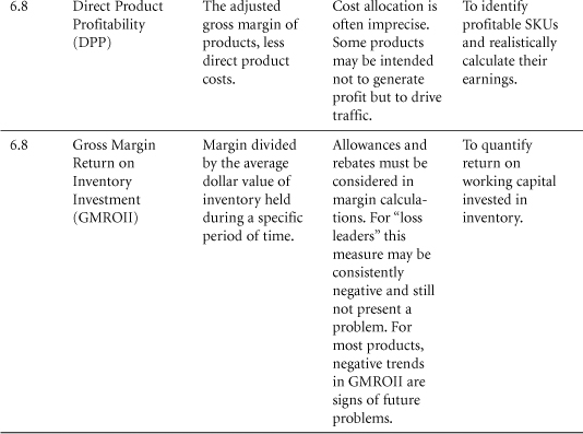
Figures that affect or reflect retail profitability include markdowns, gross margin return on inventory investment, and direct product profitability. Taking each in turn:
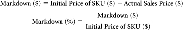
Markdowns are not always applied to slow-moving merchandise. Markdowns in excess of budget, however, are almost always regarded as indicators of errors in product assortment, pricing, or promotion. Markdowns are often expressed as a percentage of regular price. As a standalone metric, a markdown is difficult to interpret.
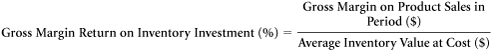
Gross margin return on inventory investment (GMROII) applies the concept of return on investment (ROI) to what is often the most crucial element of a retailer’s working capital: its inventory.
Direct product profitability (DPP) shares many features with activity-based costing (ABC). Under ABC, a wide range of costs are weighted and allocated to specific products through cost drivers—the factors that cause the costs to be incurred. In measuring DPP, retailers factor such line items as storage, handling, manufacturer’s allowances, warranties, and financing plans into calculations of earnings on specific product sales.
Construction
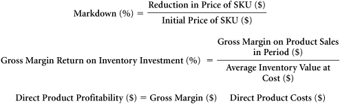
Markdown: This metric quantifies shop-floor reductions in the price of a SKU. It can be expressed on a per-unit basis or as a total for the SKU. It can also be calculated in dollar terms or as a percentage of the item’s initial price.
Gross Margin Return on Inventory Investment (GMROII): This metric quantifies the profitability of products in relation to the inventory investment required to make them available. It is calculated by dividing the gross margin on product sales by the cost of the relevant inventory.
Direct Product Profitability (DPP)
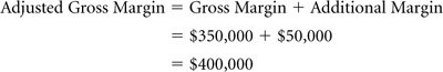
Direct product profitability is grounded in a simple concept, but it can be difficult to measure in practice. The calculation of DPP consists of multiple stages. The first stage is to determine the gross margin of the goods in question. This gross margin figure is then modified to take account of other revenues associated with the product, such as promotional rebates from suppliers or payments from financing companies that gain business on its sale. The adjusted gross margin is then reduced by an allocation of direct product costs, described next.
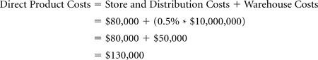
Direct Product Costs: These are the costs of bringing a product to customers. They generally include warehouse, distribution, and store costs.
Direct Product Costs ($) = Warehouse Direct Costs ($) + Transportation Direct Costs ($) + Store Direct Costs ($)
Direct Product Profitability (DPP): Direct product profitability represents a product’s adjusted gross margin, less its direct product costs.
As noted earlier, the concept of DPP is quite simple. Difficulties can arise, however, in calculating or estimating the relevant costs. Typically, an elaborate ABC system is needed to generate direct costs for individual SKUs. DPP has fallen somewhat out of favor as a result of these difficulties.
Other metrics have been developed, however, in an effort to obtain a more refined and accurate estimation of the “true” profitability of individual SKUs, factoring in the varying costs of receiving, storing, and selling them. The variations between products in the levels of these costs can be quite significant. In the grocery industry, for example, the cost of warehousing and shelving frozen foods is far greater—per unit or per dollar of sales—than the cost of warehousing and shelving canned goods.
Direct Product Profitability ($) = Gross Margin ($) – Direct Product Costs ($)
EXAMPLE: The apparel retailer cited earlier wants to probe further into the profitability of its sock line. Toward that end, it assembles the following information. For this retailer, socks generate slotting allowances—in essence, fees paid by the manufacturer to the retailer in compensation for shelf space—in the amount of $50,000 per year. Warehouse costs for the retailer come to $10,000,000 per year. Socks consume 0.5% of warehouse space. Estimated store and distribution costs associated with socks total $80,000.
With this information, the retailer calculates an adjusted gross margin for its sock line.
The retailer then calculates direct product costs for its sock line.
On this basis, the retailer calculates the direct product profitability of its sock line.
Data Sources, Complications, and Cautions
For GMROII calculations, it is necessary to determine the value of inventory held, at cost. Ideally, this will be an average figure for the period to be considered. The average of inventory held at the beginning and end of the period is often used as a proxy, and is generally—but not always—an acceptable approximation. To perform the GMROII calculation, it is also necessary to calculate a gross margin figure.
One of the central considerations in evaluating direct product profitability is an organization’s ability to capture large amounts of accurate data for analysis. The DPP calculation requires an estimate of the warehousing, distribution, store direct, and other costs attributable to a product. To assemble these data, it may be necessary to gather all distribution costs and apportion them according to the cost drivers identified.
Inventory held, and thus the cost of holding it, can change considerably over time. Although one may usually approximate average inventory over a period by averaging the beginning and ending levels of this line item, this will not always be the case. Seasonal factors may perturb these figures. Also, a firm may hold substantially more—or less—inventory during the course of a year than at its beginning and end. This could have a major impact on any DPP calculation.
DPP also requires a measure of the ancillary revenues tied to product sales.
Direct product profitability has great conceptual strength. It tries to account for the wide range of costs that retailers incur in conveying a product to customers, and thus to yield a more realistic measure of the profitability of that product. The only significant weakness in this metric is its complexity. Few retailers have been able to implement it. Many firms continue to try to realize its underlying concept, however, through such programs as activity-based costing.
Related Metrics and Concepts
Shopping Basket Margin: The profit margin on an entire retail transaction, which may include a number of products. This aggregate transaction is termed the “basket” of purchases that a consumer makes.
One key factor in a firm’s profitability is its capability to sell ancillary products in addition to its central offering. In some businesses, more profit can be generated through accessories than through the core product. Beverage and snack sales at movie theaters are a prime example. With this in mind, marketers must understand each product’s role within their firm’s aggregate offering—be it a vehicle to generate customer traffic, or to increase the size of each customer’s basket, or to maximize earnings on that item itself.
References and Suggested Further Reading
Wilner, J.D. (1998). 7 Secrets to Successful Sales Management: The Sales Manager’s Manual, Boca Raton: St. Lucie Press.
Zoltners, A.A., P. Sinha, and G.A. Zoltners. (2001). The Complete Guide to Accelerating Sales Force Performance, New York: Amacom.