
12. System of Metrics
“There are three kinds of economists: those who can count and those who can’t.”—Unknown source
Modeling Firm Performance
To better understand the factors contributing to overall firm success, managers and analysts often decompose return on assets (ROA) into the product of two ratios with each ratio reflecting a different aspect of the business. One popular approach or “model” for this decomposition is the DuPont Model.
The first ratio in this simplified DuPont Model is called either the profit margin or return on sales. It measures how profitable is each dollar of sales. To the extent that marketers create products that customers value, claim that value through intelligent pricing, drive down costs by paying attention to manufacturing and channel costs, and optimize their marketing spending, marketers can increase the firm’s return on sales. The second ratio in the DuPont Model is known as asset turnover. Asset turnover can be thought of as the number of dollars of sales each dollar of assets generates. Here the job of marketers is even more focused—on generating dollars of sales but with an eye toward managing assets such as inventory and receivables captured in the denominator.
Notice that the DuPont Model is an identity.1 It is always true regardless of the values taken on by the various ratios. It is always true mostly because we have defined the ratios in such a way so as to make it always true. So it makes no sense to argue with or take exception to the DuPont Model.
But if it is simply an equation that is true by definition, what good is it? It is useful to the extent that the decomposition of ROA into the two component ratios helps firms maximize ROA by focusing (separately) on the two components. It is also useful in that it reminds marketers that their job is not simply to generate sales, but to generate profitable sales and to do so efficiently (with respect to assets used).
The DuPont Model has demonstrated its usefulness in practice. A Google search resulted in 4.4 million results for “DuPont Model” compared to 2.9 million results for “DuPont Chemicals.” In some circles, the company is now more famous for its model than its chemicals.
Figure 12.1 illustrates how the DuPont Model is often expanded to include components affecting the two input ratios.
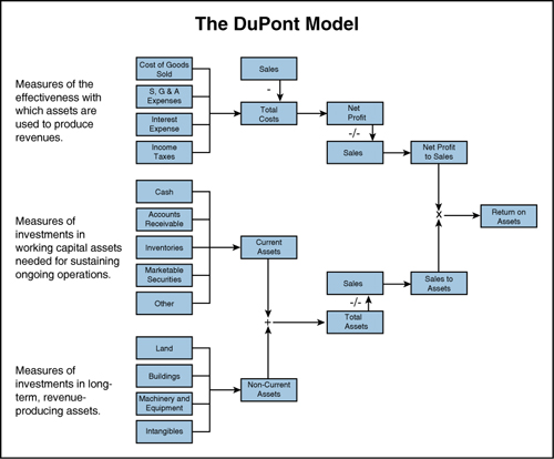
Figure 12.1 An Extended DuPont Model (adapted from http://www.12manage.com/methods_dupont_model.html)
Notice that the three rightmost columns of boxes in Figure 12.1 represent the DuPont Model. The two leftmost columns of boxes represent a particular method of breaking apart net profit and total assets into smaller components. Our purpose here is not to critique the above representation of the components of firm performance, but simply to offer a few observations. First, we note that the decompositions of total costs, current assets, and non-current assets should be familiar to most readers. The categories of components used are consistent with what one finds on income statements (where total cost appears) and balance sheets (where total assets appears). Second, we note that the assets that marketing creates (brands and customer relationships, for example) get lumped together as intangibles signaling that they are difficult to measure (which we agree with) and perhaps an afterthought or “other” category (which we disagree with).
Finally, and most importantly, we observe that although total cost, current assets, and non-current assets all get broken out into smaller, well-understood components, sales does not. It is as if Costs and Assets deserve a lot of attention but the components of sales do not. This is perhaps not surprising since this particular model was designed by finance and accounting executives. As marketers, however, much of our focus is on how sales are generated. We also care about costs and asset utilization, of course, but we care more about sales and the components of sales. Figure 12.1 reflects the inward focus of a firm whose success depended on making things, minimizing costs, and using assets efficiently. For today’s firms whose success depends at least as much on marketing and sales as production, we need a different model. We need our own “DuPont Model,” with at least the same amount of detail and clarity for breaking down the components of sales as the commonly used breakdowns of costs and assets.
Of course, as we begin to think about how to break down sales into its components, we quickly come to understand why there is no commonly used breakdown across different types of businesses. As all marketers know, there are multiple ways to decompose or break down sales simply because several entities (most of them outside the firm) are involved in the creation of revenue: sales force, customers, dealers, and even our competition. With a multitude of insightful ways to break down sales, it is no wonder there is not one commonly accepted way.
To illustrate, Figure 12.2 shows four (of many) separate and valid ways to break down sales into smaller components.
• SALES = Number Salespersons * Avg. Sales/Salesperson
• SALES = Number dealers ACV% * Avg. Sales per dealer ACV%
• SALES = Our Dollar Share * Total Market Sales
• SALES = Number customers * Sales per customer
As with the DuPont Model, each of four ways to compute sales is an identity. Sales will always equal the number of customers times the average sales per customer. But even though they are identities, they can still lead to valuable insights as we will attempt to demonstrate.
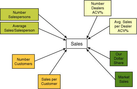
We also point out that there will be other ways to break down sales. Figure 12.2 simply illustrates four ways. Also know that the outer ring of components of sales in Figure 12.2 can themselves be decomposed. For example: Sales per customer can be calculated as Purchases per customer (per period) * Average Sales per purchase. And, not unexpectedly, there will be multiple ways to decompose each of the outer-ring components. For example Sales per customer can also be decomposed into Units purchased per customer * Average price per unit. Decomposing the components of sales can be thought of as expanding the diagram in Figure 12.2 outward. We might also think of expanding the model “upward” with separate pages (decompositions) for each product or each customer group or each vendor.
Three Reasons for Using Systems of Identities in Marketing
There are three primary reasons for formulating marketing DuPont-like component models of your marketing decisions and objectives:
1. Decomposing the metric of interest into components can make it possible to identify problems and opportunities for improvement in more detail. For example, did share drop because our sales were down or competitors’ sales were up? If our sales were down, was that due to fewer customers buying, lower unit sales per customer, lower average prices, or some combination? Decomposition may also help by separating identities from empirical relationships. Although identities are easy (just arithmetic), empirical relationships require difficult judgments about the form of the relationship, causality, and the future.
2. Decomposing metrics may also allow us to estimate, indirectly, other component metrics that are difficult to measure directly. Using multiple identities can help eliminate measurement error with multiple “checks” on the value of any specific metrics. In the same way, individual marketing metrics may be regarded as part of a network or “web” of relationships. If each link in the network is valid, even if individual values are estimated with error, the entire structure will be more robust.
3. Selecting and organizing the right network of marketing metrics often helps formulate models of marketing mix decisions. Like the DuPont Model, using models with interim components can make such models and dashboards more managerially transparent and help managers make and monitor the effects of their decisions.
Decomposing for Diagnostic Purposes
As mentioned previously, a primary purpose for using one or more identities to decompose any marketing metric of interest is to gain a deeper understanding (or at least a different perspective) on the reasons for changes and differences observed. Although identities may be developed with a view to understanding the sources of changes and differences, they do not require calibration or estimation. They are true by definition, and we will designate these with an (ID).
An example of an identity is the relationship between Sales, Quantity, and Price:
Sales = Quantity × Price (ID)
This identity tells us that Sales declines whenever quantity decreases (as a percentage) more than price increases. If we witness declining sales, the identity helps us see, first, whether the decline was due to declining quantity or price or both. And next it helps us understand that if quantity declined, price increased, but sales declined, that quantity must have declined by a larger percentage than did the price increase.
In contrast to identities are empirical relationships—relationships between variables for which the exact equation is not known and/or for which the relationship holds only imperfectly. Empirical relationships are required, for example, to help us decide whether we should increase or decrease prices. We designate these with an (EM). For example, we might consider the relationship between quantity sold to be a direct, linear function of price charged:
Quantity = b × Price + error (EM)
This empirical relationship between quantity and price necessarily contains an error to account for measuring price or quantity imperfectly or influences on quantity sold other than price (our competitors’ prices, for example). Also note that the parameter “b” in this empirical relationship is, itself, a variable. It is an unknown constant—one that we might, for example, be able to estimate from available data. But one of the key differences between identities (ID) and empirical relationships (EM) is that empirical relationships are more flexible. They apply to the tough and important questions such as “how many more units will we sell if we lower the price by $1?”
Dashboards of metrics often reflect underlying management logic about how marketing works to influence sales and profits. Dashboards include both identities and empirical relationships. As illustrated in Figure 12.2, sales can be decomposed many ways. Some of the components of sales might themselves be decomposed using one or more identities. Each firm needs to identify its primary performance measures. This is what should appear on their dashboards. There should be the capability to drill down on each of these performance measures (using identities) to diagnose and explain changes across time. But if dashboards are to be more than monitoring devices, we should have some idea of causal connections (step on the brake to slow down the vehicle, step on the accelerator to make it go faster). Before long, they can become complicated as we start to take into consideration the multiple effects of some of the variables, e.g., step on the accelerator to make the car go faster and the fuel gauge drops. Sometimes we also need a system of metrics to help infer (or forecast) values that are difficult to measure directly (e.g., how much farther can we drive before the gas tank is empty?).
Eliminating Error by Harnessing the Law of Large (and Not So Large) Numbers
There is the classic story of the physics professor whose final exam asked students to explain how to use a barometer to measure the height of a building. In addition to the “obvious” answer to measure the barometric pressures at the top and bottom of the building and use the difference to calculate the building’s height, the professor purportedly received several other creative answers. Drop the barometer from the top of the building, time how long it takes to hit the ground, and use the appropriate physics formula to infer the height. Tie the barometer to a string, lower it to the ground, and measure the length of the string. Measure the length of the shadow cast by the building, the length of the shadow cast by the barometer, the height of the barometer, and use proportions to calculate the height of the building. By far the most creative solution purportedly offered was to knock on the door of the building’s janitor and offer to give the janitor the barometer in exchange for revealing the height of the building.
The multiple ways to calculate sales shown in Figure 12.2 are similar to the multiple ways students came up with to measure the height of the building. Rather than argue over which single method to use, we propose to look for a way to use them all. When faced with a dilemma of which of two methods to use, why not do both? For the barometer problem, why not use several different methods and then combine the many estimates into one final estimate—perhaps by doing something as simple as taking the average of the estimates. If we wanted to do a little bit better, we could calculate a weighted average with weights depending on some measure of how “accurate” each estimate was. We might put more weight on the string-based estimate and less on the estimate from timing the fall of the barometer if we thought our watch and wind made the timing-based estimate less accurate. The relative weight to put on the janitor’s estimate would depend on our confidence in the estimate. If the janitor claims to “know” the height, we should give the estimate more weight than if the janitor admits the number is something of a guess.
Using the average of the estimates instead of any one of the estimates takes advantage of the law of large (and not so large) numbers. The average is expected to be closer to the true value and become closer the more estimates that we have to average together. Ideally we want “independent” estimates such as might be the case with the barometer example (unless, of course, the janitor got his number using the string method).
In the barometer example, we were mostly interested in measuring the height of the building. In our example, marketers are probably just as interested in the measuring components as we are in measuring sales itself. In fact, it often is the case that the firm has a good handle on sales and would like to get a better measure of some of the components such as share or the sales per customer or any of the other metrics in the outer ring or outer-outer ring. In extreme cases, the firm may have no separate measure of one of the components and will have to “back into it” based on the measurements of all the others. (In the barometer example, use the height of the building and the length of the barometer’s shadow to estimate the length of the building’s shadow—to measure how far away the building is, for example, without having to travel to the building.)
What this means is that every initial estimate (and the associated standard deviation) will combine to determine our final estimates. Our estimate of the length of the string will be used to help revise our estimate of the time it took the barometer to hit the ground and the length of the building’s shadow and vice versa. We think it is easy to see that the more separate estimates and identities we have in the model, the more confident we are with the final estimate.
Whereas the carpenter adage is to measure twice and cut once, here we say measure many times and many ways and put them all together in a systematic, logical way. Use not only a square to check for a right angle, also measure 3 feet and 4 feet along each side and check to see if the diagonal measures 5 feet. That’s the idea behind the proposed process for fine tuning a system of marketing metrics. (See Appendix 1 at the end of this chapter for a numerical example.)
Using Identities to Estimate Metrics that are Difficult to Measure Directly
“Decomposition involves figuring out how to compute something very uncertain from other things that are a lot less uncertain or at least easier to measure.” (Hubbard, 2007)
Marketing models can often make use of our ability to infer missing variables through construction of the appropriate identity. First, let’s take an example from the physical world and use that to draw a parallel to marketing problems. If you wanted to calculate directly the average depth of your local swimming pool, that would involve a series of complicated and difficult measurements (either measuring the depth repeatedly as one moved across the length and width of the pool or somehow capturing the curve of the bottom with a functional form and using calculus and algebra). An indirect method might be easier. Record the volume of water required to fill the pool and divide by the pool’s surface area.
Marketers are also often interested in estimating the values that are conceivably directly measurable, yet might be more efficiently estimated from combinations of other metrics. An example is a firm’s average Share of Requirements or Share of Wallet either in dollars or in units. To measure this directly would require a database of customer purchases that included its own firm purchases and all other purchases in the same category. Further, the customers included in the database would need to be representative of the entire category or weighted in an appropriate way. Instead of a direct measurement, marketers might find it easier and more efficient to estimate share of requirements from the equation included in Sections 2.3 and 2.5:

The latter three variables might be directly measurable from reported sales, a count of known customers, and an estimate of the degree to which the firm’s own customers are heavy or light users of the category. Of course, the metric estimated in this manner is an average and will not give insight into the variation in customer loyalty behavior represented by the metric.
Marketing Mix Models—Monitoring Relationships between Marketing Decisions and Objectives
As Neil Borden, Sr., the author of the term “marketing mix” noted a half-century ago, “Several characteristics of the marketing environment make it difficult to predict and control the effect of marketing actions.”2 A system of marketing identities can help with this problem by providing integrated frameworks and structures for monitoring the outcomes from marketing decisions. Marketing models must often trade off comprehensiveness with comprehensibility; completeness with simplicity.
The complexities include these: First several potential marketing actions may affect sales and profits. These potential actions include pricing, price promotion, advertising, personal selling, and distribution changes, to name just a few. Second, the effects of any one of these actions on sales, even holding all of the other actions equal, are often non-linear. The infamous S-curve is an example of this non-linearity (a little advertising produces no effect, somewhat more stimulates sales, and at some point effectiveness diminishes and disappears altogether). Third, the effects of one marketing decision often depend upon other marketing decisions. For example, the effects of advertising on sales depend not only on the product design, but also on price and product availability. Fourth, there are also “feedback” and lagged effects in marketing. Over time, our investments in advertising might build brand equity that allows our brand to charge higher prices. Or, if competitors introduce a better product and sales fall to the point that salespeople are earning too little, the same salespeople may resign or spend less time on a particular product line, causing sales to fall again. The potential complexity resulting from specifying a large number of marketing mix elements, non-linearities of effects, interactions among elements, lagged and feedback effects, and competitive behavior is mind-numbing. Further, these potential complexities seem to be limited only by the imagination—and marketing people are (by definition?) creative! It is simply not possible, we assert, to capture all of these complexities with any empirical model.
In the face of such potential for complexity, it is important that marketers find approaches that will help them, in the words of Arnold Zellner, keep it sophisticatedly simple (KISS—we know you thought it stood for something else).3 Careful selection of marketing metrics frameworks that are constructed around a few important identities has several benefits. One is that they enable us to specify the most important interactions and feedback loops at the level of structural identities instead of empirical relationships.
Let’s begin by distinguishing between marketing decisions (actions), objectives (for example, profits), and intervening metrics that help us understand the connections. A simple marketing mix model might be the following: profits = f (unit price, advertising, sales force, and trade promotion), which written out in English means profits are a function of unit price, advertising, sales force, and trade promotion (see Figure 12.3).
Many marketers would reject the model in Figure 12.3 as not sufficiently detailed as concerns the multiple effects of marketing mix decisions. A $1 increase in Unit Price, for example, would result in a $1 increase in unit margin while, probably, decreasing unit sales. Estimating the empirical relationship between unit price and unit sales separately, and then making use of identities involving unit price, unit cost, and unit sales to calculate gross profit (as illustrated in Figure 12.4), is generally preferred Thus, we separate what can be calculated (using an identity) from what must be estimated (using an empirical relationship). Similarly, knowing the causal effect of advertising, sales force, and trade promotion spending on unit sales allows the marketer to calculate the effect on profits and determine whether an increase or decrease is justified (see Figure 12.4). The usefulness rests on the assumption that we will do a better job of understanding marketing mix effects by separating those that must be empirically estimated from others that are governed by accounting identities.
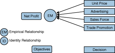
Figure 12.3 Empirical Relationships between Marketing Decisions and Objectives
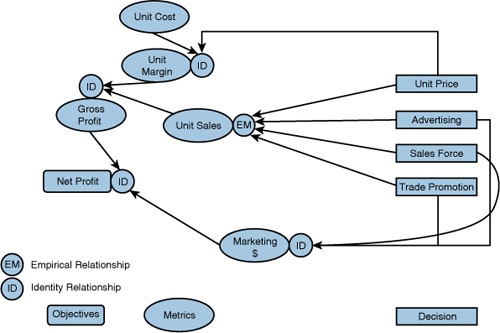
Figure 12.4 Empirical Relationship with Components of Marketing Outcomes
Marketing mix models are used to estimate the effects of marketing levers on marketing objectives and make decisions about how to allocate resources. One of the most frequently applied marketing mix models is the one underlying simulated test markets and depicted in Figure 12.5. With only minor variations, these models are used to forecast new product sales (see Section 4.1 for more detail). The structure of this model is straightforward, even if some would argue it is not simple. Forecast unit sales are calculated in a multiplicative identity from the metrics below. The multiplicative nature of the identity captures the most significant interactions of the marketing mix without resorting to (even more) complex equations. It is, we assert, more managerially transparent and useful because of this well-structured system of metrics that defines and separates identities from empirical relationships.
Forecast Unit Sales = Number of Consumer Prospects *Awareness * Availability *( Trial Rate * Trial Units + Repeat Rate * Repeat Units).
The input estimates for the components are obtained from the results of the simulated test, surveys, management judgment, and/or empirical models.
One of the advantages of the model in Figure 12.5 is that it also provides clear and separate paths by which the different marketing mix elements are believed to impact unit sales. Advertising affects Consumer Awareness but not Availability. Of course, in reality “everything affects everything,” but the KISS structure affords a transparency and utility that might be destroyed if management didn’t impose the discipline of focusing on the most important empirical relationships that the identity relationships suggest.
In the case of the new product forecasting model in Figure 12.5 we have decomposed (defined) the forecast sales to be a function of the metrics listed. The way we choose to decompose the objective may be more or less suitable for separating marketing mix empirical effects. For example, breaking down a share goal into share of requirements, heavy usage index, and penetration share would not have an obvious relationship to individual mix elements. Everything would still affect everything. So, not every identity will be helpful in a model of marketing mix effects.
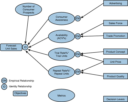
Figure 12.5 Simulated Test Markets Combine Empirical and Identity Relationships
Also, depending on how the data are collected, some identities may be strongly suggested by the data, even if they are not directly measured. For example, in consumer packaged goods markets, data on distribution (see Section 6.6) and channel promotion activity (incremental sales lift %—see Section 8.1) are regularly collected and reported to marketing managers. The availability of these two metrics strongly suggests the need for a third metric, “preference,” to create an attractive identity that may be useful in separating empirical effects and allowing for important interactions. Figure 12.6 shows how marketers might be able to “back into” values of preference by combining share, lift %, and distribution metrics. Of course, this approach means that the marketers are defining preference in a way that is consistent with relative choice under scenarios of equal distribution and lift %.
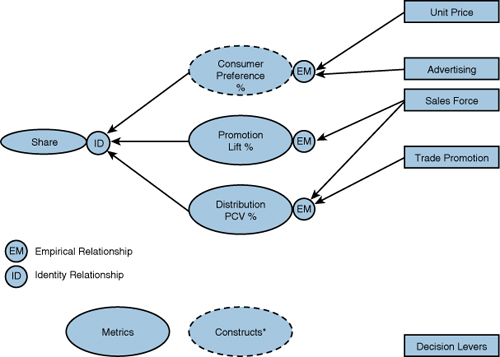
Figure 12.6 Empirical Relationship with Marketing Components and Intermediate Metrics and Constructs
Related Metrics and Concepts
By definition, accounting identities always hold. It is simply a matter of getting the correct values for the component parts. Other identities, such as those found in theoretical models of finance and economics, are true “in theory” or assuming certain conditions. For example, as discussed in Sections 7.3 and 7.4, at profit-maximizing levels of price, this identity should be true:
Margin on Sales [(Price – Variable Cost)/Price] = 1 price elasticity for constant elasticity demand, or
Price = Variable Cost + ½ (Maximum Willingness to Pay – Variable Cost) for linear demand functions
These identities identify relationships that are unlikely to be precise, but are vaguely right.
References and Suggested Further Reading
Hubbard, Douglas W. (2007). How to Measure Anything: Finding the Value of “Intangibles” in Business, John Wiley & Sons, Hoboken, New Jersey.
Appendix 1
Numerical Example
Consider a firm with estimated sales of $25,677 million last year. Although this is the number stated in the annual report, marketing managers know that this number is an estimate and not the actual sales. They judge the error in the estimate of sales to have a standard deviation of $3,000 million. This means they judge there to be about a 68% chance that actual sales is somewhere between $22,677 and $28,677 million. Keep in mind that if the managers wanted to assume that $25,677 million was, indeed, the actual sales figure, they would simply set the standard deviation of that estimate to zero.
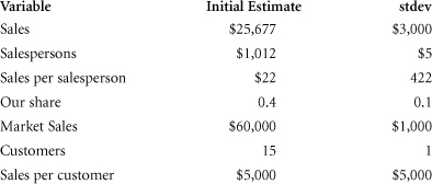
Similarly, the marketing managers came up with estimates and standard deviations for six outer-ring components of sales. In this particular example, we ignore vendor-related metrics. Note that both sales per salesperson and sales per customer have high standard deviations relative to their initial estimates. This reflects the fact that managers were not certain about these two metrics and would expect their initial estimates to be off by quite a bit.
Notice that we now have four ways to estimate sales: the initial estimate of $25,677 from the managers and three other pairs of initial estimates of components that can be combined (multiplied in this example) to also estimate sales. One way to proceed would be to calculate those three other estimates and average all four estimates to get our final estimate of sales. But we can do better than that. The unweighted average of the four estimates does not take advantage of the information we have on the quality of each of the initial estimates. Since sales per salesperson and sales per customer are very uncertain, we might want to pay more attention to (give more weight to) the estimate we get using the share and total sales estimates.
The process we propose for combining the initial estimates (and their quality measures) into one set of final estimates is logical and straightforward. First, we want to find a set of final estimates that satisfy the three identities (our final estimate of sales should equal our final estimate of salespersons times our final estimate of sales per salesperson, for example). And from among the many sets of final estimates that satisfy all the identities, we want to find the one that is “closest” to the managers’ initial estimates—where closeness is measured in units of standard deviation.
In summary, our final estimates will be the set of metrics “closest” to our initial estimates that satisfy all the identities in our model. Our final estimates will be internally consistent and as close as possible to the initial set of estimates (which were not internally consistent).
Conclusion
“… metrics should be necessary (i.e., the company cannot do without them), precise, consistent, and sufficient (i.e., comprehensive) for review purposes.”4
Understanding metrics will allow marketers to choose the right input data to give them meaningful information. They should be able to pick and choose from a variety of metrics depending upon the circumstances and create a dashboard of the most vital metrics to aid them in managing their business. After reading this work, we hope you agree that no one metric is going to give a full picture. It is only when you can use multiple viewpoints that you are likely to obtain anything approaching a full picture.
“… results measures tell us where we stand in efforts to achieve goals, but not how we go there or what to do differently”.5
Marketing metrics are needed to give a complete picture of a business’s health. Financial metrics focus on dollars and periods of time, telling us how profits, cash, and assets are changing. However, we also need to understand what is happening with our customers, products, prices, channels, competitors, and brands.
The interpretation of marketing metrics requires knowledge and judgment. This book helps give you the knowledge so that you can know more about how metrics are constructed and what they measure. Knowing the limitations of individual metrics is important. In our experience, businesses are usually complex, requiring multiple metrics to capture different facets—to tell you what is going on.
Because of this complexity, marketing metrics often raise as many questions as they answer. Certainly, they rarely provide easy answers about what managers should do. Having a set of metrics based on a limited, faulty, or outmoded view of the business can also blind you. Such a set of metrics can falsely reassure you that the business is fine when in fact trouble is developing. Like the ostrich with his head in the sand, it might be more comfortable to know less.
We don’t expect that a command of marketing metrics will make your job easier. We do expect that such knowledge will help you do your job better.