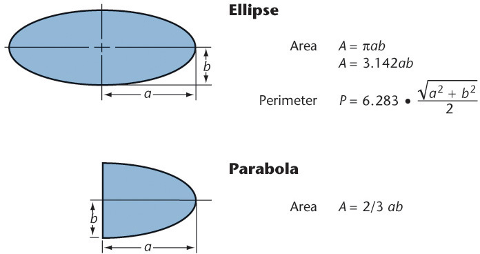
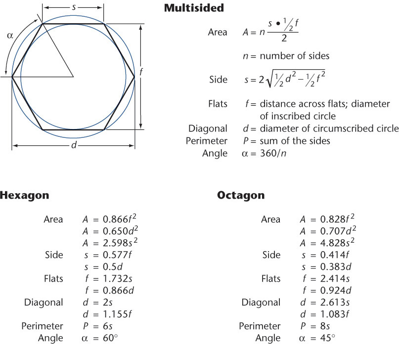
Formulas for Regular Polygons
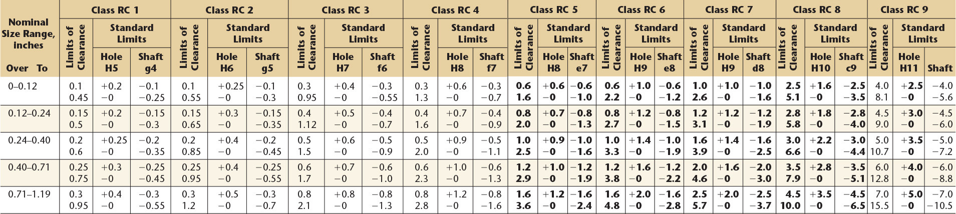
4 Running and Sliding Fitsa—American National Standard
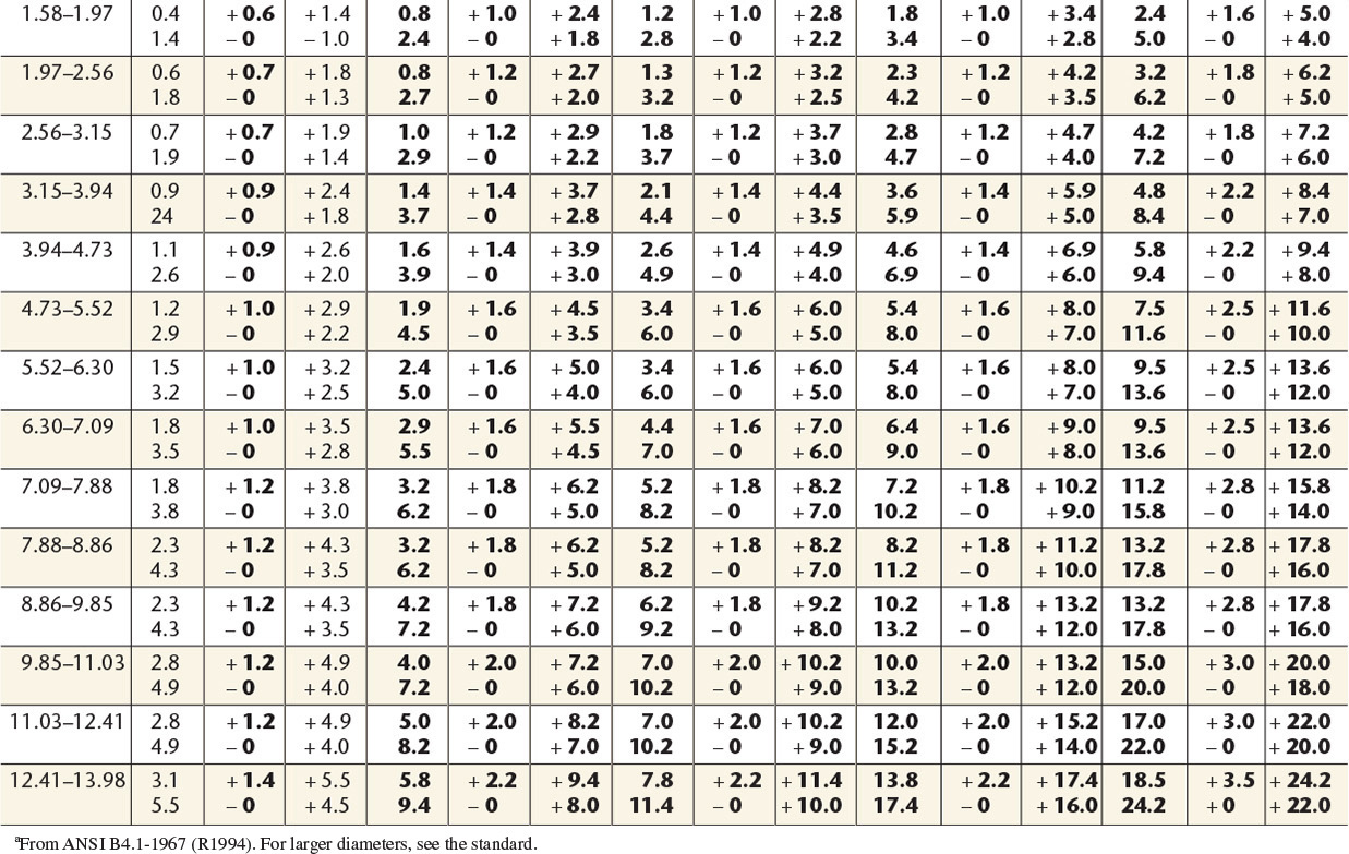
aFrom ANSI B4.1-1967 (Rl994). For larger diameters, see the standard.
RC 1
Close sliding fits are intended for the accurate location of parts which must assemble without perceptible play.
RC 2
Sliding fits are intended for accurate location, but with greater maximum clearance than class RC 1. Parts made to this fit move and turn easily but are not intended to run freely, and in the larger sizes may seize with small temperature changes.
RC 3
Precision running fits are about the closest fits which can be expected to run freely and are intended for precision work at slow speeds and light journal pressures, but they are not suitable where appreciable temperature differences are likely to be encountered.
RC 4
Close running fits are intended chiefly for running fits on accurate machinery with moderate surface speeds and journal pressures, where accurate location and minimum play are desired.
Basic hole system. Limits are in thousandths of an inch. Limits for hole and shaft are applied algebraically to the basic size to obtain the limits of size for the parts. Data in boldface are in accordance with ABC agreements. Symbols H5, g5, etc., are hole and shaft designations used in ABC System.

![]()
Medium running fits are intended for higher running speeds, or heavy journal pressures, or both.
RC 7
Free running fits are intended for use where accuracy is not essential, or where large temperature variations are likely to be encountered, or under both these conditions.
![]()
Loose running fits are intended for use where wide commercial tolerances may be necessary, together with an allowance, on the external member.
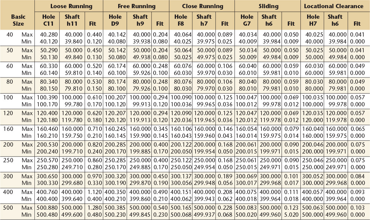
5 Clearance Locational Fitsa—American National Standard
aFrom ANSI B4.1-1967 (R1994). For larger diameters, see the standard.
LC
Locational clearance fits are intended for parts which are normally stationary but which can be freely assembled or disassembled. They run from snug fits for parts requiring accuracy of location, through the medium clearance fits for parts such as spigots, to the looser fastener fits, where freedom of assembly is of prime importance.
Basic hole system. Limits are in thousandths of an inch. Limits for hole and shaft are applied algebraically to the basic size to obtain the limits of size for the parts. Data in boldface are in accordance with ABC agreements. Symbols H6, H5, etc., are hole and shaft designations used in ABC System.


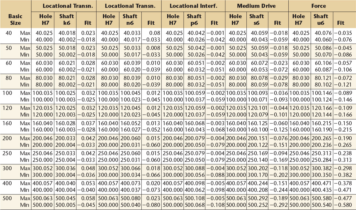
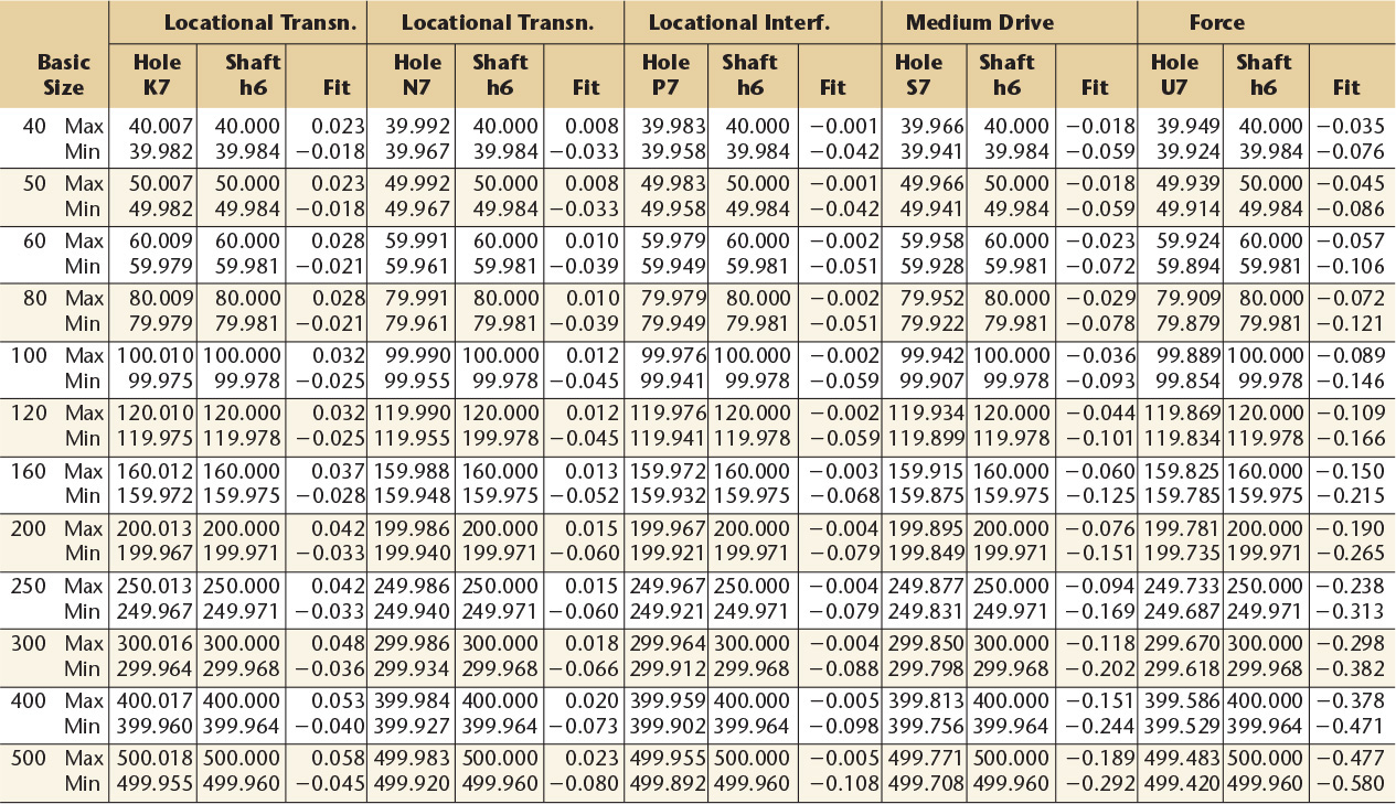
6 Transition Locational Fitsa—American National Standard
aFrom ANSI B4.1-1967 (R1994). For larger diameters, see the standard.
LT
Transition fits are a compromise between clearance and interference fits, for application where accuracy of location is important, but either a small amount of clearance or interference is permissible.
Basic hole system. Limits are in thousandths of an inch. Limits for hole and shaft are applied algebraically to the basic size to obtain the limits of size for the mating parts. Data in boldface are in accordance with ABC agreements. “Fit” represents the maximum interference (minus values) and the maximum clearance (plus values). Symbols H7, js6, etc., are hole and shaft designations used in ABC System.

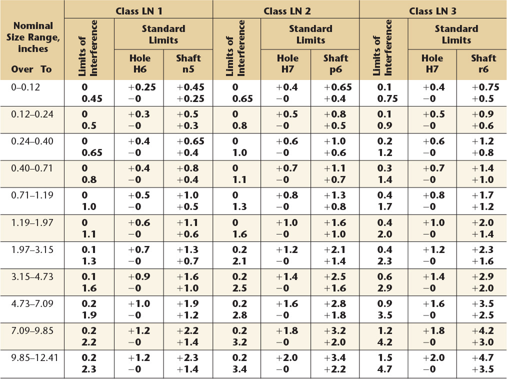
7 Interference Locational Fitsa—American National Standard
aFrom ANSI B4.1-1967 (R1994). For larger diameters, see the standard.
LN
Locational interference fits are used where accuracy of location is of prime importance and for parts requiring rigidity and alignment with no special requirements for bore pressure. Such fits are not intended for parts designed to transmit frictional loads from one part to another by virtue of the tightness of fit, as these conditions are covered by force fits.
Basic hole system. Limits are in thousandths of an inch. Limits for hole and shaft are applied algebraically to the basic size to obtain the limits of size for the parts. Data in boldface are in accordance with ABC agreements. Symbols H7, p6, etc., are hole and shaft designations used in ABC System.
Light drive fits are those requiring light assembly pressures, and produce more or less permanent assemblies. They are suitable for thin sections or long fits, or in cast-iron external members.
FN 2
Medium drive fits are suitable for ordinary steel parts, or for shrink fits on light sections. They are about the tightest fits that can be used with high-grade cast-iron external members.
FN 3
Heavy drive fits are suitable for heavier steel parts or for shrink fits in medium sections.
![]()
Force fits are suitable for parts which can be highly stressed, or for shrink fits where the heavy pressing forces required are impractical.
Basic hole system. Limits are in thousandths of an inch. Limits for hole and shaft are applied algebraically to the basic size to obtain the limits of size for the parts. Data in boldface are in accordance with ABC agreements. Symbols H7, s6, etc., are hole and shaft designations used in ABC System.


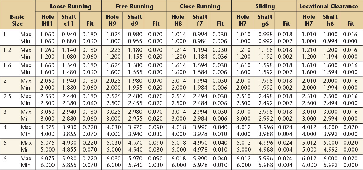
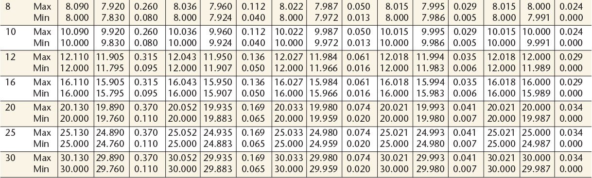
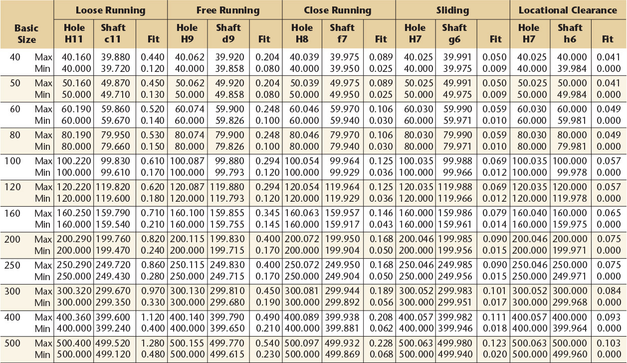
10 Preferred Metric Hole Basis Clearance Fitsa—American National Standard
aFrom ANSI B4.2-1978 (R1994).
Dimensions are in millimeters.
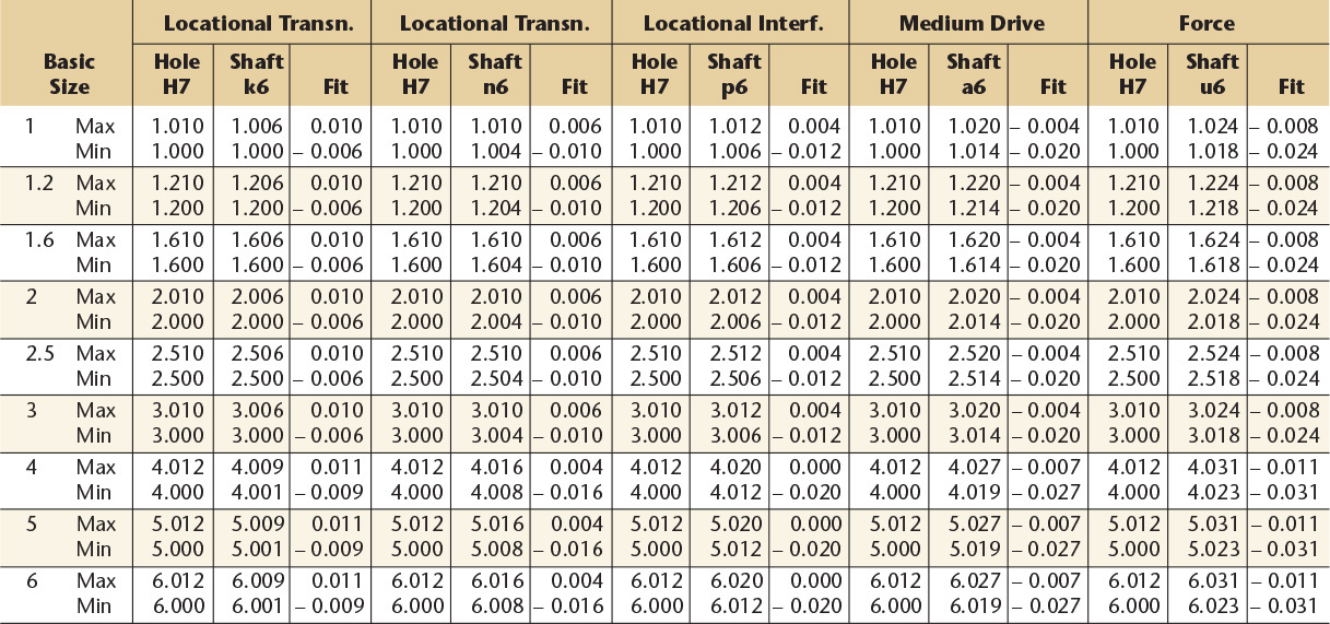
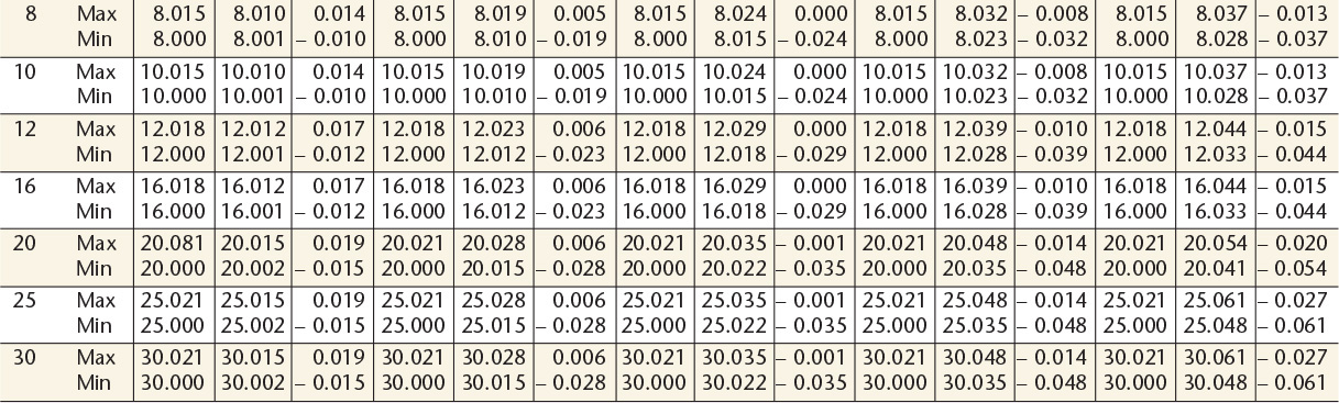
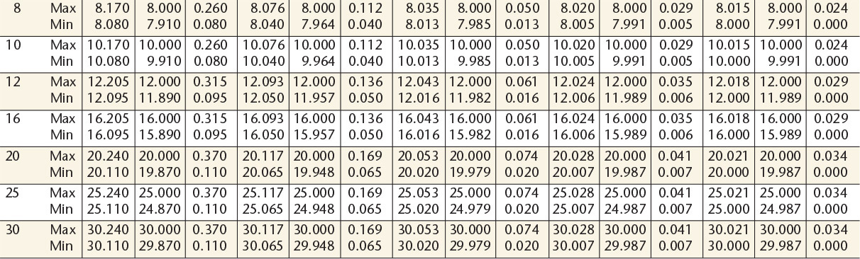
11 Preferred Metric Hole Basis Transition and Interference Fitsa—American National Standard
aFrom ANSl B4.2-1978 (R1994).
Dimensions are in millimeters.
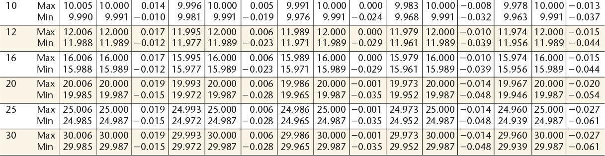
12 Preferred Metric Shaft Basis Clearance Fitsa—American National Standard
aFrom ANSI B4.2-1978 (R1994).
Dimensions are in millimeters.

13 Preferred Metric Shaft Basis Transition and Interference Fitsa—American National Standard
aFrom ANSI B4.2-1978 (R1994).
Dimensions are in millimeters.

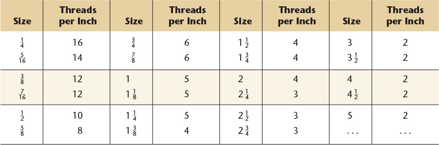
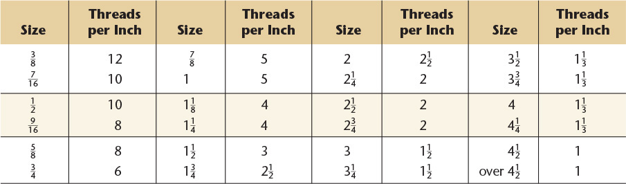
14 Screw Threads, American National, Unified, and Metric
American National Standard Unified and American National Screw Threads.a
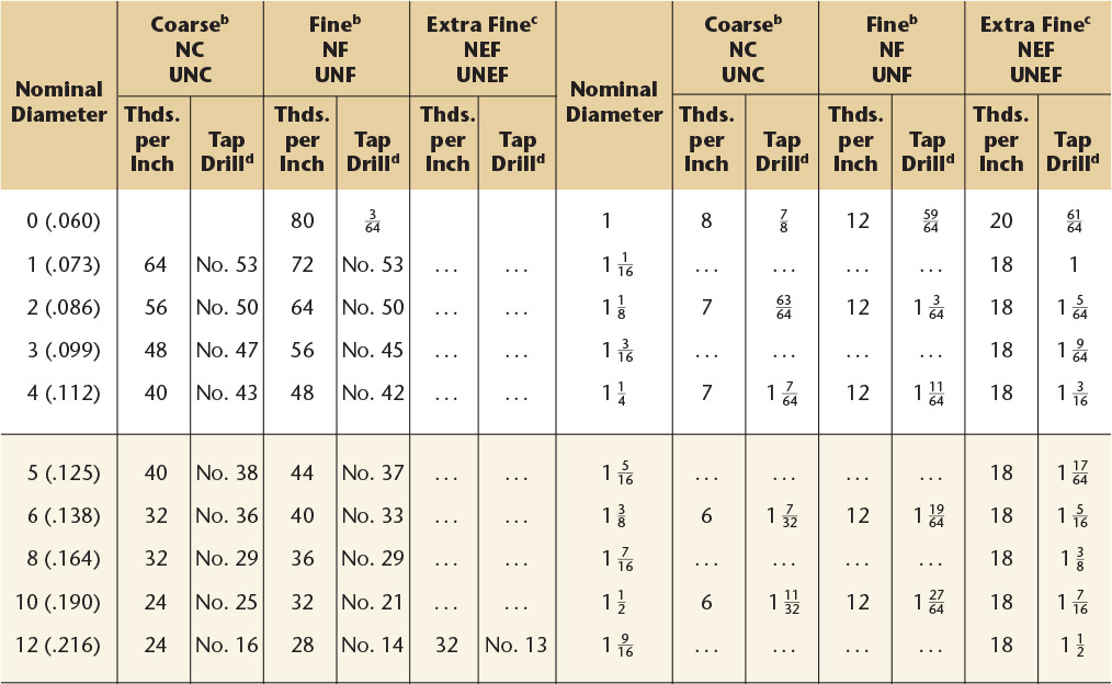
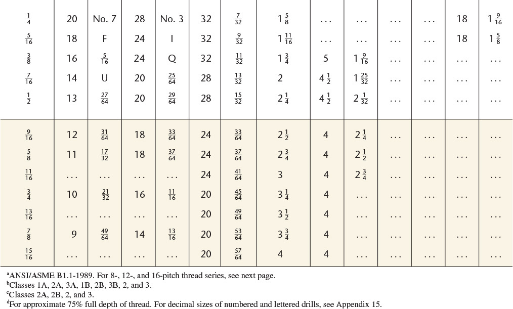
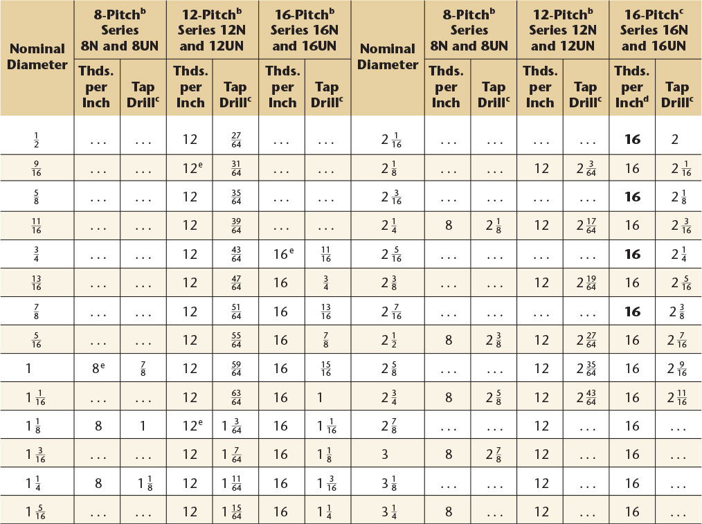
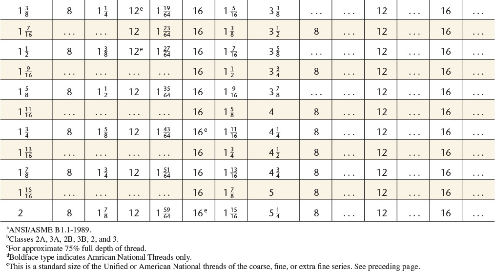
Preferred sizes for commercial threads and fasteners are shown in boldface type.
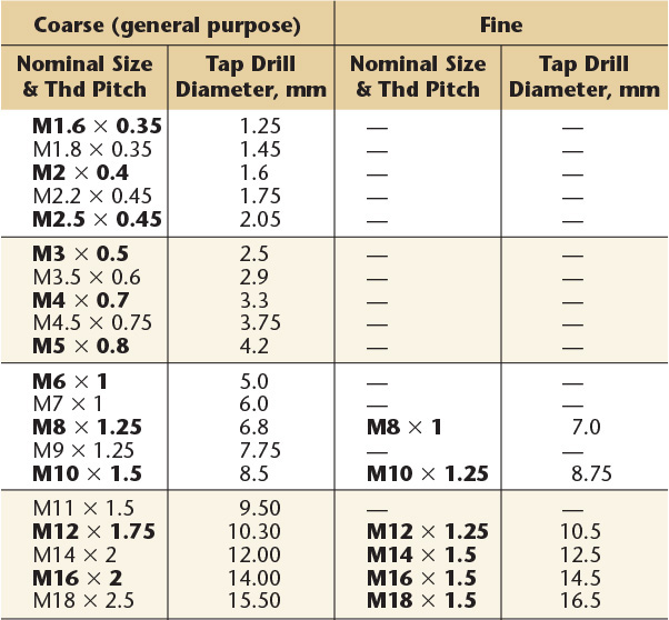

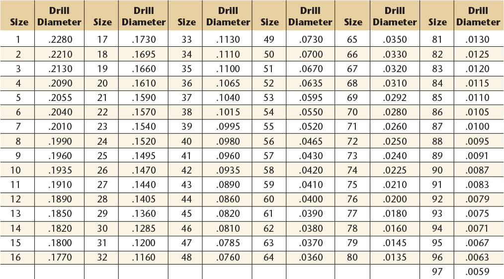
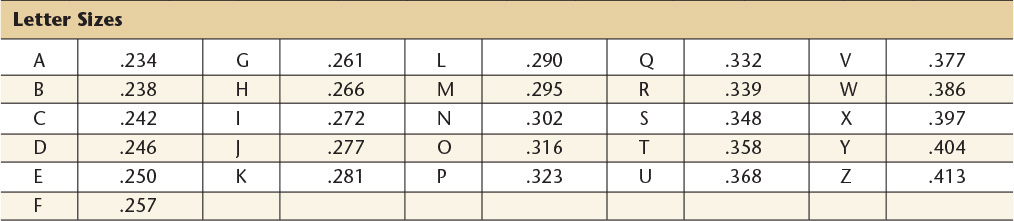
15 Twist Drill Sizes—American National Standard and Metric
American National Standard Drill Sizes.a All dimensions are in inches. Drills designated in common fractions are available in diameters ![]() ″ to
″ to ![]() ″ in
″ in ![]() ″ increments,
″ increments, ![]() ″ to
″ to ![]() ″ in
″ in ![]() ″ increments.
″ increments. ![]() ″ to 3″ in
″ to 3″ in ![]() ″ increments and 3″ to
″ increments and 3″ to ![]() ″ in
″ in ![]() ″ increments. Drills larger than
″ increments. Drills larger than ![]() ″ are seldom used, and are regarded as special drills.
″ are seldom used, and are regarded as special drills.
aANSI/ASME B94.11M-1993.
Metric Drill Sizes. Decimal inch equivalents are for reference only.


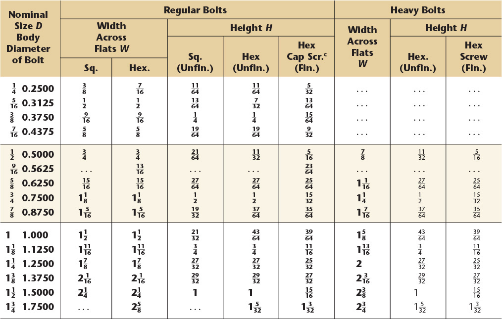
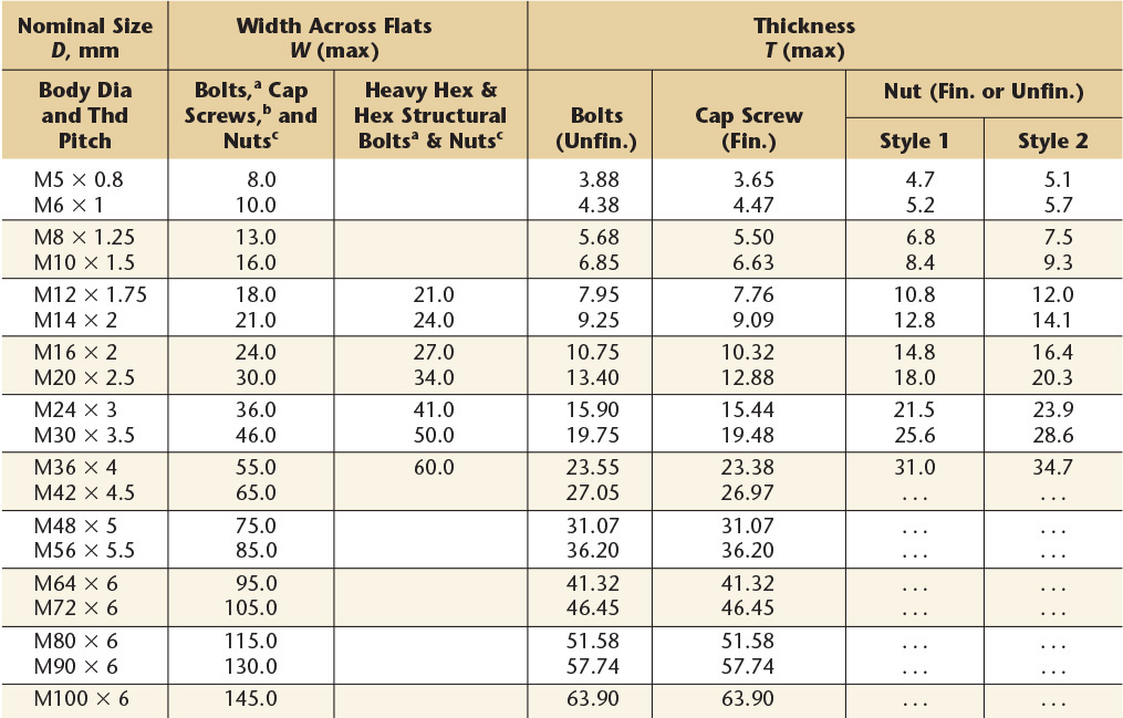
17 Bolts, Nuts, and Cap Screws—Square and Hexagon—American National Standard and Metric
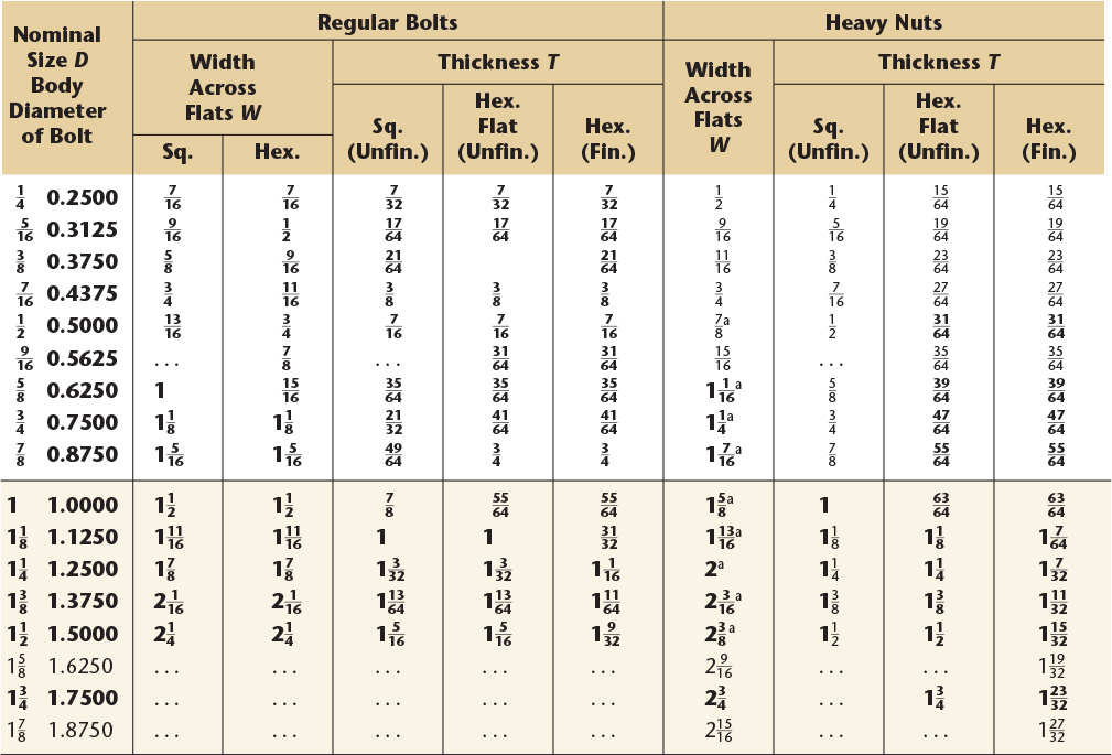
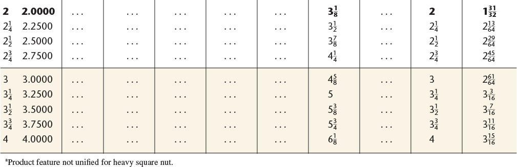
American National Standard Square and Hexagon Boltsa and Nutsb and Hexagon Cap Screws.c Boldface type indicates product features unified dimensionally with British and Canadian standards. All dimensions are in inches.
aANSI B18.2.1-1981 (R1992).
bANSI/ASME B18.2.2.-1987 (R1993).
cHexagon cap screws and finished hexagon bolts are combined as a single product.

American National Standard Square and Hexagon Bolts and Nuts and Hexagon Cap Screws (continued). See ANSI B18.2.2 for jam nuts, slotted nuts, thick nuts, thick slotted nuts, and castle nuts.
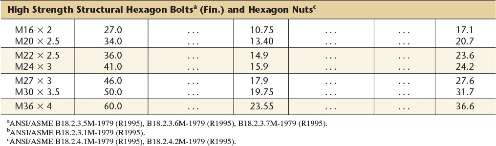
Metric hexagon bolts, hexagon cap screws, hexagon structural bolts, and hexagon nuts.
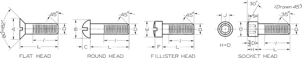
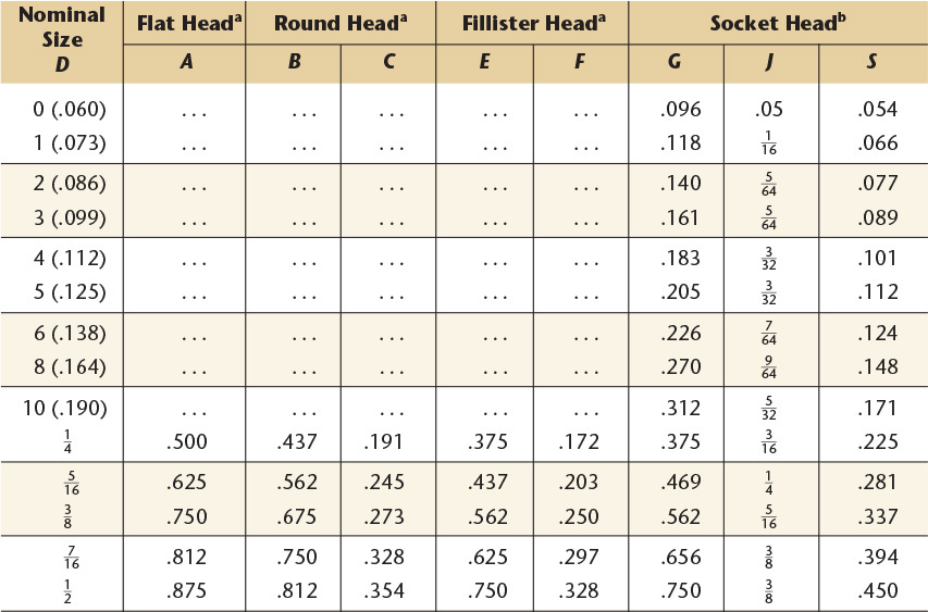
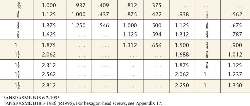

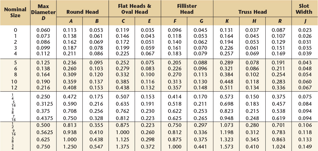
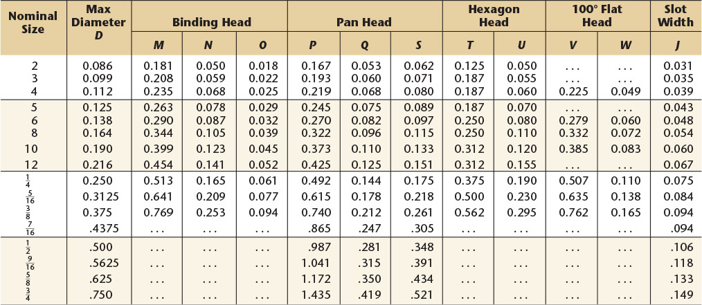
American National Standard machine screws.
Length of Thread: On screws 2″ long and shorter, the threads extend to within two threads of the head and closer if practical; longer screws have minimum thread length of ![]() ″.
″.
Points: Machine screws are regularly made with plain sheared ends, not chamfered.
Threads: Either Coarse or Fine Thread Series, Class 2 fit.
Recessed Heads: Two styles of cross recesses are available on all screws except hexagon head.
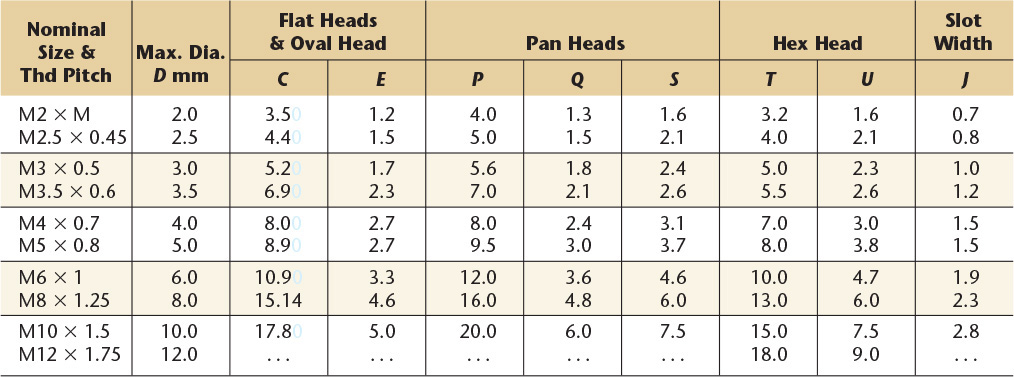
Length of Thread: On screws 36 mm long or shorter, the threads extend to within one thread of the head: on longer screws the thread extends to within two threads of the head.
Points: Machine screws are regularly made with sheared ends, not chamfered.
Threads: Coarse (general purpose) threads series are given.
Recessed Heads: Two styles of cross-recesses are available on all screws except hexagon head.
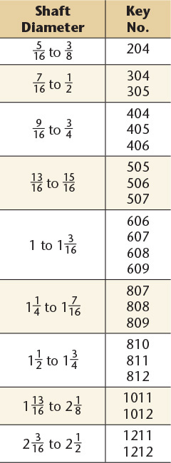
20 Keys—Square, Flat, Plain Taper,a and Gib Head
a Plain taper square and at keys have the same dimensions as the plain parallel stock keys, with the addition of the taper on top. Gib head taper square and at keys have the same dimensions as the plain taper keys, with the addition of the gib head. Stock lengths for plain taper and gib head taper keys: The minimum stock length equals 4W, and the maximum equals 16W. The increments of increase of length equal 2W.
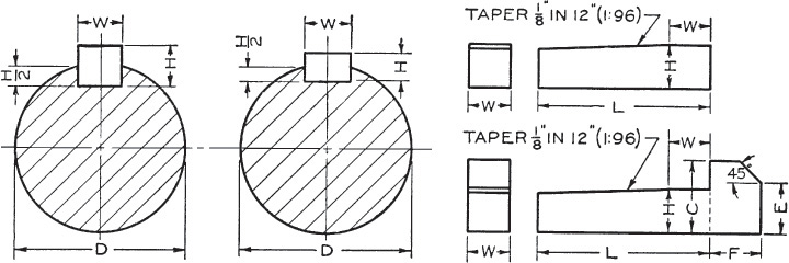


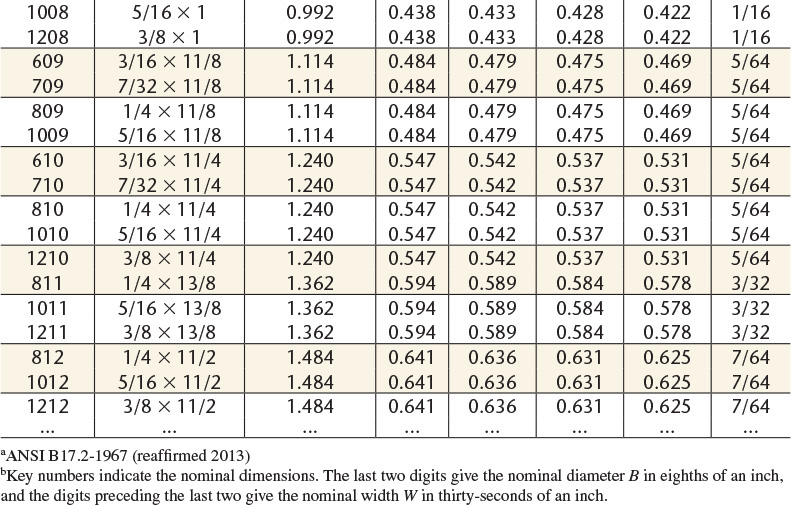

Maximum length of slot is 4”+ W. Note that key is sunk two-thirds into shaft in all cases.


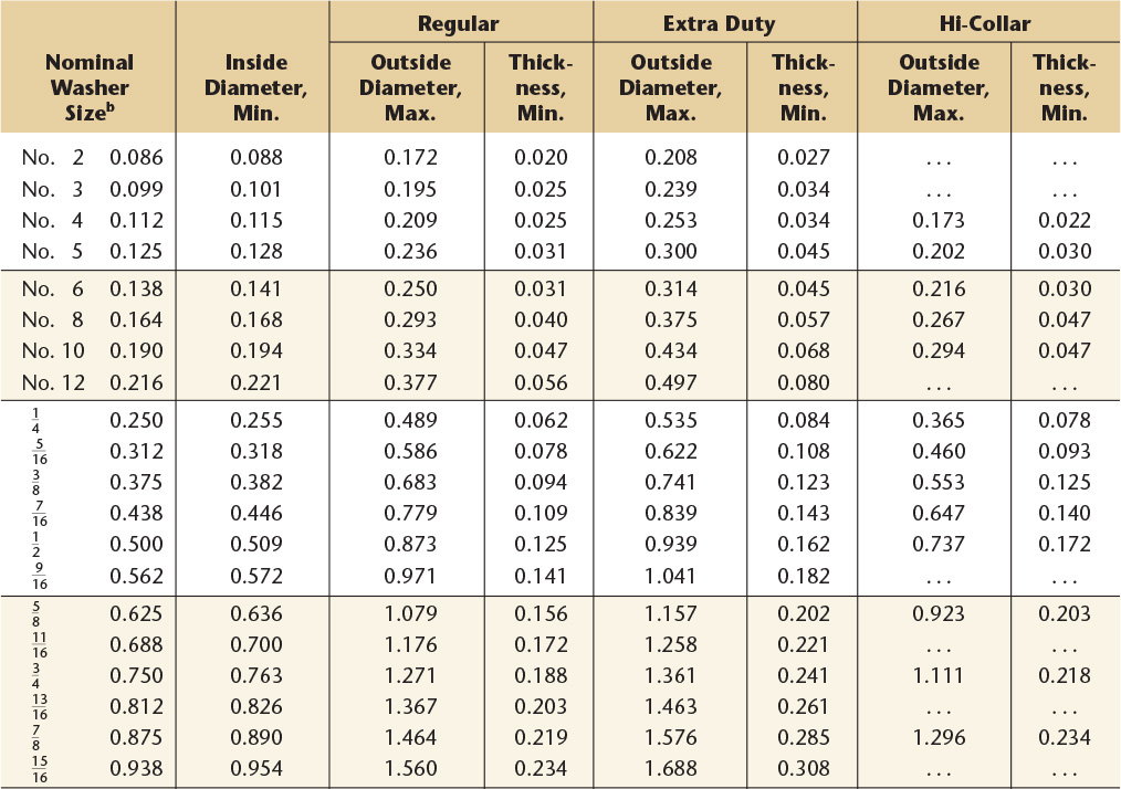
For parts lists, etc., give inside diameter, outside diameter, and the thickness; for example, .344 × .688 × .065 Type A Plain Washer. Preferred Sizes of Type A Plain Washers.b


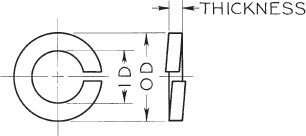
For parts lists, etc., give nominal size and series; for example, ![]() regular lock washer (preferred series).
regular lock washer (preferred series).


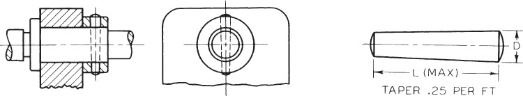
To find small diameter of pin, multiply the length by .02083 and subtract the result from the larger diameter. All dimensions are given in inches. Standard reamers are available for pins given above the heavy line.
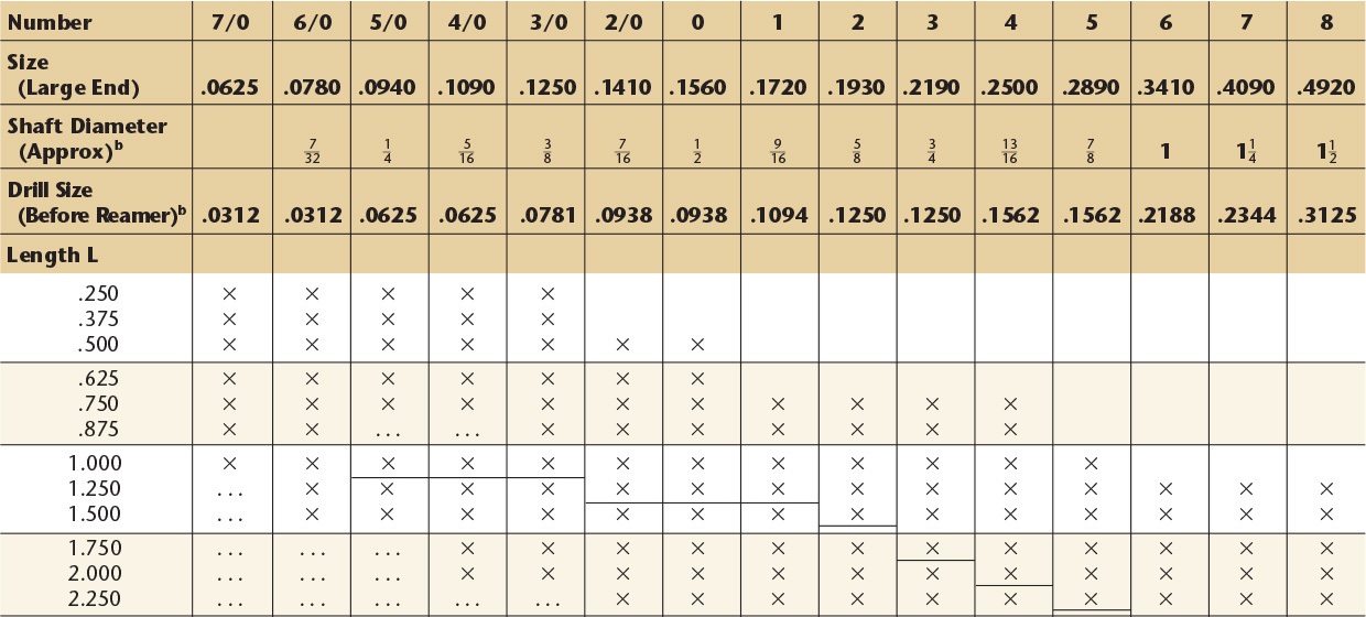

All dimensions are given in inches.


34 Heating, Ventilating, and Ductwork Symbolsa—American National Standard
a ANSI/ASME Y32.2.3-1949 (R1994) and ANSI Y32.2.4-1949 (R1993).

36 Form and Proportion of Datum Symbolsa
aReprinted from ASME Y14.5-2009, by permission of The American Society of Mechanical Engineers. All rights reserved.

37 Form and Proportion of Geometric Characteristic Symbolsa
aReprinted from ASME Y14.5-2009, by permission of The American Society of Mechanical Engineers. All rights reserved.

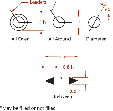
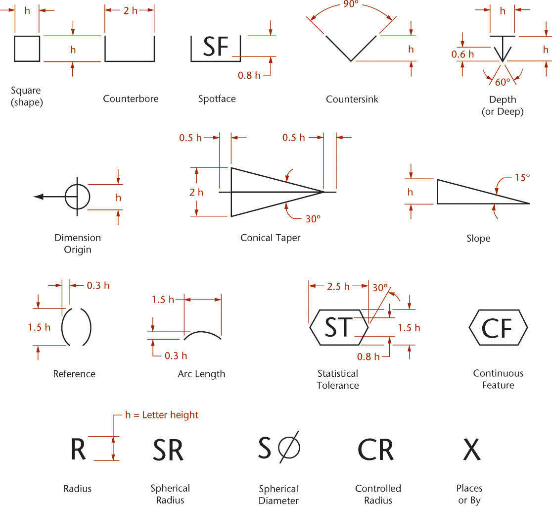
38 Form and Proportion of Geometric Dimensioning Symbolsa
aReprinted from ASME Y14.5M-2009, by permission of The American Society of Mechanical Engineers. All rights reserved.
39 Form and Proportion of Modifying Symbolsa
aReprinted from ASME Y14.5M-2009, by permission of The American Society of Mechanical Engineers. All rights reserved.

40 Form and Proportion of Dimensioning Symbols and Lettersa
aReprinted from ASME Y14.5M-2009, by permission of The American Society of Mechanical Engineers. All rights reserved.
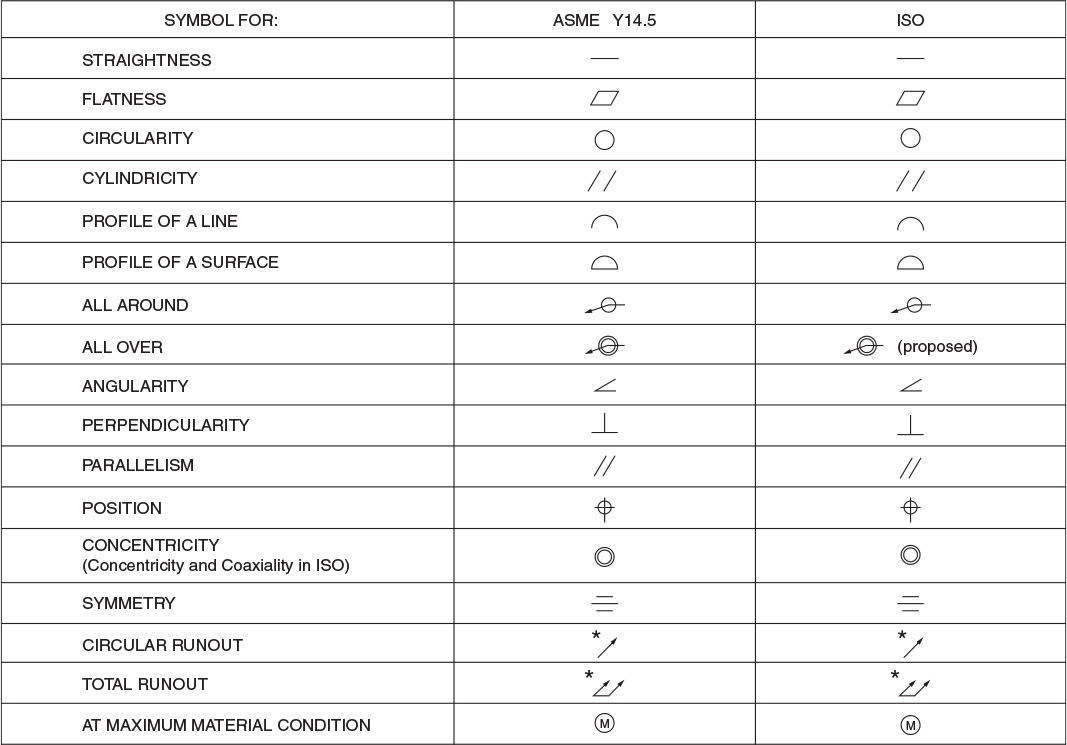
41 Comparison of Symbolsa
aReprinted from ASME Y14.5-2009, by permission of The American Society of Mechanical Engineers. All rights reserved.

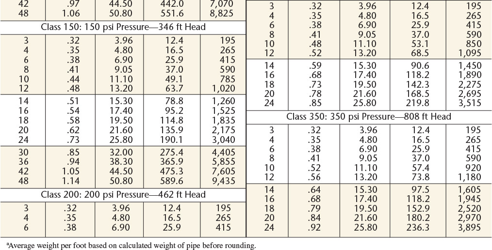
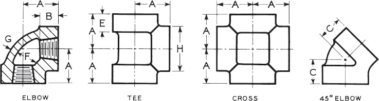
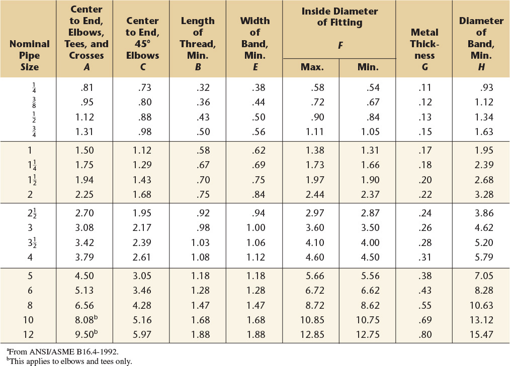
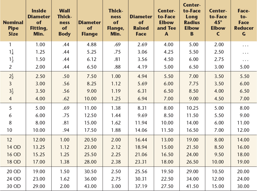
Dimensions of 90° and 45° elbows, tees, and crosses (straight sizes). All dimensions given in inches. Fittings having right- and left-hand threads shall have four or more ribs or the letter “L” cast on the band at end with left-hand thread.

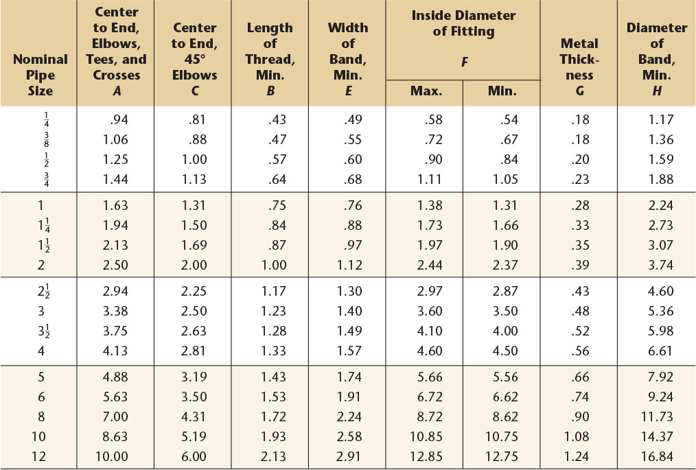
Dimensions of 90° and 45° elbows, tees, and crosses (straight sizes). All dimensions given in inches. The 250-lb standard for screwed fittings covers only the straight sizes of 90° and 45° elbows, tees, and crosses.
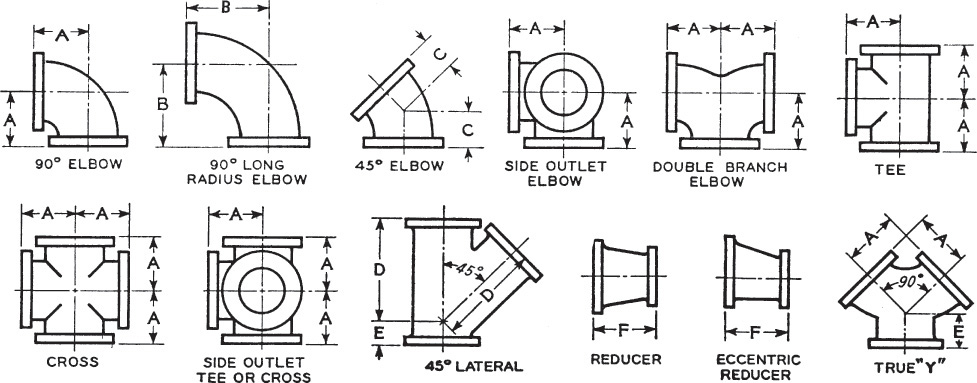
Dimensions of elbows, double branch elbows, tees, crosses, laterals, true Y’s (straight sizes), and reducers. All dimensions in inches.


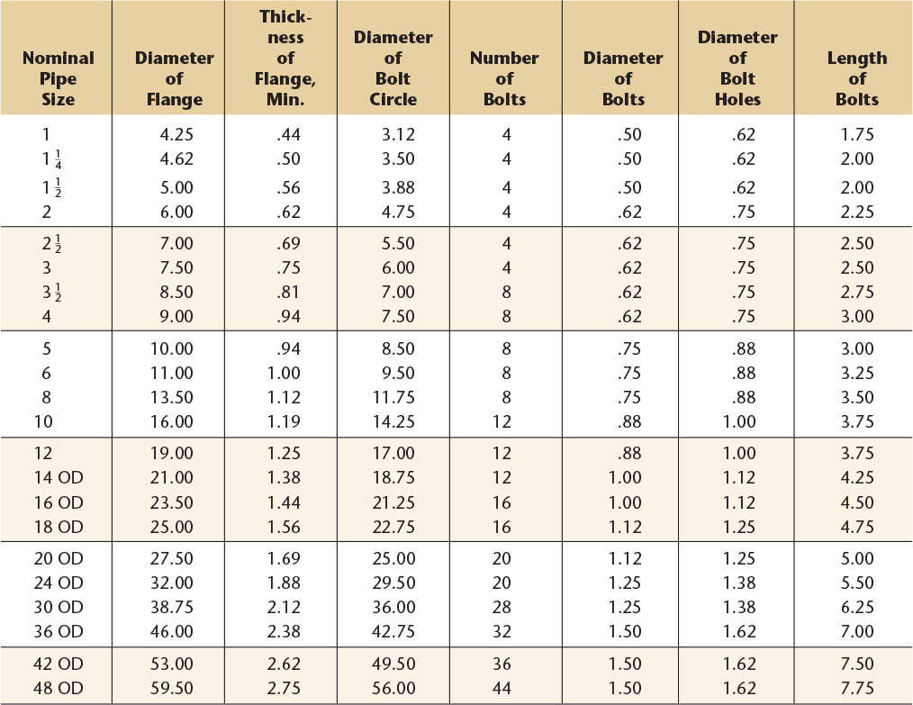
47 Cast Iron Pipe Flanges, Drilling for Bolts and Their Lengths,a 125 lb—American National Standard
a ANSI B16.1-1989.
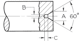
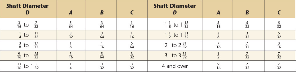
48 Shaft Center Sizes
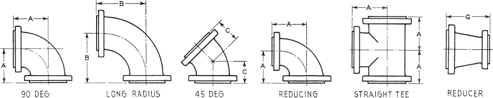
Dimensions of elbows, tees, and reducers. All dimensions are given in inches.
50 Cast Iron Pipe Flanges, Drilling for Bolts and Their Lengths,a 250 lb—American National Standard
a ANSI B16.1-1989.

51 Types of Scales
Scales are measuring tools used to quickly enlarge or reduce drawing measurements. Figure A51.1 shows a number of scales, including (a) metric, (b) engineers’, (c) decimal, (d) mechanical engineers’, and (e) architects’ scales. On a full-divided scale, the basic units are subdivided throughout the length of the scale. On open-divided scales, such as the architects’ scale, only the end unit is subdivided.

Scales are usually made of plastic or boxwood. The better wood scales have white plastic edges. Scales can be either triangular or flat. The triangular scales combine several scales on one stick by using each of the triangle’s three sides. A scale guard, shown in Figure A51.1f, can save time and prevent errors by indicating the side of the scale currently in use.
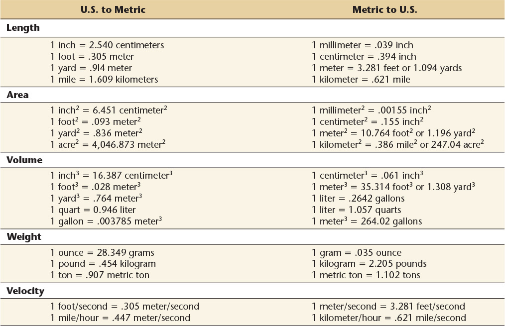
Several scales that are based on the inch-foot system of measurement continue in domestic use today, along with the metric system of measurement, which is accepted worldwide for science, technology, and international trade.
Metric Scales
Metric scales are available in flat and triangular styles with a variety of scale graduations. The triangular scale illustrated (Figure A51.2) has one full-size scale and five reduced-size scales, all fully divided. With these scales, a drawing can be made full size, enlarged sized, or reduced sized.

Full Size
The 1:1 scale (Figure A51.2a, top) is full size, and each division is actually 1 mm in width with the calibrations numbered at 10-mm intervals. The same scale is also convenient for ratios of 1:10, 1:100, 1:1000, and so on.
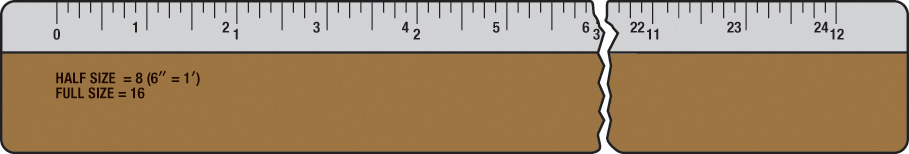
Half Size
The 1:2 scale (Figure A51.2a, bottom) is half size, and each division equals 2 mm with the calibration numbering at 20-unit intervals. This scale is also convenient for ratios of 1:20, 1:200, 1:2000, and so on.
The remaining four scales on this triangular metric scale include the typical scale ratios of 1:5, 1:25, and 1:75 (Figures A51.2b and c). These ratios may also be enlarged or reduced by multiplying or dividing by a factor of 10. Metric scales are also available with other scale ratios for specific drawing purposes.
Metric scales are also used in map drawing and in drawing force diagrams or other graphical constructions that involve such scales as 1 mm = 1 kg and 1 mm = 500 kg.
Engineers’ Scales
An engineers’ scale is a decimal scale graduated in units of 1 inch divided into 10, 20, 30, 40, 50, and 60 parts. These scales are also frequently called civil engineers’ scales because they were originally used in civil engineering to draw large-scale structures or maps. Sometimes the engineers’ scale is referred to as a chain scale, because it derived from a chain of 100 links that surveyors used for land measurements.
Because the engineers’ scale divides inches into decimal units, it is convenient in machine drawing to set off inch dimensions expressed in decimals. For example, to set off 1.650″ full size, use the 10 scale and simply set off one main division plus 6-1/2 subdivisions (Figure A51.3). To set off the same dimension half size, use the 20 scale, since the 20 scale is exactly half the size of the 10 scale. Similarly, to set off the dimension quarter size, use the 40 scale.

An engineers’ scale is also used in drawing stress diagrams or other graphical constructions to such scales as 1″ = 20 lb and 1″ = 4000 lb.
Decimal-Inch Scales
The widespread use of decimal-inch dimensions brought about a scale specifically for that use. On its full-size scale, each inch is divided into fiftieths of an inch, or .02″. On half- and quarter-size decimal scales, the inches are compressed to half size or quarter size and then are divided into 10 parts, so that each subdivision stands for .1″ (Figure A51.4).

Mechanical Engineers’ Scales
The objects represented in machine drawing vary in size from small parts that measure only fractions of an inch to parts of large dimensions. For this reason, mechanical engineers’ scales are divided into units representing inches to full size, half size, quarter size, or eighth size (Figure A51.5). To draw an object to a scale of half size, for example, use the mechanical engineers’ scale marked half size, which is graduated so that every 1/2″ represents 1″. In other words, the half-size scale is simply a full-size scale compressed to half size.
These scales are useful in dividing dimensions. For example, to draw a 3.6″-diameter circle full size, it is necessary to use half of 3.6″ as the radius. Instead of using math to find half of 3.6″, it is easier to set off 3.6″ on the half-size scale.
Tip
Triangular combination scales are available that include full- and half-size mechanical engineers’ scales, several architects’ scales, and an engineers’ scale all on one stick.
52 Additional Geometric Constructions
Drawing an Approximate Ellipse
For many purposes, particularly where a small ellipse is required, use the approximate circular arc method (Figure A52.1). Such an ellipse is sure to be symmetrical and is quick to draw.
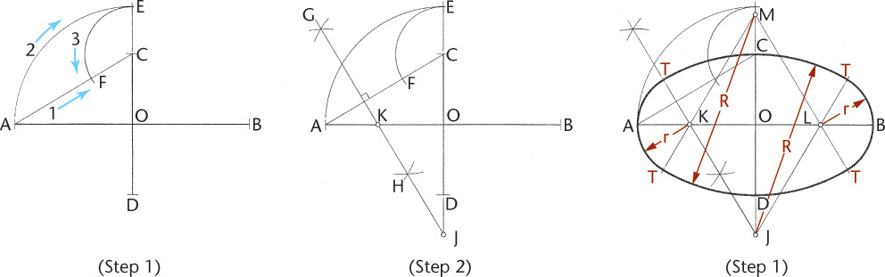
Given axes AB and CD,
Step 1. Draw line AC. With O as center and OA as radius, draw the arc AE. With C as center and CE as radius, draw the arc EF.
Step 2. Draw perpendicular bisector GH of the line AF; the points K and J, where they intersect the axes, are centers of the required arcs.
Step 3. Find centers M and L by setting off OL = OK and OM = OJ. Using centers K, L, M, and J, draw circular arcs as shown. The points of tangency T are at the junctures of the arcs on the lines joining the centers.
Tip
An ordinary piece of solder wire can be used very successfully by bending the wire to the desired curve.
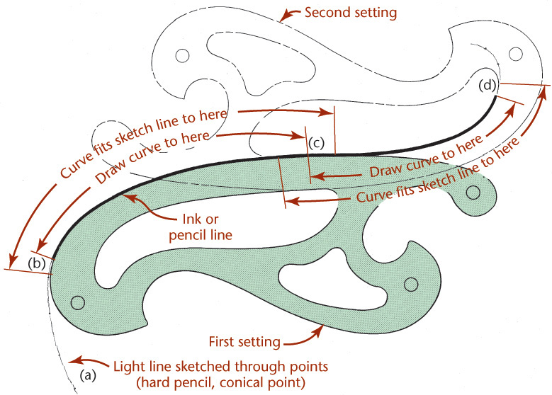
First, lightly sketch a curve through the points you have determined. Then, match the irregular curve along your lightly sketched pencil line for some distance beyond the segment to be drawn. This aids in creating curve portions that blend smoothly together at their tangencies. Try to avoid drawing below the curve.
Drawing a Parabola
The curve of intersection between a right circular cone and a plane parallel to one of its elements is a parabola (see Figure A52.2d). The parabola is used to reflect surfaces for light and sound, for vertical curves in highways, for forms of arches, and approximately for forms of the curves of cables for suspension bridges. It is also used to show the bending moment at any point on a uniformly loaded beam or girder.

A parabola is generated by a point moving so that its distances from a fixed point, the focus, and from a fixed line, the directrix, remain equal.
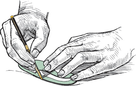
Focus F and directrix AB are given. A parabola may be generated by a pencil guided by a string (Figure A52.3a). Fasten the string at F and C; its length is GC. The point C is selected at random; its distance from G depends on the desired extent of the curve. Keep the string taut and the pencil against the T-square, as shown.

Given focus F and directrix AB, draw a line DE parallel to the directrix and at any distance CZ from it (Figure A52.3b). With center at F and radius CZ, draw arcs to intersect line DE at the points Q and R, which are points on the parabola. Determine as many additional points as are necessary to draw the parabola accurately, by drawing additional lines parallel to line AB and proceeding in the same manner.
A tangent to the parabola at any point G bisects the angle formed by the focal line FG and the line SG perpendicular to the directrix.
Given the rise and span of the parabola (Figure A52.3c), divide AO into any number of equal parts, and divide AD into a number of equal parts amounting to the square of that number. From line AB, each point on the parabola is offset by a number of units equal to the square of the number of units from point O. For example, point 3 projects 9 units (the square of 3). This method is generally used for drawing parabolic arches.
To find the focus, F, given points P, R, and V of a parabola (Figure A52.3d), draw a tangent at P, making a = b. Draw the perpendicular bisector of AP, which intersects the axis at F, the focus of the parabola.
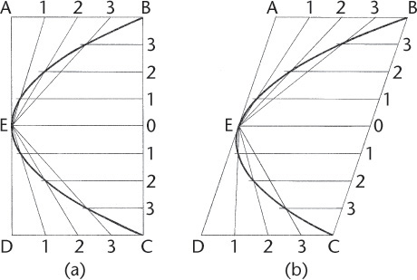
Draw a parabola given rectangle or parallelogram ABCD (Figure A52.4a and b). Divide BC into any even number of equal parts, divide the sides AB and DC each into half as many parts, and draw lines as shown. The intersections of like-numbered lines are points on the parabola.
Joining Two Points by a Parabolic Curve
Let X and Y be the given points (Figure A52.5). Assume any point O, and draw tangents XO and YO. Divide XO and YO into the same number of equal parts, number the division points as shown, and connect corresponding points. These lines are tangents of the required parabola and form its envelope. Sketch a light smooth curve, and then darken the curve with the aid of an irregular curve.

These parabolic curves are more pleasing in appearance than circular arcs and are useful in machine design. If the tangents OX and OY are equal, the axis of the parabola will bisect the angle between them.
Tip: Irregular Curves
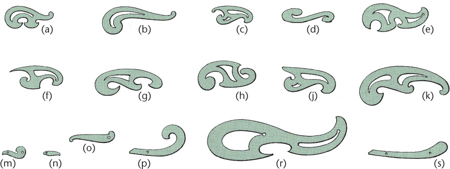
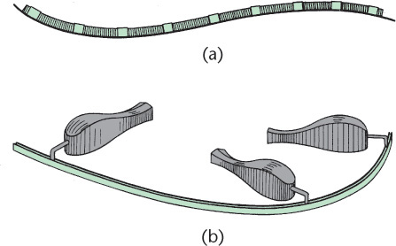
The curves are largely successive segments of geometric curves, such as the ellipse, parabola, hyperbola, and involute. Among the many special types of curves available are hyperbolas, parabolas, ellipses, logarithmic spirals, ship curves, and railroad curves. Adjustable curves consist of a core of lead, enclosed by a coil spring attached to a flexible strip. The figure shows a spline to which “ducks” (weights) are attached. The spline can be bent to form any desired curve, limited by the elasticity of the material.
Drawing a Hyperbola
The curve of intersection between a right circular cone and a plane making an angle with the axis smaller than that made by the elements is a hyperbola (see Figure A52.2e). A hyperbola is generated by a point moving so that the difference of its distances from two fixed points, the foci, is constant and equal to the transverse axis of the hyperbola.
Let F and F′ be the foci and AB the transverse axis (Figure A52.6a). The curve may be generated by a pencil guided by a string, as shown. Fasten a string at F′ and C; its length is FC minus AB. The point C is chosen at random; its distance from F depends on the desired extent of the curve.
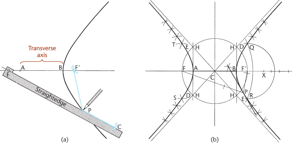
Fasten the straightedge at F. If it is revolved about F, with the pencil point moving against it and with the string taut, the hyperbola may be drawn as shown.
To construct the curve geometrically, select any point X on the transverse axis produced (Figure A52.6b). With centers at F and F′ and BX as radius, draw the arcs DE. With the same centers, F and F′, and AX as radius, draw arcs to intersect the arcs first drawn through the points Q, R, S, and T, which are points of the required hyperbola. Find as many additional points as are necessary to draw the curves accurately by selecting other points similar to point X along the transverse axis and proceeding as described for point X.
To draw the tangent to a hyperbola at a given point P, bisect the angle between the focal radii FP and F′P. The bisector is the required tangent.
To draw the asymptotes HCH of the hyperbola, draw a circle with the diameter FF′ and draw perpendiculars to the transverse axis at points A and B to intersect the circle at points H. The lines HCH are the required asymptotes.
Drawing an Equilateral Hyperbola
Asymptotes OB and OA, at right angles to each other, and point P on the curve are given (Figure A52.7).

In an equilateral hyperbola, the asymptotes, which are at right angles to each other, may be used as the axes to which the curve is referred. If a chord of the hyperbola is extended to intersect the axes, the intercepts between the curve and the axes are equal (Figure A52.7a). For example, a chord through given point P intersects the axes at points 1 and 2, intercepts P–1 and 2–3 are equal, and point 3 is a point on the hyperbola. Likewise, another chord through P provides equal intercepts P–1′ and 3′–2′, and point 3′ is a point on the curve. Not all chords need be drawn through given point P, but as new points are established on the curve, chords may be drawn through them to obtain more points. After finding enough points to ensure an accurate curve, draw the hyperbola with the aid of an irregular curve.
In an equilateral hyperbola, the coordinates are related, so their products remain constant. Through given point P, draw lines 1–P–Y and 2–P–Z parallel, respectively, to the axes (Figure A52.7b). From coordinate O, draw any diagonal intersecting these two lines at points 3 and X. At these points draw lines parallel to the axes, intersecting at point 4, a point on the curve. Likewise, another diagonal from O intersects the two lines through P at points 8 and Y, and lines through these points parallel to the axes intersect at point 9, another point on the curve. A third diagonal similarly produces point 10 on the curve, and so on. Find as many points as necessary for a smooth curve, and draw the hyperbola with the aid of an irregular curve. From the similar triangles O–X–5 and O–3–2, it is evident that lines P–1 × P–2 = 4–5 × 4–6.
The equilateral hyperbola can be used to represent varying pressure of a gas as the volume varies, because the pressure varies inversely with the volume; that is, pressure × volume is constant.
Drawing a Spiral of Archimedes
To find points on the curve, draw lines through the pole C, making equal angles with each other, such as 30° angles (Figure A52.8). Beginning with any one line, set off any distance, such as 2 mm or 1/16″, set off twice that distance on the next line, three times on the third, and so on. Use an irregular curve to draw a smooth curve.

Drawing a Helix
A helix is generated by a point moving around and along the surface of a cylinder or cone with a uniform angular velocity and a uniform linear velocity about the axis, and with a uniform velocity in the direction of the axis (Figure A52.9). A cylindrical helix is simply known as a helix. The distance measured parallel to the axis traversed by the point in one revolution is called the lead.

If the cylindrical surface on which a helix is generated is rolled out onto a plane, the helix becomes a straight line (Figure A52.9a). The portion below the helix becomes a right triangle, the altitude of which is equal to the lead of the helix; the length of the base is equal to the circumference of the cylinder. Such a helix can be defined as the shortest line that can be drawn on the surface of a cylinder connecting two points not on the same element.
To draw the helix, draw two views of the cylinder on which the helix is generated (Figure A52.9b). Divide the circle of the base into any number of equal parts. On the rectangular view of the cylinder, set off the lead and divide it into the same number of equal parts as the base. Number the divisions as shown (in this case 16). When the generating point has moved one sixteenth of the distance around the cylinder, it will have risen one sixteenth of the lead; when it has moved halfway around the cylinder, it will have risen half the lead; and so on. Points on the helix are found by projecting up from point 1 in the circular view to line 1 in the rectangular view, from point 2 in the circular view to line 2 in the rectangular view, and so on.
Figure A52.9b is a right-handed helix. In a left-handed helix (Figure A52.9c), the visible portions of the curve are inclined in the opposite direction—that is, downward to the right. The helix shown in Figure A52.9b can be converted into a left-handed helix by interchanging the visible and hidden lines.
The helix is used in industry, as in screw threads, worm gears, conveyors, spiral stairways, and so on. The stripes of a barber pole are helical in form.
The construction for a right-handed conical helix is shown in Figure A52.9d.
Drawing an Involute
An involute is the path of a point on a string as the string unwinds from a line, polygon, or circle.
To Draw an Involute of a Line
Let AB be the given line. With AB as radius and B as center, draw the semicircle AC (Figure A52.10a). With AC as radius and A as center, draw the semicircle CD. With BD as radius and B as center, draw the semicircle DE. Continue similarly, alternating centers between A and B, until the figure is completed.

To Draw an Involute of a Triangle
Let ABC be the given triangle. With CA as radius and C as center, draw arc AD (Figure A52.10b). With BD as radius and B as center, draw arc DE. With AE as radius and A as center, draw arc EF. Continue similarly until the figure is completed.
To Draw an Involute of a Square
Let ABCD be the given square. With DA as radius and D as center, draw the 90° arc AE (Figure A52.10c). Proceed as for the involute of a triangle until the figure is completed.
To Draw an Involute of a Circle
A circle may be considered a polygon with an infinite number of sides (Figure A52.10d). The involute is constructed by dividing the circumference into a number of equal parts, drawing a tangent at each division point, setting off along each tangent the length of the corresponding circular arc (Figure A52.10c), and drawing the required curve through the points set off on the several tangents.
An involute can be generated by a point on a straight line that is rolled on a fixed circle (Figure A52.10e). Points on the required curve may be determined by setting off equal distances 0–1, 1–2, 2–3, and so on, along the circumference, drawing a tangent at each division point, and proceeding as explained for Figure A52.10d.
The involute of a circle is used in the construction of involute gear teeth. In this system, the involute forms the face and a part of the flank of the teeth of gear wheels; the outlines of the teeth of racks are straight lines.
Drawing a Cycloid
A cycloid is generated by a point P on the circumference of a circle that rolls along a straight line (Figure A52.11).

Given the generating circle and the straight line AB tangent to it, make both distances CA and CB equal to the semicircumference of the circle (see Figure A52.11). Divide these distances and the semicircumference into the same number of equal parts (six, for instance) and number them consecutively, as shown. Suppose the circle rolls to the left; when point 1 of the circle reaches point 1′ of the line, the center of the circle will be at D, point 7 will be the highest point of the circle, and the generating point 6 will be at the same distance from line AB as point 5 is when the circle is in its central position. To find point P′, draw a line through point 5 parallel to AB and intersect it with an arc drawn from the center D with a radius equal to that of the circle. To find point P″, draw a line through point 4 parallel to AB, and intersect it with an arc drawn from the center E, with a radius equal to that of the circle. Points J, K, and L are found in a similar way.
Another method is shown in the right half of Figure A52.11. With the center at 11′ and the chord 11–6 as radius, draw an arc. With 10′ as center and the chord 10–6 as radius, draw an arc. Continue similarly with centers 9′, 8′, and 7′. Draw the required cycloid tangent to these arcs.
Either method may be used; however, the second is shorter. The line joining the generating point and the point of contact for the generating circle is a normal of the cycloid. The lines 1′–P′ and 2′–P″, for instance, are normals; this property makes the cycloid suitable for the outlines of gear teeth.
Drawing an Epicycloid or a Hypocycloid
If the generating point P is on the circumference of a circle that rolls along the convex side of a larger circle, the curve generated is an epicycloid (Figure A52.12a). If the circle rolls along the concave side of a larger circle, the curve generated is a hypocycloid (Figure A52.12b). These curves are drawn in much the same way as the cycloid (Figure A52.11). Like cycloids, these curves are used to form the outlines of certain gear teeth and are therefore of practical importance in machine design.
