
Chapter 1. Fundamentals of Networking Protocols and Networking Devices
This chapter covers the following topics:
![]() Introduction to TCP/IP and OSI models
Introduction to TCP/IP and OSI models
![]() Wired LAN and Ethernet
Wired LAN and Ethernet
![]() Frame switching
Frame switching
![]() Hub, switch, and router
Hub, switch, and router
![]() Wireless LAN and technologies
Wireless LAN and technologies
![]() Wireless LAN controller and access point
Wireless LAN controller and access point
![]() IPv4 and IPv6 addressing
IPv4 and IPv6 addressing
![]() IP routing
IP routing
![]() ARP, DHCP, ICMP, and DNS
ARP, DHCP, ICMP, and DNS
![]() Transport layer protocols
Transport layer protocols
Welcome to the first chapter of the CCNA Cyber Ops SECFND #210-250 Official Cert Guide. In this chapter, we go through the fundamentals of networking protocols and explore how devices such as switches and routers work to allow two hosts to communicate with each other, even if they are separated by many miles.
If you are already familiar with these topics—for example, if you already have a CCNA Routing and Switching certification—this chapter will serve as a refresher on protocols and device operations. If, on the other hand, you are approaching these topics for the first time, you’ll learn about the fundamental protocols and devices at the base of Internet communication and how they work.
This chapter begins with an introduction to the TCP/IP and OSI models and then explores link layer technologies and protocols—specifically the Ethernet and Wireless LAN technologies. We then discuss how the Internet Protocol (IP) works and how a router uses IP to move packets from one site to another. Finally, we look into the two most used transport layer protocols: Transmission Control Protocol (TCP) and User Datagram Protocol (UDP).
“Do I Know This Already?” Quiz
The “Do I Know This Already?” quiz helps you identify your strengths and deficiencies in this chapter’s topics. The 13-question quiz, derived from the major sections in the “Foundation Topics” portion of the chapter, helps you determine how to spend your limited study time. You can find the answers in Appendix A Answers to the “Do I Know This Already?” Quizzes and Q&A Questions.
Table 1-1 outlines the major topics discussed in this chapter and the “Do I Know This Already?” quiz questions that correspond to those topics.
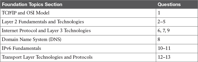
Table 1-1 “Do I Know This Already?” Section-to-Question Mapping
1. Which layer of the TCP/IP model is concerned with end-to-end communication and offers multiplexing service?
a. Transport
b. Internet
c. Link layer
d. Application
2. Which statement is true concerning a link working in Ethernet half-duplex mode?
a. A collision cannot happen.
b. When a collision happens, the two stations immediately retransmit.
c. When a collision happens, the two stations wait for a random time before retransmitting.
d. To avoid a collision, stations wait a random time before transmitting.
3. What is the main characteristic of a hub?
a. It regenerates the signal and retransmits on all ports.
b. It uses a MAC address table to switch frames.
c. When a packet arrives, the hub looks up the routing table before forwarding the packet.
d. It supports full-duplex mode of transmission.
4. Where is the information about ports and device Layer 2 addresses kept in a switch?
a. MAC address table
b. Routing table
c. L2 address table
d. Port table
5. Which of the following features are implemented by a wireless LAN controller? (Select all that apply.)
a. Wireless station authentication
b. Quality of Service
c. Channel encryption
d. Transmission and reception of frames
6. Which IP header field is used to recognize fragments from the same packet?
a. Identification
b. Fragment Offset
c. Flags
d. Destination Address
7. Which protocol is used to request a host MAC address given a known IP address?
a. ARP
b. DHCP
c. ARPv6
d. DNS
8. Which type of query is sent from a DNS resolver to a DNS server?
a. Recursive
b. Iterative
c. Simple
d. Type Q query
9. How many host IPv4 addresses are possible in a /25 network?
a. 126
b. 128
c. 254
d. 192
10. How many bits can be used for host IPv6 addresses assignment in the 2345::/64 network?
a. 48
b. 64
c. 16
d. 264
11. What is SLAAC used for?
a. To provide an IPv6 address to a client
b. To route IPv6 packets
c. To assign a DNS server
d. To provide a MAC address given an IP address
12. Which one of these protocols requires a connection to be established before transmitting data?
a. TCP
b. UDP
c. IP
d. OSPF
13. What is the TCP window field used for?
a. Error detection
b. Flow control
c. Fragmentation
d. Multiplexing
Foundation Topics
TCP/IP and OSI Model
Two main models are currently used to explain the operation of an IP-based network. These are the TCP/IP model and the Open System Interconnection (OSI) model. This section provides an overview of these two models.
TCP/IP Model
The TCP/IP model is the foundation for most of the modern communication networks. Every day, each of us uses some application based on the TCP/IP model to communicate. Think, for example, about a task we consider simple: browsing a web page. That simple action would not be possible without the TCP/IP model.
The TCP/IP model’s name includes the two main protocols we will discuss in the course of this chapter: Transmission Control Protocol (TCP) and Internet Protocol (IP). However, the model goes beyond these two protocols and defines a layered approach that can map nearly any protocol used in today’s communication.
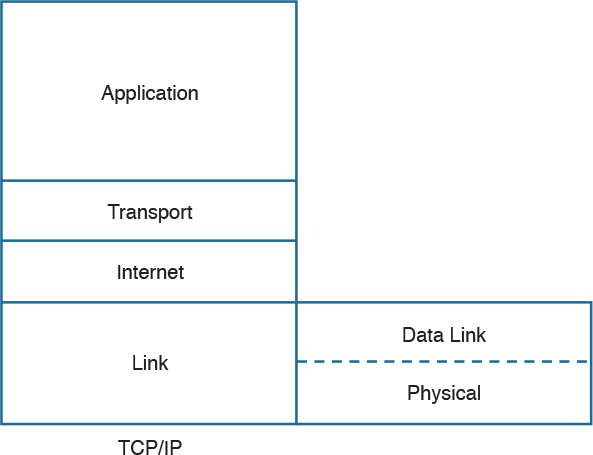
In its original definition, the TCP/IP model included four layers, where each of the layers would provide transmission and other services for the level above it. These are the link layer, internet layer, transport layer, and application layer.
In its most modern definition, the link layer is split into two additional layers to clearly demark the physical and data link type of services and protocols included in this layer. Internet layer is also sometimes called the networking layer, which is based on another very known model, the OSI model, which is described in the next section. Figure 1-1 shows the TCP/IP stack model.
The TCP/IP model works on two main concepts that define how the layers interact:
![]() On the same host, each layer works by providing services for the layer above it on the TCP/IP stack.
On the same host, each layer works by providing services for the layer above it on the TCP/IP stack.
![]() On different hosts, a same layer communication is established by using the same layer protocol.
On different hosts, a same layer communication is established by using the same layer protocol.
For example, on your personal computer, the TCP/IP stack is implemented to allow networking communication. The link layer provides services for the IP layer (for example, encapsulation of an IP packet in an Ethernet frame). The IP layer provides services to the transport layer (for example, IP routing and IP addressing), and so on. These are all examples of services provided to the layer above it within the host.
Now imagine that your personal computer wants to connect to a web server (for example, to browse a web page). The web server will also implement the TCP/IP stack. In this case, the IP layer of your personal computer and the IP layer of the web server will use a common protocol, IP, for the communication. The same thing will happen with the transport protocol, where the two devices will use TCP, and so on. These are examples of the same layer protocol used on different hosts to communicate.
Later in this chapter, the “Networking Communication with the TCP/IP Model,” section provides more detail about how the communication works between two hosts and how the TCP/IP stack is used on the same host.
The list that follows analyzes each layer in a bit more detail:
![]() Link layer: The link layer provides physical transmission support and includes the protocols used to transmit information over a link between two devices. In simple terms, the link layer includes the hardware and protocol necessary to send information between two hosts that are connected by a physical link (for example, a cable) or over the air (for example, via radio waves). It also includes the notion of and mechanisms for information being replicated and retransmitted over several ports or links by dedicated devices such as switches and bridges.
Link layer: The link layer provides physical transmission support and includes the protocols used to transmit information over a link between two devices. In simple terms, the link layer includes the hardware and protocol necessary to send information between two hosts that are connected by a physical link (for example, a cable) or over the air (for example, via radio waves). It also includes the notion of and mechanisms for information being replicated and retransmitted over several ports or links by dedicated devices such as switches and bridges.
Because different physical means are used to transmit information, there are several protocols that work at the link layer. One of the most popular is the Ethernet protocol. As mentioned earlier, nowadays the link layer is usually split further in the physical layer, which is concerned about physical bit transmission, and the data link layer, which provides encapsulation and addressing facilities as well as abstraction for the upper layers.
At link layer, the message unit is called a frame.
![]() Internet layer: Of course, not all devices can be directly connected to each other, so there is a need to transmit the information across multiple devices. The Internet layer provides networking services and includes protocols that allow for the transmission of information through multiple hops. To do that, each host is identified by an Internet Protocol (IP) address, or a different address if another Internet Protocol type is used. Each hop device between two hosts, called networking nodes, knows how to reach the destination IP address and transmit the information to the next best node to reach the destination. The nodes are said to perform the routing of the information, and the way each node, also called router, determines the best next node to the destination is called the routing protocol.
Internet layer: Of course, not all devices can be directly connected to each other, so there is a need to transmit the information across multiple devices. The Internet layer provides networking services and includes protocols that allow for the transmission of information through multiple hops. To do that, each host is identified by an Internet Protocol (IP) address, or a different address if another Internet Protocol type is used. Each hop device between two hosts, called networking nodes, knows how to reach the destination IP address and transmit the information to the next best node to reach the destination. The nodes are said to perform the routing of the information, and the way each node, also called router, determines the best next node to the destination is called the routing protocol.
At the Internet layer, the message unit is called a packet.
![]() Transport layer: When transmitting information, the sending host knows when the information is sent, but has no way to know whether it actually made it to the destination. The transport layer provides services to successfully transfer information between two end points. It abstracts the lower-level layer and is concerned about the end-to-end process. For example, it is used to detect whether any part of the information went missing. It also provides information about which type of information is being transmitted. For example, a host may want to request a web page and also start an FTP transaction. How do we distinguish between these two actions? The transport layer helps to separate the two requests by using the concept of a transport layer port. Each service is enabled on a different transport layer port—for example, port 80 for a web request or port 21 for an FTP transaction. So when the destination host receives a request on port 80, it knows that this needs to be passed to the application layer handling web requests. This type of service provided by the transport layer is called multiplexing.
Transport layer: When transmitting information, the sending host knows when the information is sent, but has no way to know whether it actually made it to the destination. The transport layer provides services to successfully transfer information between two end points. It abstracts the lower-level layer and is concerned about the end-to-end process. For example, it is used to detect whether any part of the information went missing. It also provides information about which type of information is being transmitted. For example, a host may want to request a web page and also start an FTP transaction. How do we distinguish between these two actions? The transport layer helps to separate the two requests by using the concept of a transport layer port. Each service is enabled on a different transport layer port—for example, port 80 for a web request or port 21 for an FTP transaction. So when the destination host receives a request on port 80, it knows that this needs to be passed to the application layer handling web requests. This type of service provided by the transport layer is called multiplexing.
At this layer, the message unit is called a segment.
![]() Application layer: The application layer is the top layer and is the one most familiar to end users. For example, at the application layer, a user may use the email client to send an email message or use a web browser to browse a website. Both of these actions map to a specific application, which uses a protocol to fulfill the service.
Application layer: The application layer is the top layer and is the one most familiar to end users. For example, at the application layer, a user may use the email client to send an email message or use a web browser to browse a website. Both of these actions map to a specific application, which uses a protocol to fulfill the service.
In this example, the Simple Message Transfer Protocol (SMTP) is used to handle the email transfer, whereas the Hypertext Transfer Protocol (HTTP) is used to request a web page within a browser. At this level, the protocols are not concerned with how the information will reach the destination, but only work on defining the content of the information being transmitted.
Table 1-2 shows examples of protocols working at each layer of the TCP/IP model.
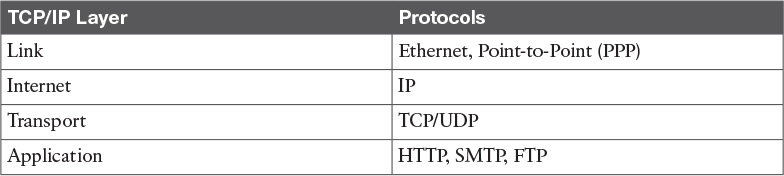
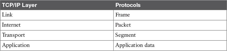
Table 1-3 summarizes what message units are referred to as at each layer.
TCP/IP Model Encapsulation
In the TCP/IP model, each layer provides services for the level above it. Protocols at each layer include a protocol header and in some cases a trailer to the information provided by the upper layer. The protocol header includes enough information for the protocol to work toward the delivery of the information. This process is called encapsulation.
When the information arrives to the destination, the inverse process is used. Each layer reads the information present in the header of the protocol working at that specific layer, performs an action based on that information, and, if needed, passes the remaining information to the next layer in the stack. This process is called decapsulation.
Figure 1-2 shows an example of encapsulation.
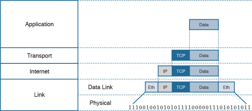
Referring to Figure 1-2, let’s assume that this represents the TCP/IP stack of a host, for example Host A, trying to request a web page using HTTP. Let’s see how the encapsulation works, step by step:
Step 1. In this example, the host has requested a web page using the HTTP application layer protocol. The HTTP application generates the information, represented as HTTP “data” in this example.
Step 2. On the host, the TCP/IP implementation would detect that HTTP uses TCP at the transport layer and will send the HTTP data to the transport layer for further handling. The protocol at the transport layer, TCP, will create a TCP header, which includes information such as the service port (TCP port 80 for a web page request), and will send it to the next layer, the Internet layer, for further processing. The TCP header plus the payload forms a TCP segment.
Step 3. The Internet layer receives the TCP information, attaches an IP header, and encapsulates it in an IP packet. The IP header will contain information to handle the packet at the Internet layer. This includes, for example, the IP addresses of the source and destination.
Step 4. The IP packet is then passed to the link layer for further processing. The TCP/IP stack detects that it needs to use Ethernet to transmit the frame to the next device. It will add an Ethernet header and trailer and transmit the frame to the physical network interface card (NIC), which will take care of the physical transmission of the frame.
When the information arrives to the destination, the receiving host will start from the bottom of the TCP/IP stack by receiving an Ethernet frame. The link layer of the destination host will read and process the header and trailer, and then pass the IP packet to the Internet layer for further processing.
The same process happens at the Internet layer, and the TCP segment is passed to the transport layer, which will again process the TCP header information and pass the HTTP data for final processing to the HTTP application.
Networking Communication with the TCP/IP Model
Let’s look back at the example of browsing a web page and see how the TCP/IP model is used to transmit and receive information through a networking connection path.
A networking device is a device that implements the TCP/IP model. The model may be fully implemented (for example, in the case of a user computer or a server) or partially implemented (for example, a router might implement the TCP/IP stack only up to the Internet layer).
Figure 1-3 shows the logical topology. It includes two hosts: Host A, which is requesting a web page, and Server B, which is the destination of the request. The network connectivity is provided by two routers: R1 and R2, which are connected via an optical link. The host and server are directly connected to R1 and R2, respectively, with a physical cable.
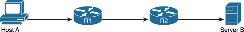
Figure 1-4 shows how each TCP/IP model layer interacts in this case.
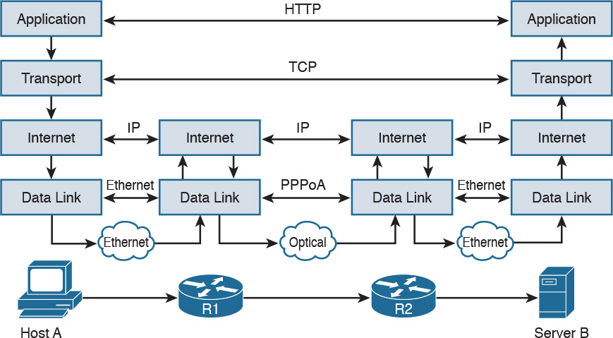
Referring to Figure 1-4, let’s see how the steps are executed:
Step 1. The HTTP application on Host A will create an HTTP Application message that includes an HTTP header and the contents of the request in the payload. This will be encapsulated up to the link layer, as described in Figure 1-2, and transmitted over the cable to R1.
Step 2. The R1 link layer will receive the frame, extract the IP packet, and send it to the IP layer. Because the main function of the router is to forward the IP packet, it will not further decapsulate the packet. It will use the information in the IP header to forward the packet to the best next router, R2. To do that, it will encapsulate the IP packet in a new link layer frame—for example, Point-to-Point over ATM (PPPoA)—and send the frame on the physical link toward R2.
Step 3. R2 will follow the same process that R1 followed in step 2 and will send the IP packet encapsulated in a new Ethernet frame to Host B.
Step 4. Server B’s link layer will decapsulate the frame and send it to the Internet layer.
Step 5. The Internet layer detects that the packet is destined to Server B itself by looking into the IP header information (more specifically the value of the destination IP address). It strips the IP header and passes the TCP segment to the transport layer.
Step 6. The transport layer uses the port information included in the TCP header to determine to which application to pass the data (in this case, the web service application).
Step 7. The application layer, the web service, finally receives the request and may decide to respond (for example, by providing the web page to Host A). The process will start again, with the web service creating some data and passing it to the HTTP application layer protocol for handling.
The example in Figure 1-4 is very simplistic. For example, TCP requires a connection to be established before transmitting data. However, it is important that the main idea behind the TCP/IP model is clear as a basis for understanding how the various protocols work.
Open System Interconnection Model
The Open System Interconnection (OSI) reference model is another model that uses abstraction layers to represent the operation of communication systems. The idea behind the design of the OSI model is to be comprehensive enough to take into account advancement in network communications and to be general enough to allow several existing models for communication systems to transition to the OSI model.
The OSI model presents several similarities with the TCP/IP model described in the previous section. One of the most important similarities is the use of abstraction layers. As with TCP/IP, each layer provides service for the layer above it within the same computing device, while it interacts at the same layer with other computing devices.
The OSI model includes seven abstract layers, each representing a different function and service within a communication network:
![]() Physical layer—Layer 1 (L1): Provides services for the transmission of bits over the data link.
Physical layer—Layer 1 (L1): Provides services for the transmission of bits over the data link.
![]() Data link layer—Layer 2 (L2): Includes protocols and functions to transmit information over a link between two connected devices. For example, it provides flow control and L1 error detection.
Data link layer—Layer 2 (L2): Includes protocols and functions to transmit information over a link between two connected devices. For example, it provides flow control and L1 error detection.
![]() Network layer—Layer 3 (L3): This layer includes the function necessary to transmit information across a network and provides abstraction on the underlying means of connection. It defines L3 addressing, routing, and packet forwarding.
Network layer—Layer 3 (L3): This layer includes the function necessary to transmit information across a network and provides abstraction on the underlying means of connection. It defines L3 addressing, routing, and packet forwarding.
![]() Transport layer—Layer 4 (L4): This layer includes services for end-to-end connection establishment and information delivery. For example, it includes error detection, retransmission capabilities, and multiplexing.
Transport layer—Layer 4 (L4): This layer includes services for end-to-end connection establishment and information delivery. For example, it includes error detection, retransmission capabilities, and multiplexing.
![]() Session layer—Layer 5 (L5): This layer provides services to the presentation layer to establish a session and exchange presentation layer data.
Session layer—Layer 5 (L5): This layer provides services to the presentation layer to establish a session and exchange presentation layer data.
![]() Presentation layer—Layer 6 (L6): This layer provides services to the application layer to deal with specific syntax, which is how data is presented to the end user.
Presentation layer—Layer 6 (L6): This layer provides services to the application layer to deal with specific syntax, which is how data is presented to the end user.
![]() Application layer—Layer 7 (L7): This is the last (or first) layer of the OSI model (depending on how you see it). It includes all the services of a user application, including the interaction with the end user.
Application layer—Layer 7 (L7): This is the last (or first) layer of the OSI model (depending on how you see it). It includes all the services of a user application, including the interaction with the end user.
The functionalities of the OSI layers can be mapped to similar functionalities provided by the TCP/IP model. It is sometimes common to use OSI layer terminology to indicate a protocol operating at a specific layer, even if the communication device implements the TCP/IP model instead of the OSI model.
Figure 1-5 shows how each layer of the OSI model maps to the corresponding TCP/IP layer.
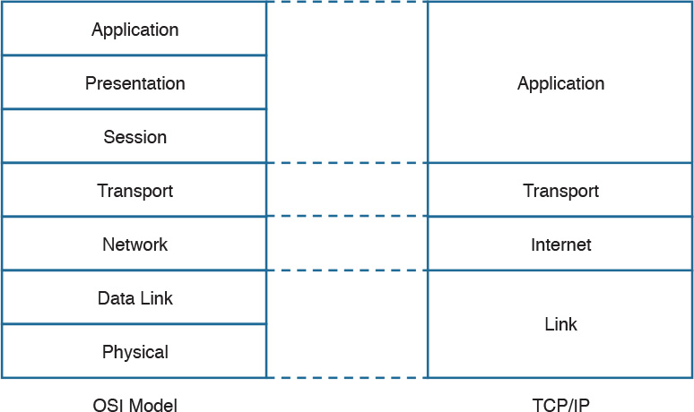
The physical and data link layers of the OSI model provide the same functions as the link layer in the TCP/IP model. The network layer can be mapped to the Internet layer, and the transport layer in OSI provides similar services as the transport layer in TCP/IP. The OSI session, presentation, and application layers map to the TCP/IP application layer.
Within the same host, each layer interacts with the adjacent layer in a way that is similar to the encapsulation performed in the TCP/IP model. The encapsulation is formalized in the OSI model as follows:
![]() Protocol control information (PCI) for a layer (N) is the information added by the protocol.
Protocol control information (PCI) for a layer (N) is the information added by the protocol.
![]() A protocol data unit (PDU) for a layer (N) is composed by the data produced at that layer plus the PCI for that layer.
A protocol data unit (PDU) for a layer (N) is composed by the data produced at that layer plus the PCI for that layer.
![]() A service data unit (SDU) for a layer (N) is the (N+1) layer PDU.
A service data unit (SDU) for a layer (N) is the (N+1) layer PDU.
Figure 1-6 shows the relationship between PCI, PDU, and SDU.
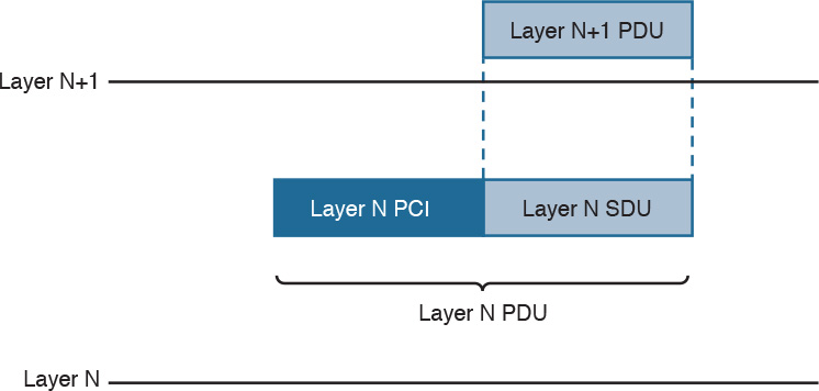
For example, a TCP segment includes the TCP header, which maps to the L4PCI and a TCP payload, including the data to transmit. Together, they form a L4PDU. When the L4PDU is passed to the networking layer (for example, to be processed by IP), the L4PDU is the same as the L3SDU. IP will add an IP header, the L3PCI. The L3PCI plus the L3SDU will form the L3PDU, and so on.
The encapsulation process works in a similar way to the TCP/IP model. Each layer protocol adds its own protocol header and passes the information to the lower-layer protocol.
Figure 1-7 shows an example of encapsulation in the OSI model.
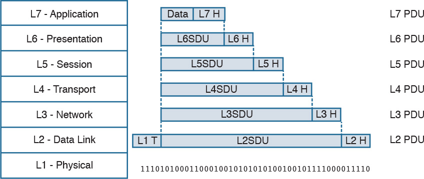
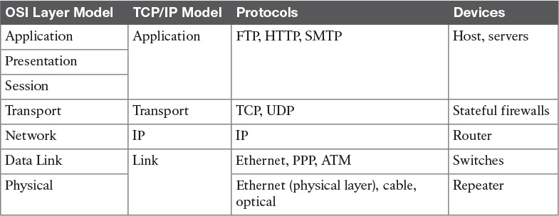
Table 1-4 shows examples of protocols and devices that work at a specific OSI layer. Note that each device is mapped to a level related to its main function capability. For example, a router’s main function is forwarding packets based on L3 information, so it is usually referred to as an L3 device; however, it also needs to incorporate L2 and L1 functionalities. Furthermore, a router may implement the full OSI model (for example, because it implements some additional features such as firewalling or VPN). The same rationale could be applied to firewalls. They are usually classified as L4 devices; however, most of the time they are able to inspect traffic up to the application layer.
The flow of information through a network in the OSI model is similar to what’s described in Figure 1-4 for the TCP/IP model. This is not by chance, because the OSI model has been designed to offer compatibility and enable the transition to the OSI model from multiple other communication models (for example, from TCP/IP).
Figure 1-8 shows a network implementing the OSI model.
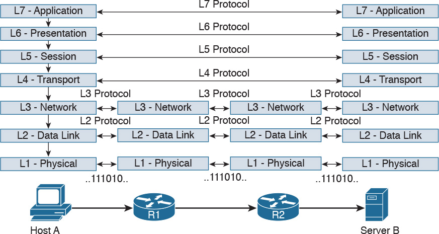
In the rest of this book, we will use the OSI model and TCP/IP model layer names interchangeably.
Layer 2 Fundamentals and Technologies
This section goes through the fundamentals of the link layer (or Layer 2). Although it is not required to know specific implementations and configurations, the CCNA Cyber Ops SECFND exam requires candidates to understand the various link layer technologies, such as hubs, bridges, and switches, and their behavior. Candidates also need to understand the protocols that enable the link layer communication. Readers interested in learning more about Layer 2 technologies and protocols can refer to CCNA Routing and Switching materials for more comprehensive information on the topic.
Two very well-known concepts used to describe communication networks at Layer 2 are local area network (LAN) and wide area network (WAN). As the names suggest, a LAN is a collection of devices, protocols, and technologies operating nearby each other, whereas a WAN typically deals with devices, protocols, and technologies used to transmit information over a long distance.
The next sections introduce two of the most used LAN types: wired LANs (specifically Ethernet-based LANs) and wireless LANs.
Ethernet LAN Fundamentals and Technologies
Ethernet is a protocol used to provide transmission and services for the physical and data link layers, and it is described in the IEEE 802.3 standards collection. Ethernet is part of the larger IEEE 802 standards for LAN communication. Another example of the IEEE 802 standards is 802.11, which covers wireless LAN.
The Ethernet collection includes standards specifying the functionality at the physical layer and data link layer. The Ethernet physical layer includes several standards, depending on the physical means used to transmit the information. The data link layer functionality is provided by the Ethernet Medium Access Control (MAC) described in IEEE 802.3, together with the Logical Link Control (LLC) described in IEEE 802.2.
Note that MAC is sometimes referred to as Media Access Control instead of Medium Access Control. Both ways are correct according to the IEEE 802. In the rest of this document we will use Medium Access Control or simply MAC.
LLC was initially used to allow several types of Layer 3 protocols to work with the MAC. However, in most networks in use today, there is only one type of Layer 3 protocol, which is the Internet Protocol (IP), so LLC is seldom used because IP can be directly encapsulated using MAC.
The following sections provide an overview of the Ethernet physical layer and MAC layer standards.
Ethernet Physical Layer
The physical layer includes several standards to account for the various physical means possibly encountered in a LAN deployment. For example, the transmission can happen over an optical fiber, copper, and so on.
Examples of Ethernet standards are 10BASE-T and 1000BASE-LX. Each Ethernet standard is characterized by the maximum transmission speed and maximum distance between two connected stations. Specifically, the transmission speed has seen (and is currently seeing) the biggest evolution.
Table 1-5 shows examples of popular Ethernet physical layer standards.
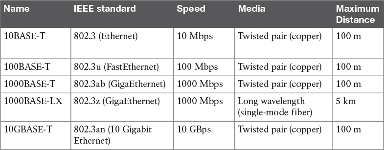
The Ethernet nomenclature is easy to understand. Each standard name follows this format:
sTYPE-M
where:
![]() s: The speed (for example, 1000).
s: The speed (for example, 1000).
![]() TYPE: The modulation type (for example, baseband [BASE]).
TYPE: The modulation type (for example, baseband [BASE]).
![]() M: The information about the medium. Examples include T for twisted pair, F for fiber, L for long wavelength, and X for external sourced coding.
M: The information about the medium. Examples include T for twisted pair, F for fiber, L for long wavelength, and X for external sourced coding.
For example, with 1000BASE-T, the speed is 1000, the modulation is baseband, and the medium (T) is twisted-pair cable (copper).
An additional characteristic of a physical Ethernet standard is the type of cable and connector used to connect two stations. For example, 1000BASE-T would need a Category 6 (CAT 6) unshielded twisted-pair cable (UTP) and RJ-45 connectors.
Ethernet Medium Access Control
Ethernet MAC deals with the means used to transfer information between two Ethernet devices, also called stations, and it is independent from the physical means used for transmission.
The standard describes two modes of medium access:
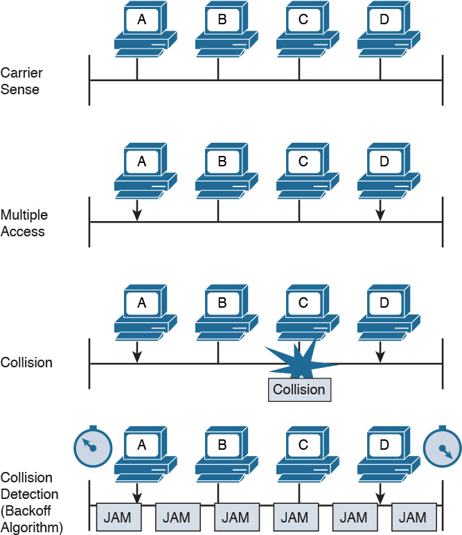
![]() Half duplex: In half-duplex mode, two Ethernet devices share a common transmission medium. The access is controlled by implementing Carrier Sense Multiple Access with Collision Detection (CSMA/CD). In CSMA/CD, a device has the ability to detect whether there is a transmission occurring over the shared medium. When there is no transmission, a device can start sending. It can happen that two devices send nearly at the same time. In that case, there is a message collision. When a collision occurs, it is detected by CSMA/CD-enabled devices, which will then stop transmitting and will delay the transmission for a certain amount of time, called the backoff time. The jam signal is used by the station to signal that a collision occurred. All stations that can sense a collision are said to be in the same collision domain.
Half duplex: In half-duplex mode, two Ethernet devices share a common transmission medium. The access is controlled by implementing Carrier Sense Multiple Access with Collision Detection (CSMA/CD). In CSMA/CD, a device has the ability to detect whether there is a transmission occurring over the shared medium. When there is no transmission, a device can start sending. It can happen that two devices send nearly at the same time. In that case, there is a message collision. When a collision occurs, it is detected by CSMA/CD-enabled devices, which will then stop transmitting and will delay the transmission for a certain amount of time, called the backoff time. The jam signal is used by the station to signal that a collision occurred. All stations that can sense a collision are said to be in the same collision domain.
Half-duplex mode was used in early implementations of Ethernet; however, due to several limitations, including transmission performance, it is rarely seen nowadays. A network hub is an example of a device that can be used to share a common transmission medium across multiple Ethernet stations. You’ll learn more about hubs later in this chapter in the “LAN Hubs and Bridges” section.
Figure 1-9 shows an example of CSMA/CD access.
![]() Full duplex: In full-duplex mode, two devices can transmit simultaneously because there is a dedicated channel allocated for the transmission. Because of that, there is no need to detect collisions or to wait before transmitting. Full duplex is called “collision free” because collisions cannot happen.
Full duplex: In full-duplex mode, two devices can transmit simultaneously because there is a dedicated channel allocated for the transmission. Because of that, there is no need to detect collisions or to wait before transmitting. Full duplex is called “collision free” because collisions cannot happen.
A switch is an example of a device that provides a collision-free domain and dedicated transmission channel. You’ll learn more about switches later in this chapter in the “LAN Switches” section.
Ethernet Frame
Figure 1-10 shows an example of an Ethernet frame.
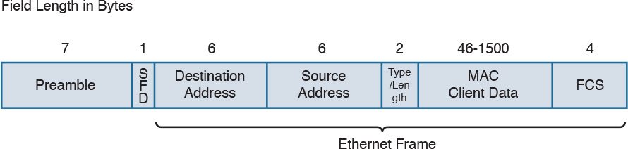
The Ethernet frame includes the following fields:
![]() Preamble: Used for the two stations for synchronization purposes.
Preamble: Used for the two stations for synchronization purposes.
![]() Start Frame Delimiter (SFD): Indicates the start of the Ethernet frame. This is always set to 10101011.
Start Frame Delimiter (SFD): Indicates the start of the Ethernet frame. This is always set to 10101011.
![]() Destination Address: Contains the recipient address of the frame.
Destination Address: Contains the recipient address of the frame.
![]() Source Address: Contains the source of the frame.
Source Address: Contains the source of the frame.
![]() Length/Type: This field can contain either the length of the MAC Client Data (length interpretation) or the type code of the Layer 3 protocol transported in the frame payload (type interpretation). The latter is the most common. For example, code 0800 indicates IPv4, and code 08DD indicates IPv6.
Length/Type: This field can contain either the length of the MAC Client Data (length interpretation) or the type code of the Layer 3 protocol transported in the frame payload (type interpretation). The latter is the most common. For example, code 0800 indicates IPv4, and code 08DD indicates IPv6.
![]() MAC Client Data and Pad: This field contains information being encapsulated at the Ethernet layer (for example, an LLC PDU or an IP packet). The minimum length is 46 bytes; the maximum length depends on the type of Ethernet frame:
MAC Client Data and Pad: This field contains information being encapsulated at the Ethernet layer (for example, an LLC PDU or an IP packet). The minimum length is 46 bytes; the maximum length depends on the type of Ethernet frame:
![]() 1500 bytes for basic frames. This is the most common Ethernet frame.
1500 bytes for basic frames. This is the most common Ethernet frame.
![]() 1504 bytes for Q-tagged frames.
1504 bytes for Q-tagged frames.
![]() 1982 bytes for envelope frames.
1982 bytes for envelope frames.
![]() Frame Check Sequence (FCS): This field is used by the receiving device to detect errors in transmission. This is usually called the Ethernet trailer. Optionally, an additional extension may be present.
Frame Check Sequence (FCS): This field is used by the receiving device to detect errors in transmission. This is usually called the Ethernet trailer. Optionally, an additional extension may be present.
Ethernet Addresses
To transmit a frame, Ethernet uses source and destination addresses. The Ethernet addresses are called MAC addresses, or Extended Unique Identifier (EUI) in the new terminology, and they are either 48 bits (MAC-48 or EUI-48) or 64 bits (MAC-64 or EUI-64), if we consider all MAC addresses for the larger IEEE 802 standard.
The MAC address is usually expressed in hexadecimal. There are few ways it can be written for easier reading. The following two ways are the ones used the most:
![]() 01-23-45-67-89-ab (IEEE 802)
01-23-45-67-89-ab (IEEE 802)
![]() 0123.4567.89ab (Cisco notation)
0123.4567.89ab (Cisco notation)
There are three types of MAC addresses:
![]() Broadcast: A broadcast MAC address is obtained by setting all 1s in the MAC address field. This results in an address like FFFF.FFFF.FFFF. A frame with a broadcast destination address is transmitted to all the devices within a LAN.
Broadcast: A broadcast MAC address is obtained by setting all 1s in the MAC address field. This results in an address like FFFF.FFFF.FFFF. A frame with a broadcast destination address is transmitted to all the devices within a LAN.
![]() Multicast: A frame with a multicast destination MAC address is transmitted to all frames belonging to the specific group.
Multicast: A frame with a multicast destination MAC address is transmitted to all frames belonging to the specific group.
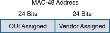
![]() Unicast: A unicast address is associated with a particular device’s NIC or port. It is composed of two sections. The first 24 bits contain the Organizational Unique Identifier (OUI) assigned to an organization. Although this is unique for an organization, the same organization can request several OUIs. For example, Cisco has multiple registered OUIs. The other portion of the MAC address (for example, the remaining 24 bits in the case of MAC-48) can be assigned by the vendor itself.
Unicast: A unicast address is associated with a particular device’s NIC or port. It is composed of two sections. The first 24 bits contain the Organizational Unique Identifier (OUI) assigned to an organization. Although this is unique for an organization, the same organization can request several OUIs. For example, Cisco has multiple registered OUIs. The other portion of the MAC address (for example, the remaining 24 bits in the case of MAC-48) can be assigned by the vendor itself.
Figure 1-11 shows the two portions of a MAC address.
Ethernet Devices and Frame-Forwarding Behavior
So far we have discussed the basic concepts of Ethernet, such as frame formats and addresses. It is now time to see how all this works in practice. We will start with the most basic case and progress toward a more complicated frame forwarding behavior and topology.
LAN Hubs and Bridges
As discussed previously, a collision domain is defined as two or more stations needing to share the same medium. This setup requires some algorithm to avoid two frames being sent at nearly the same time and thus colliding. When a collision occurs, the information is lost. CSMA/CD has been used to resolve the collision problem by allowing an Ethernet station to detect a collision and avoid retransmitting at the same time.
The simplest example of a collision domain is an Ethernet bus where all the stations are connected as shown in Figure 1-12.
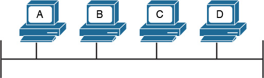
Because the Ethernet signal will degrade across the distance between the stations, the same topology could be obtained by using a central LAN hub where all the stations connect. The role of the LAN hub or repeater was to regenerate the signal uniquely and transmit this signal to all its ports. This topology is typically half-duplex transmission mode and, as in the case of an Ethernet bus, defines a single collision domain.
Figure 1-13 shows how the information sent by Host A is repeated over all the hub’s ports.
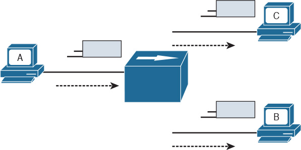
Figure 1-13 A Network Hub Where the Electrical Signal of a Frame Is Regenerated and the Information Sent Out to All the Device Ports
Before transmitting, a station senses the medium (also called carrier) to see if any frame is being transmitted. If the medium is empty, the station can start transmitting. If two stations start at nearly the same time, as is the case in this example, a collision occurs. All stations in the collision domain detect the collision and adopt a backoff algorithm to delay the transmission.
Figure 1-14 shows an example of a collision happening with a hub network. Note that B will also receive a copy of the frame sent from C, and C will receive a copy of the frame sent from B; although, this is not shown in the picture for simplicity.
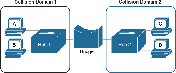
Collision domains are highly inefficient because two stations cannot transmit at the same time. The performance becomes even more impacted as the number of stations connected to the same hubs increases. To partially overcome that situation, networking bridges are used. A bridge is a device that allows the separation of collision domain.
Unlike a LAN hub, which will just regenerate the signal, a LAN bridge typically implements some frame-forwarding decision based on whether or not a frame needs to reach a device on the other side of the bridge.
Figure 1-15 shows an example of a network with hubs and bridges. The bridges partition the network into two collision domains, thus allowing the size of the network to scale.
LAN Switches
In modern networks, half-duplex mode has been replaced by full-duplex mode. Full-duplex mode allows two stations to transmit simultaneously because the transmission and receiver channels are separated. Because of that, in full duplex, CSMA/CD is not used because collisions cannot occur.
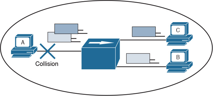
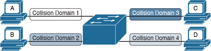
A LAN switch is a device that allows multiple stations to connect in full-duplex mode. This creates a separate collision domain for each of the ports, so collisions cannot happen. For example, Figure 1-16 shows four hosts connected to a switch. Each host has a separate channel to transmit and receive, so each port actually identifies a collision domain. Note that usually in this kind of scenario it does not make sense to refer to a port as collision domain, and it is usually more practical to assume that there is no collision domain—because no collision can occur.
How does a switch forward a frame? Whereas a hub would just replicate the same information on all the ports, a switch tries to do something a bit more intelligent and use the destination MAC address to forward the frame to the right station.
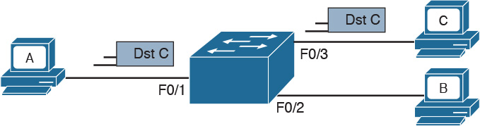
Figure 1-17 shows a simple example of frame forwarding.
How does a switch know to which port to forward a frame? Before this forwarding mechanism can be explained, we need to discuss three concepts:
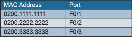
![]() MAC address table: This table holds the link between a MAC address and the physical port of the switch where frames for that MAC address should be forwarded.
MAC address table: This table holds the link between a MAC address and the physical port of the switch where frames for that MAC address should be forwarded.
Figure 1-18 shows an example of a simplified MAC address table.
![]() Dynamic MAC address learning: It is possible to populate the MAC address table manually, but that is probably not the best use of anyone’s time. Dynamic learning is a mechanism that helps with populating the MAC address table. When a switch receives an Ethernet frame on a port, it notes the source MAC address and inserts an entry in the MAC address table, marking that MAC address as reachable from that port.
Dynamic MAC address learning: It is possible to populate the MAC address table manually, but that is probably not the best use of anyone’s time. Dynamic learning is a mechanism that helps with populating the MAC address table. When a switch receives an Ethernet frame on a port, it notes the source MAC address and inserts an entry in the MAC address table, marking that MAC address as reachable from that port.
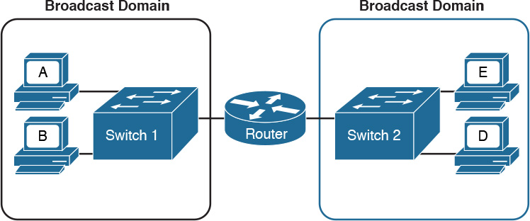
![]() Ethernet Broadcast domain: A broadcast domain is formed by all devices connected to the same LAN switches. Broadcast domains are separated by network layer devices such as routers. An Ethernet broadcast domain is sometimes also called a subnet.
Ethernet Broadcast domain: A broadcast domain is formed by all devices connected to the same LAN switches. Broadcast domains are separated by network layer devices such as routers. An Ethernet broadcast domain is sometimes also called a subnet.
Figure 1-19 shows an example of a network with two broadcast domains separated by a router.
Now that you have been introduced to the concepts of a MAC address table, dynamic MAC address learning, and broadcast domain, we can look at a few examples that explain how the forwarding is done.
The forwarding decision is uniquely done based on the destination MAC address. In this example, Host A with MAC address 0200.1111.1111, connected to switch port F0/1, is sending traffic (Ethernet frames) to Host C with MAC address 0200.3333.3333, connected to port F0/3.
At the beginning, the MAC address table of the switch is empty. When the first frame is received on port F0/1, the switch does two things:
![]() It looks up the MAC address table. Because the table is empty, it forwards the frame to all its ports except the one where the frame was received. This is usually called flooding.
It looks up the MAC address table. Because the table is empty, it forwards the frame to all its ports except the one where the frame was received. This is usually called flooding.
![]() It uses dynamic MAC address learning to update the MAC address table with the information that 0200.1111.1111 is reachable through port F0/1.
It uses dynamic MAC address learning to update the MAC address table with the information that 0200.1111.1111 is reachable through port F0/1.
Figure 1-20 shows the frame flooding and the MAC address table updated with the information about Host A.
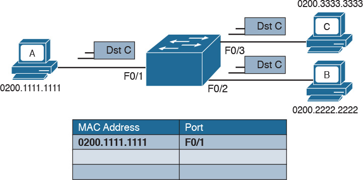
Figure 1-20 Example of a MAC Address Table Being Updated as the Frame Is Received and Forwarded by the Switch
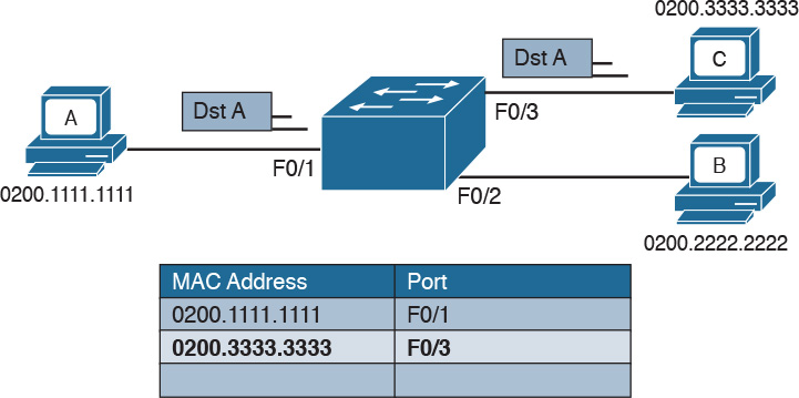
Host B receives a copy of the frame; however, because the destination MAC address is not its own, it discards the frame. Host C receives the frame and may decide to respond. When Host C responds, the switch will look up the MAC address table. This time, it will find an entry for Host A and will just forward the frame on port F0/1 toward Host A. Like in the previous case, it will update the MAC address table to indicate that 0200.3333.3333 (Host C) is reachable through port F0/3, as shown in Figure 1-21.
The flooding mechanism is also used when a frame has a broadcast destination MAC address. In that case, the frame will be forwarded to all ports in the Ethernet broadcast domain. In a more complex topology, switches may be connected to each other, sometimes with multiple ports to ensure redundancy; however, the basic forwarding principles do not change. All MAC addresses that are reachable via other switches will be marked in the MAC address table as reachable via the port where the switches are connected.
Figure 1-22 shows an example of Host A connected to port F0/1 of Switch 1 and sending traffic to Host E, connected to F0/1 of Switch 2. Switch 1 and Switch 2 are connected via port F0/10 on both sides.
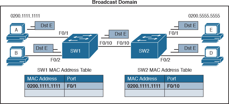
Figure 1-22 Frame Forwarding and MAC Address Table Updates with Multiple Switches. Host A sends a frame for Host E.
When Host A sends the first frame, Switch 1 will flood it on all ports, including on port F0/10 toward Switch 2. Switch 2 will also flood on all its ports because it does not know where Host E is located. Both Switch 1 and Switch 2 will use dynamic learning to update their own MAC address tables. Switch 1 will mark Host A as reachable via F0/1, while Switch 2 will mark Host A as reachable via F0/10.
If Host E responds to Host A, the same steps will be repeated, as shown in Figure 1-23.
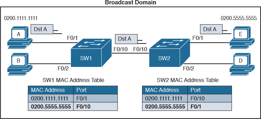
Figure 1-23 Frame Forwarding and MAC Address Table Updates with Multiple Switches. Host E replies to a frame sent by Host A.
Link Layer Loop and Spanning Tree Protocols
Let’s now consider another example, shown in Figure 1-24, where three switches (SW1, SW2, and SW3) are interconnected.
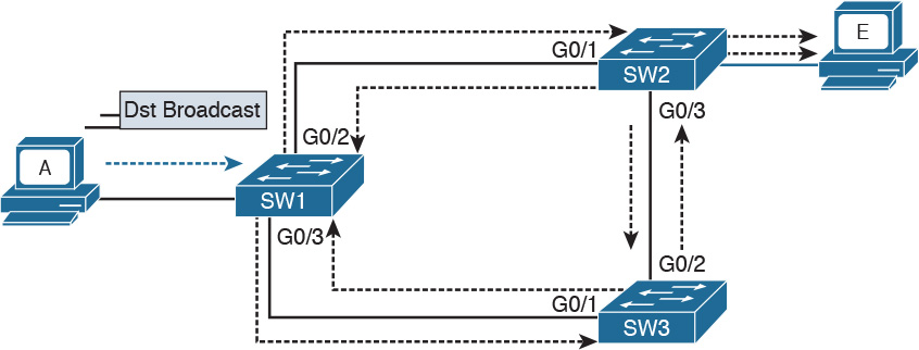
Assume that Host A, connected to SW1, sends a broadcast frame. SW1 will forward the frame to SW2 and SW3 on ports G0/2 and G0/3. SW2 will receive the frame and forward it to SW3 and Host E. SW3 will do the same and forward the frame to SW2. SW3 will again receive the frame from SW2 and will forward it to SW1, and so on.
As you can see, the frame will loop indefinitely within the LAN, thus causing degradation of the network performance due to the useless forwarding of frames. This is called a broadcast storm. Other types of loops can happen—for example, if Host A would have sent a frame to a host that never replies (hence, no switches know where the host is). In general, link layer (or Layer 2) loops can happen every time there is a redundant link within the Layer 2 topology.
The second undesirable effect of Layer 2 loops is MAC table instability. SW1 in the preceding example will keep (incorrectly) updating the MAC address table, marking Host A on port G0/2 and G0/3 as it receives the looping frames with the source address of Host A on these two ports. So, whenever SW1 receives frames for Host A, it will incorrectly send them to the wrong port, making the problem worse.
The third effect of a Layer 2 loop is that a host (for example, Host E) will keep receiving a copy of the same frame that’s circulating within the network. This can confuse the host and may result in higher-layer protocol failure.
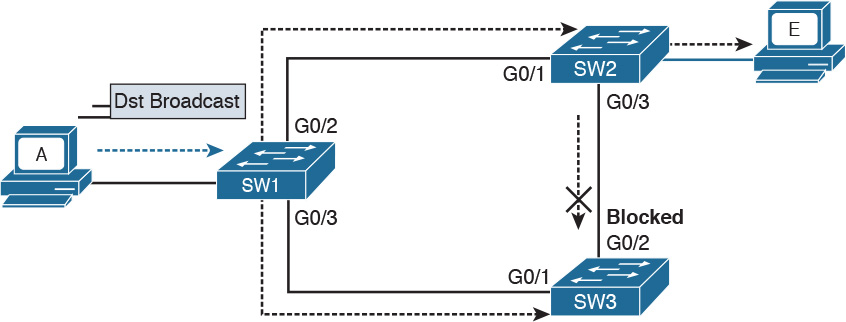
Spanning Tree Protocols (STPs) are used to avoid Layer 2 loops. This section describes the fundamental concepts of STPs. Over the years, the concept has been enhanced to improve performance and to take into consideration the evolution of network complexity. In its basic function, the STP creates a logical Layer 2 topology that is loop free. This is done by allowing traffic on certain ports and blocking traffic on others. If the topology changes (for example, if a link fails), STP will recalculate the new logical topology (it is said to “reconverge”) and unblock certain ports to adapt to the new topology.
Figure 1-25 shows STP applied to the previous example. Port G0/2 on SW3 is marked as blocked, and it will not forward traffic. This avoids frames looping. If the link between SW1 and SW3 goes down, STP will unblock the link between SW3 and SW2 to allow traffic to pass and provide redundancy.
STP uses a spanning tree algorithm (STA) to create a tree-like, loop-free logical topology. To understand how a basic STP works, we need to explore a few concepts:
![]() Bridge ID (BID): An 8-byte ID that is independently calculated on each switch. The first 2 bytes of the BID contain the priority, while the remaining 6 bytes includes the MAC address of the switch (of one of its ports).
Bridge ID (BID): An 8-byte ID that is independently calculated on each switch. The first 2 bytes of the BID contain the priority, while the remaining 6 bytes includes the MAC address of the switch (of one of its ports).
![]() Bridge PDU (BPDU): Represents the STP protocol messages. The BPDU is sent to a multicast MAC address. The address may depend on the specific STP protocol in use.
Bridge PDU (BPDU): Represents the STP protocol messages. The BPDU is sent to a multicast MAC address. The address may depend on the specific STP protocol in use.
![]() Root switch: Represents the root of the spanning tree. The spanning tree root is identified through a process called root election. The root switch BID is called the root BID.
Root switch: Represents the root of the spanning tree. The spanning tree root is identified through a process called root election. The root switch BID is called the root BID.
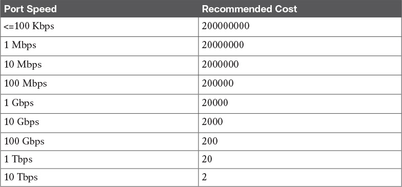
![]() Port cost: A numerical value associated to each spanning tree port. Usually this value depends on the speed of the port. The higher the speed, the lower the cost. Table 1-6 reports the recommended values from IEEE (in IEEE 802.1Q-2014).
Port cost: A numerical value associated to each spanning tree port. Usually this value depends on the speed of the port. The higher the speed, the lower the cost. Table 1-6 reports the recommended values from IEEE (in IEEE 802.1Q-2014).
![]() Root cost: Represents the cost to reach the root switch. The root cost is given by summing all the costs of the ports on the shortest path to the root switch. The root cost value of the root switch is 0.
Root cost: Represents the cost to reach the root switch. The root cost is given by summing all the costs of the ports on the shortest path to the root switch. The root cost value of the root switch is 0.
At initialization, an STP root switch needs to be identified. The root switch will be the switch with the lower BID. The BID priority field is used first to determine the lower BID; if two switches have the same priority, then the MAC address is used to determine the root.
The process to identify the switch with the lower BID is called root election. At the beginning, each switch tries to become the root and sends out a Hello BPDU to announce its presence in the network to the rest of the switches. The initial Hello BPDU includes its own switch BID as the root BID in the BPDU field.
When a switch receives a Hello BPDU with a better root BID (lower BID), it will stop sending its own Hello BPDU and will forward the Hello BPDU generated from the root switch. It will also update the root cost and add the cost of the port where the BPDU was received. The process continues until the root election is over and a root switch is identified. At this point, all switches on the network know which switch is the root and what the root cost is to that switch. Figure 1-26 shows an example of root election in our sample topology.
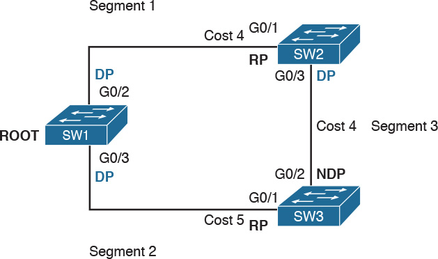
SW1 will send a BPDU to SW2 and SW3. When SW2 receives the BPDU from SW1, it will see that the BID for SW1 is lower than its own BID, so it will update the Root BID entry to include the BID of SW1. SW2 will then forward the BPDU to SW3 with a root cost of 4.
SW3 has also received the BPDU from SW1 and already updated the Root BID entry with SW1’s BID because it is lower than its own BID. It will then forward the BPDU to SW2 with a root cost of 5. At the end, SW1 becomes the root within this topology.
As stated at the beginning of this section, the spanning tree is created by blocking a certain port. Once the root switch is elected, the tree can start to be built. At this point, we need to discuss the concepts of port role and port state:
![]() Port role: Depending on the STP-specific protocols, there are a few names and roles for ports; however, three main roles are important for understanding how STP works. Once that is clear, the nuances of the various STP protocols can be easily understood.
Port role: Depending on the STP-specific protocols, there are a few names and roles for ports; however, three main roles are important for understanding how STP works. Once that is clear, the nuances of the various STP protocols can be easily understood.
![]() Root port (RP) is the port that offers the lowest path cost (root cost) to the root on non-root switches.
Root port (RP) is the port that offers the lowest path cost (root cost) to the root on non-root switches.
![]() Designated port (DP) is the port that offers the lowest path to the root for a given LAN segment. For example, if a switch has a host attached to a port, that port becomes a DP because it’s the closest port to the root for that LAN segment. The switch is told to be the designated switch for that LAN segment. All ports on a root switch are DP.
Designated port (DP) is the port that offers the lowest path to the root for a given LAN segment. For example, if a switch has a host attached to a port, that port becomes a DP because it’s the closest port to the root for that LAN segment. The switch is told to be the designated switch for that LAN segment. All ports on a root switch are DP.
![]() Non-designated ports are all the other ports that are not either the RP or DP. Depending on the specific STP standards, they can assume various names, and the standard can define additional port categories.
Non-designated ports are all the other ports that are not either the RP or DP. Depending on the specific STP standards, they can assume various names, and the standard can define additional port categories.
Let’s look again at our topology, but in a bit different way. Referring to Figure 1-26, we can identify three segments. On the root switch, SW1, all ports are DPs because they offer the shortest path to the root for Segments 1 and 2. What is the DP for Segment 3? Port G0/3 on SW2 will become the DP because its cost to the root is 4, whereas Port G0/2 on SW3 would have a cost of 5.
The RP identification is a bit easier. For each port on a non-root switch, we select the port with the lower path to the root. In this case, G0/1 on SW2 and G0/1 on SW3 become the RP. All remaining ports will be non-designated ports.
![]() Port state: The port state is related to the specific action a port can take while in that state. As in the port role definition, the name of the state depends on the STP protocol being used. Here are some common examples of port states:
Port state: The port state is related to the specific action a port can take while in that state. As in the port role definition, the name of the state depends on the STP protocol being used. Here are some common examples of port states:
![]() Blocking: In this state, a port blocks all frames received except Layer 2 management frames (for example, BPDU).
Blocking: In this state, a port blocks all frames received except Layer 2 management frames (for example, BPDU).
![]() Listening: A port transitions to this state from the blocking state when the STP determines that the port needs to participate in the forwarding. At this stage, however, the port is not fully functional. It can process BPDU and respond to Layer 2 management messages, but it does not accept frames.
Listening: A port transitions to this state from the blocking state when the STP determines that the port needs to participate in the forwarding. At this stage, however, the port is not fully functional. It can process BPDU and respond to Layer 2 management messages, but it does not accept frames.
![]() Learning: The port transitions to learning after the listening phase. In this phase, the port still does not forward frames; however, it learns the MAC addresses via dynamic learning and fills in the MAC address table.
Learning: The port transitions to learning after the listening phase. In this phase, the port still does not forward frames; however, it learns the MAC addresses via dynamic learning and fills in the MAC address table.
![]() Forwarding: In this state, the port is fully operational and receives and forwards frames.
Forwarding: In this state, the port is fully operational and receives and forwards frames.
![]() Disabled: A port in disable state does not forward and receive frames and does not participate in the STP process, so it does not process BPDU.
Disabled: A port in disable state does not forward and receive frames and does not participate in the STP process, so it does not process BPDU.
When the STP protocol has converged, which means the RPs and DPs are identified, each port transitions to a terminal state. Every RP and DP will be in the forwarding state, while all the other ports will be in the blocking state. Figure 1-27 shows the terminal state of the ports in our topology.

STP provides a critical function within communication networks, so a wrong design or implementation of the Spanning Tree Protocol (for example, an incorrect selection of the root switch) could lead to poor performance or even catastrophic failure in some cases.
Through the years, Spanning Tree Protocols have seen several updates and new standards have emerged. The most common versions of Spanning Tree Protocols in use today are Rapid STP, Per-VLAN STP+ (PVSTP+), and Multiple Spanning Tree (MST).
Virtual LAN (VLAN) and VLAN Trunking
So far, we have assumed that everything happens within a single LAN. In simple terms, a LAN can be identified as a part of the network within a single broadcast domain. LANs (and broadcast domains) are separated by Layer 3 devices such as routers.
As the network grows and becomes more complex, operating within a single broadcast domain degrades the network performance and adds complexity to management protocols, such as to the STP.
The concept of a virtual LAN (VLAN) has been introduced to overcome the issues created by a very large single LAN. A VLAN can exist within a switch, and each switch port can be assigned to a specific VLAN.
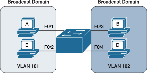
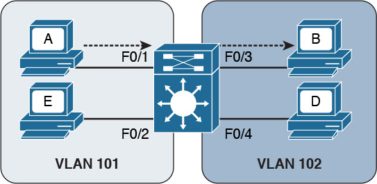
Figure 1-28 shows four hosts connected to the same switch. Host A and Host E are assigned to VLAN 101 whereas Host B and Host D are assigned to VLAN 102. The switch treats a host in one VLAN as being in a single broadcast domain. A packet from one VLAN cannot be forwarded to a different VLAN at Layer 2. As such, a VLAN provides Layer 2 network separation.
Here are some common benefits of using a VLAN:
![]() Reduces the number of devices receiving the broadcast frame and the related overhead
Reduces the number of devices receiving the broadcast frame and the related overhead
![]() Creates Layer 2 network separation
Creates Layer 2 network separation
![]() Reduces management protocols’ load and complexity
Reduces management protocols’ load and complexity
![]() Segments troubleshooting and failure areas, as failure in one VLAN will not be propagated to the rest of the network
Segments troubleshooting and failure areas, as failure in one VLAN will not be propagated to the rest of the network
How does frame forwarding work in VLANs? The same process we described for a single LAN applies for each VLAN. The switch knows which port is linked to which VLAN and will forward the frame accordingly. In the case of multiple switches, the VLAN concept can still work. Figure 1-29 shows the VLAN concept across two switches.
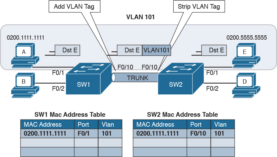
In this case, Host A and Host E, although attached to two different switches, can still be configured within the same VLAN (for example, VLAN 101). The link between SW1 and SW2 is called a trunk, and it is a special link because it can transport frames belonging to several VLANs.
VLAN tagging is used to enable the forwarding between Host A and Host E within the same VLAN as well as across multiple switches. Referring to Figure 1-29, when Host A sends a frame to Host E, SW1 does not know where Host E is, so it will forward the frame to all ports in VLAN 101, including the trunk port to SW2.
As you can see, SW1 will not forward the frame to Host B because it is in a different VLAN. SW1, before sending the frame on the trunk link to SW2, will add a VLAN tag to the frame that carries the VLAN ID, VLAN 101. This tells SW2 that this frame should be forwarded to ports in VLAN 101 only.
SW2 receives the frame over the trunk link, strips the VLAN tagging, and forwards the frame to all its ports in VLAN 101 (in this case, only to F0/1). If Host E responds, the same process applies. SW2 will only send the packets over the trunk link (because SW2 now knows how to reach Host A) and will tag the packet with VLAN 101.
The VLAN information is added to the Ethernet frame. The way that it’s done depends on the protocol used for trunking. The most known and used trunking protocol nowadays is defined in IEEE 802.1Q (dot1q). Another protocol is Inter-Switch Link (ISL), which is a Cisco proprietary protocol that was used in the past.
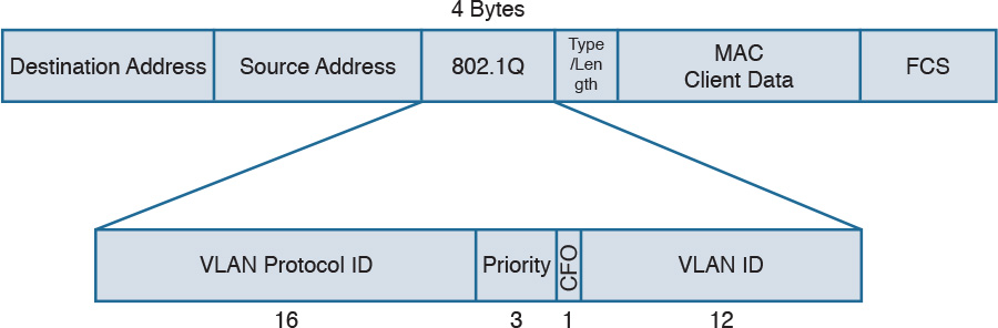
In IEEE 802.1Q, the VLAN tagging is obtained by adding an IEEE 802.1Q tag between the source MAC address and the Type field in the Ethernet frame.
Figure 1-30 shows an example of an IEEE 802.1Q tag. The tag includes the VLAN ID.
IEEE 802.1Q introduces the concept of a native VLAN. The difference between a native and non-native VLAN is that a native VLAN goes without tag over the trunk link. When the trunk is configured for IEEE 802.1Q, if a switch receives a frame without a tag over a trunk link, it will interpret it as belonging to the native VLAN and forward accordingly.
Cisco VLAN Trunking Protocol
Cisco VLAN Trunking Protocol (VTP) is a Cisco proprietary protocol used to manage VLAN distribution across switches. VTP should not be confused with protocols that actually handle the tagging of frames with VLAN information when being sent over a trunk link. VTP is used to distribute information about existing VLANs to all switches in a VTP domain so that VLANs do not have to be manually configured, thus reducing the burden of the administrator.
For example, when a new VLAN is created on one switch, the same VLAN may need to be created on all switches to enable VLAN trunking and consistent use of VLAN IDs. VTP facilitates the process by sending automatic advertisements about the state of VLAN databases across the VTP domain. Switches that receive advertisements will maintain the VLAN database, synchronized based on the information found in the VTP message.
VTP relies on protocols such as 802.1Q to transmit information. VTP defines three modes of operation:
![]() Server mode: In VTP server mode, the administrator can configure or remove a VLAN. VTP will take care of distributing the information to other switches in the VTP domain.
Server mode: In VTP server mode, the administrator can configure or remove a VLAN. VTP will take care of distributing the information to other switches in the VTP domain.
![]() Client mode: In VTP client mode, a switch receives updates about a VLAN and advertises the VLAN configured already; however, a VLAN cannot be added or removed.
Client mode: In VTP client mode, a switch receives updates about a VLAN and advertises the VLAN configured already; however, a VLAN cannot be added or removed.
![]() Transparent mode: In transparent mode, the switch does not participate in VTP, so it does not perform a VLAN database update and does not generate VTP advertisement; however, it forwards VTP advertisements from other switches.
Transparent mode: In transparent mode, the switch does not participate in VTP, so it does not perform a VLAN database update and does not generate VTP advertisement; however, it forwards VTP advertisements from other switches.
Inter-VLAN Traffic and Multilayer Switches
As described in the previous section, VLANs provide a convenient way to separate broadcast domains. This means, however, that a Layer 3 device is needed to forward traffic between two VLANs even if they are on the same switch. We have defined switches as Layer 2 devices, so a switch by itself would not be able to forward traffic from one VLAN to the other, even if the source and destination host reside physically on the same switch.
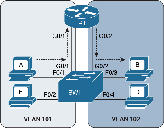
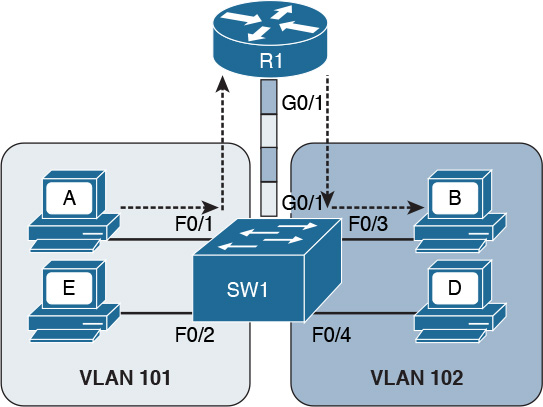
Figure 1-31 shows an example of inter-VLAN traffic. Host A in VLAN 101 is sending traffic to Host B in VLAN 102. Both hosts are connected to SW1. Because SW1 is a switch operating at Layer 2, a Layer 3 device (for example, a router, R1) is needed to forward the traffic. In the figure, the router uses two different interfaces connected to the switch, where G0/1 is in VLAN 101 and G0/2 is in VLAN 102.
Alternatively, R1 could have been configured with only one interface on the switch with trunking enabled. This alternative is sometimes defined as router on a stick (ROAS), as illustrated in Figure 1-32.
In both of the preceding examples, there is a waste of resources. For example, a packet needs to travel to the first router in the path, to then come back again to the same switch creating additional load on the links. Additionally, there is a loss in performance due to the encapsulation and upper-layer processing of the frame.
The solution is to integrate Layer 3 function within a classic Layer 2 switch. This type of switch is called a Layer 3 switch or sometimes a multilayer switch. Figure 1-33 shows an example of inter-VLAN flow with a multilayer switch.
Wireless LAN Fundamentals and Technologies
Together with Ethernet, which is defined as wired access to a LAN, wireless LAN (WLAN) is one of the most used technologies for LAN access. This book covers the basics of WLAN fundamentals and technologies. Interested readers can refer to the CCNA Wireless 200-355 Official Cert Guide book for additional information.
Wireless LAN is defined within the IEEE 802.11 standards. While in some aspects WLANs resemble classic Ethernet technology, there are several significant differences.
The first and most notable difference is the medium. Here are several other characteristics that distinguish a wireless medium from a wire medium:
![]() There is no defined boundary.
There is no defined boundary.
![]() It is more prone to interference by other signals on the same medium.
It is more prone to interference by other signals on the same medium.
![]() It is less reliable.
It is less reliable.
![]() The signal can propagate in asymmetric ways (for example, due to reflection).
The signal can propagate in asymmetric ways (for example, due to reflection).
The way stations access the medium is also different. In the previous section, you learned that Ethernet defines two operational modes: half duplex, where the stations can transmit one at time, and full-duplex, where stations can transmit simultaneously. In WLANs, network stations can only use half-duplex mode because they are not able to transmit and receive at the same time due to the limitation of the medium.
This means that two stations need to implement a way to detect if the medium (in this case, the radio frequency channel) is being used to avoid transmitting at the same time. This functionality is provided by a Carrier Sense Media Access with Collision Avoidance (CSMA/CA). Note that this is different from the CSMA/CD used in Ethernet. The main difference is in how a collision is handled. Wired devices can detect collisions over the medium, whereas wireless devices cannot.
Like we have seen for Ethernet, a wireless station senses the medium to determine whether is it possible to transmit. However, the way this is done is different for wired devices. In a wired technology, the device can sense an electrical signal on the wire and determine whether someone else is transmitting. This cannot happen in the case of wireless devices. There are mainly two methods for carrier sense:
![]() Physical carrier sense: When the station is not transmitting, it can sense the channel for the presence of other frames. This is sometimes referred to as Clear Channel Assessment (CCA).
Physical carrier sense: When the station is not transmitting, it can sense the channel for the presence of other frames. This is sometimes referred to as Clear Channel Assessment (CCA).
![]() Virtual carrier sense: Stations when transmitting a frame include an estimated time for the transmission of the frame in the frame header. This value can be used to estimate how long the channel will be busy.
Virtual carrier sense: Stations when transmitting a frame include an estimated time for the transmission of the frame in the frame header. This value can be used to estimate how long the channel will be busy.
Collision detection is not possible for similar reasons. Wireless clients thus need to avoid collisions. To do that, they use a mechanism called Collision Avoidance. The mechanism works by using backoff timers. Each station waits a backoff period before transmitting. In addition to the backoff period, a station may need to wait for an additional time, called interframe space, which is used to reduce the likelihood of a collision and to allow an extra cushion of time between two frames.
802.11 defines several interframe space timers. The standard interframe timer is called Distributed Interframe Space (DIFS).
The basic process of transmitting frames includes three steps:
Step 1. Sense the channel to see whether it is busy.
Step 2. Select a delay based on the backoff timer. If, in the meantime, the channel gets busy, the backoff timer is stopped. When the channel is clear again, the backoff timer is restarted.
Step 3. Wait for an additional DIFS time.
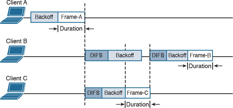
Figure 1-34 illustrates the process of transmitting frames in a WLAN. Client A is ready to transmit, it senses the medium, selects a backoff time, and then transmits. The duration of the frame is included in the frame header. Client B and Client C wait until the frame from Client A has been transmitted plus the DIFS, and then start the backoff timer. Client C’s backoff timer expires before Client B’s, so Client C transmits before Client B. Client B finds the channel busy, so it stops the backoff timer. Client B waits for the new transmission time, the DIFS period and the remaining backoff timer, and then it transmits.
One particularity of WLANs compared to wired networks is that a WLAN requires the other party to send an acknowledgement so that the sender knows the frame has been received.
802.11 Architecture and Basic Concepts
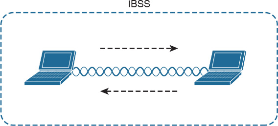
Unlike wired connections, where a station needs a physical connection to be able to transmit, the wireless medium is open, so any station can start transmitting. The IEEE 802.11 standards define the concept of Basic Service Set (BSS), which identifies a set of devices that share some common parameters and can communicate through a wireless connection. The most basic type of BSS is called Independent BSS (IBSS), and it is formed by two or more wireless stations communicating directly. IBSS is sometimes called ad-hoc wireless network.
Figure 1-35 shows an example of IBSS.
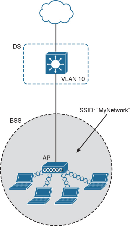
Another type of BSS is called infrastructure BSS. The core of an infrastructure BSS is a wireless access point, or simply an access point (AP). Each station will associate to the AP, and each frame is sent to the AP, which will then forward it to the receiving station. The access point advertises a Service Set Identifier (SSID), which is used by each station to recognize a particular network.
To communicate with other stations that are not in the same BSS (for example, a server station in the organization’s data center), access points can be connected in uplink with the rest of the organization’s network (for example, with a wired connection). The uplink wired network is called a Distribution System (DS). The AP creates a boundary point between the BSS and the DS.
Figure 1-36 shows an example of infrastructure BSS with four wireless stations and an access point connected upstream with a DS.
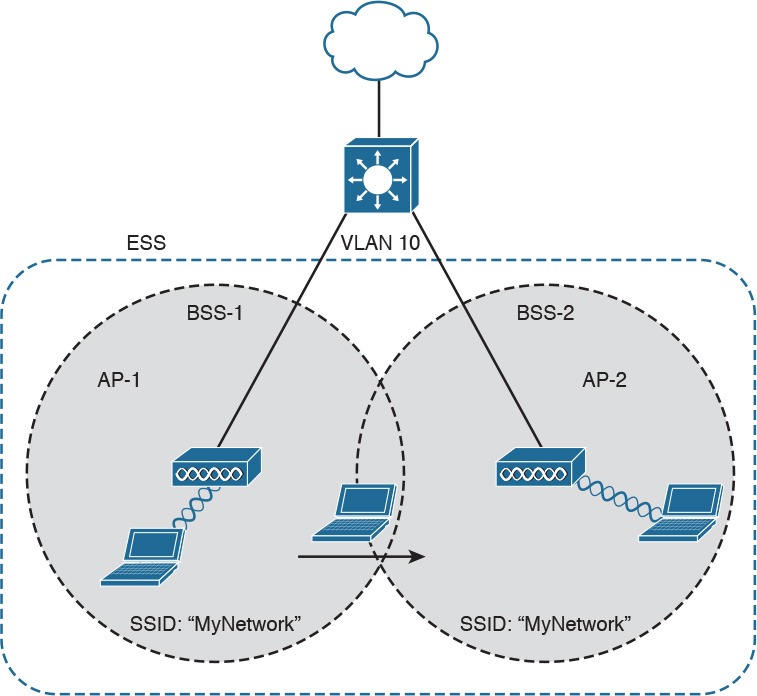
An access point has limited spatial coverage due to the wireless signal degradation. To extend the wireless coverage of a specific network (that is, a network identified by a single SSID), multiple BSSs can be linked together to form an Extended Service Set (ESS). A client can move from one AP to the other in a seamless way. The method to release a client from one AP and associate to the other AP is called roaming.
Figure 1-37 shows an example of an ESS with two APs connected to a DS and a user roaming between two BSSs.
802.11 Frame
An 802.11 frame is a bit different from the Ethernet frame, although there are some commonalities. Figure 1-38 shows an example of 802.11 frame.
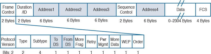
The 802.11 frame includes the following elements:
![]() Frame control: Includes some additional sub-elements, as indicated in Figure 1-37. It provides information on the frame type and whether this frame is directed toward the DS or is coming from the DS toward the wireless network.
Frame control: Includes some additional sub-elements, as indicated in Figure 1-37. It provides information on the frame type and whether this frame is directed toward the DS or is coming from the DS toward the wireless network.
![]() Duration field: Can have different meanings depending on the frame type. However, one common value is the expected time the frame will be traveling on the channel for the Virtual Carrier Sense functionality.
Duration field: Can have different meanings depending on the frame type. However, one common value is the expected time the frame will be traveling on the channel for the Virtual Carrier Sense functionality.
![]() Address fields: Contain addresses in 802 MAC format (for example, MAC-48). The following are the typical addresses included:
Address fields: Contain addresses in 802 MAC format (for example, MAC-48). The following are the typical addresses included:
![]() Transmitter address (TA) is the MAC address of the transmitter of the frame (for example, a wireless client).
Transmitter address (TA) is the MAC address of the transmitter of the frame (for example, a wireless client).
![]() Receiver address (RA) is the MAC address of the receiver of the frame (for example, the AP).
Receiver address (RA) is the MAC address of the receiver of the frame (for example, the AP).
![]() Source address (SA) is the MAC address of the source of the frame, if it is different from the TA. For example, if a frame is coming from the DS toward a wireless station, the SA would be the original Ethernet source address whereas the TA would be the AP.
Source address (SA) is the MAC address of the source of the frame, if it is different from the TA. For example, if a frame is coming from the DS toward a wireless station, the SA would be the original Ethernet source address whereas the TA would be the AP.
![]() Destination address (DA) is the MAC address of the final destination if different from the RA (for example, for a frame destined to the DS).
Destination address (DA) is the MAC address of the final destination if different from the RA (for example, for a frame destined to the DS).
![]() Sequence Control field: This is used for sequence and fragmentation numbering.
Sequence Control field: This is used for sequence and fragmentation numbering.
![]() Frame body: Includes the upper-layer PDU, as in the case of Ethernet.
Frame body: Includes the upper-layer PDU, as in the case of Ethernet.
![]() Frame Check Sequence (FCS) field: Used by the receiving device to detect an error in transmission.
Frame Check Sequence (FCS) field: Used by the receiving device to detect an error in transmission.
WLAN Access Point Types and Management
In the previous sections you learned about the wireless access point (AP). The main functionality of an AP is to bridge frames from the wireless interface to the wired interfaces so that a wireless station can communicate with the rest of the wired network. This means, for example, extracting the payload of an 802.11 frame and re-encapsulating it in an Ethernet frame.
The AP provides additional functionalities that are as important for the correct functionality of a wireless network. For example, an AP needs to manage the association or the roaming of wireless stations, implement authentication and security features, manage the radio frequency (RF), and so on.
The functionality provided by an access point can be classified in two categories:
![]() Real-time functions include all the functionality to actually transmit and receive frames, or to encrypt the information over the channel.
Real-time functions include all the functionality to actually transmit and receive frames, or to encrypt the information over the channel.
![]() Management functions include functions such as RF management, security management, QoS, and so on.
Management functions include functions such as RF management, security management, QoS, and so on.
The access points also can be categorized based on the type of functionality provided:
![]() Autonomous APs are access points that implement both real-time and management functions. These are autonomous and thus work in a standalone mode. Each AP needs to be configured singularly.
Autonomous APs are access points that implement both real-time and management functions. These are autonomous and thus work in a standalone mode. Each AP needs to be configured singularly.
![]() Lightweight APs (LAPs) only implement the real-time functions and work together with a management device called a wireless LAN controller (WLC), which provides the management functions. The communication between LAPs and the WLC is done using the Control and Provision of Wireless Access Point (CAPWAP).
Lightweight APs (LAPs) only implement the real-time functions and work together with a management device called a wireless LAN controller (WLC), which provides the management functions. The communication between LAPs and the WLC is done using the Control and Provision of Wireless Access Point (CAPWAP).
Figure 1-39 shows the difference between the two types of APs.

Depending on the type of AP, the network architecture and packet flow may change. In a network using autonomous AP, the packet flow is similar to a network with a switch, as seen in previous sections. Each wireless client will be associated to a VLAN, and the AP will be configured with a trunk on its DS interface. The AP can participate in STP and will behave much like a switch.
Autonomous APs can be managed singularly or through centralized management software. For example, Cisco Prime Infrastructure can be used to manage several autonomous access points. This type of architecture is called autonomous architecture.
Another option is to use autonomous access points that are managed from the cloud. This is called cloud-based architecture. An example of such a deployment is the Cisco Meraki cloud-based wireless network architecture.
A third option is to use LAPs and WLC. This type of deployment is called split MAC due to the splitting of functionalities between the LAPs and the WLC. The CAPWAP protocol is used for communication between the LAPs and the WLC. CAPWAP is a tunneling protocol described in RFC 5415. It is used to tunnel 802.11 frames from a LAP to the WLC for additional forwarding. The encapsulation is needed because the WLC can reside anywhere in the DS (for example, in a different VLAN than the LAP). CAPWAP encapsulates the 802.11 frame in an IP packet that can be used to reach the WLC regardless of its logical position. CAPWAP uses UDP to provide end-to-end connectivity between the LAP and WLC, and it uses DTLS to protect the tunnels.
CAPWAP consists of two logical tunnels:
![]() CAPWAP control messages, which transport management frames
CAPWAP control messages, which transport management frames
![]() CAPWAP data, which transports the actual data to and from the LAP
CAPWAP data, which transports the actual data to and from the LAP
When a LAP is added to the network, it establishes a tunnel to the WLC. After that, the WLC can push configuration and other management information.
In a split-MAC deployment, when a wireless station sends information, the AP will encapsulate the information using the CAPWAP specification and send it to the WLC. For example, in the case of a WLAN, it will use the CAPWAP protocol binding for 802.11 described in RFC 5416, which also specifies how the 802.11 frame should be encapsulated in a CAPWAP tunnel.
The WLC will then decapsulate the information and send it to the correct recipient. When the recipient responds, the information will flow in the reverse direction—first to the WLC and then through the CAPWAP data tunnel to the AP, which will finally forward the information to the wireless station.
There are two types of split-MAC architectures:
![]() Centralized architecture: This architecture places the WLC in a central location (for example, closer to the core) so that the number of LAPs covered is maximized. One advantage of centralized architecture is that roaming between LAPs is simplified because one WLC controls all the LAPs a user is traversing. However, traffic between two wireless stations associated to the same LAP may need to travel through several links in order to reach the WLC and then back to the same LAP. This may reduce the efficiency of the network.
Centralized architecture: This architecture places the WLC in a central location (for example, closer to the core) so that the number of LAPs covered is maximized. One advantage of centralized architecture is that roaming between LAPs is simplified because one WLC controls all the LAPs a user is traversing. However, traffic between two wireless stations associated to the same LAP may need to travel through several links in order to reach the WLC and then back to the same LAP. This may reduce the efficiency of the network.
Figure 1-40 shows an example of a centralized WLC architecture and the frame path for a wireless-station-to-wireless-station transmission.
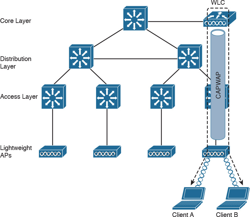
![]() Converged architecture: With this architecture, the WLC is moved closer to the LAPs typically at the access layer. In this case, one WLC is covering fewer LAPs, so various WLCs need to work together in a distributed fashion. In a converged architecture, the WLC may be integrated into the access layer switch, which also provides WLC functionality. This type of architecture increases the performance of wireless-station-to-wireless-station communication, but makes roaming more complicated because the user must travel through several WLCs. Figure 1-41 shows an example of a converged architecture.
Converged architecture: With this architecture, the WLC is moved closer to the LAPs typically at the access layer. In this case, one WLC is covering fewer LAPs, so various WLCs need to work together in a distributed fashion. In a converged architecture, the WLC may be integrated into the access layer switch, which also provides WLC functionality. This type of architecture increases the performance of wireless-station-to-wireless-station communication, but makes roaming more complicated because the user must travel through several WLCs. Figure 1-41 shows an example of a converged architecture.
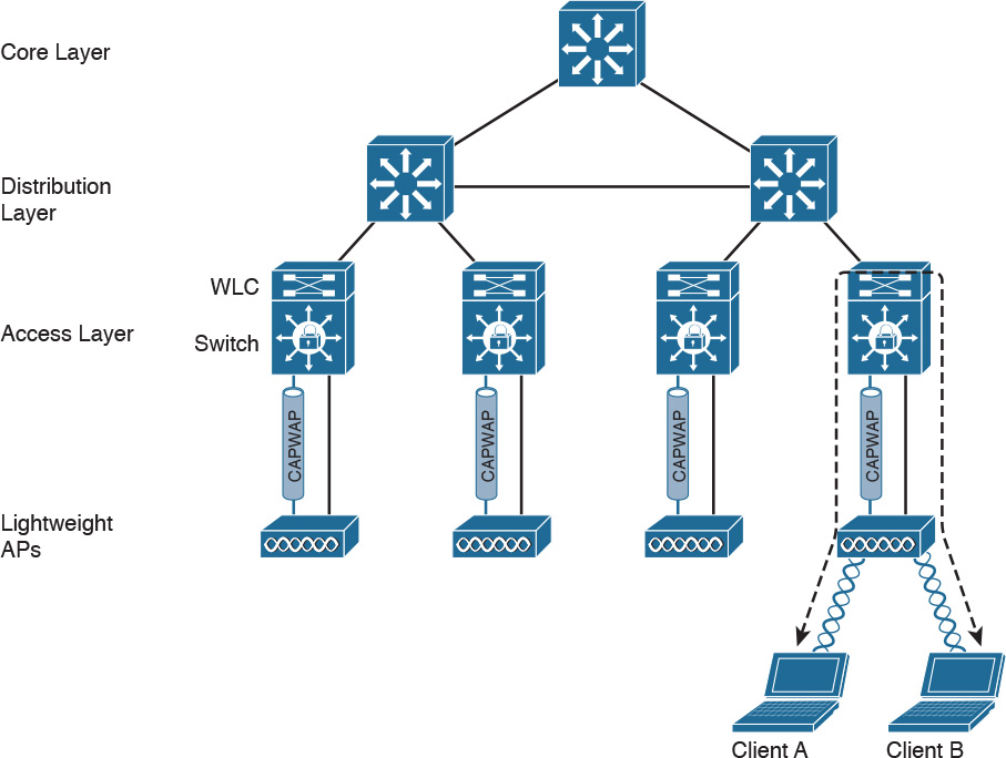
Internet Protocol and Layer 3 Technologies
In previous sections, you learned how information is sent at the link layer, or Layer 2. In this section, we discuss how information is transmitted at Layer 3—that is, how a packet travels through a network, across several broadcast domains, to reach its destination.
Layer 3 protocols are used to enable communication without being concerned about the specific transportation medium or other Layer 2 properties (for example, whether the information needs to be transported on a wired network or using a wireless connection). The most-used Layer 3 protocol is the Internet Protocol (IP). As a security professional, it is fundamental that you master how IP works in communication networks.
IP comes in two different versions: IP version 4 (IPv4) and IP version 6 (IPv6). Although some of the concepts remain the same between the two versions, IPv6 could be seen as a completely different protocol rather than an update of IPv4. In this section, we mainly discuss IPv4. In the next section, we will discuss the fundamentals of IPv6 and highlight the differences between IPv4 and IPv6.
Before digging into more detail, let’s look at the basic transmission of an IP packet, also referred to as Layer 3 forwarding. Figure 1-42 shows a simple topology where Host A is connected to a switch that provides LAN access to the host at Site A. Host B is also connected to an access switch at Site B. In the middle, two routers (R1 and R2) provide connectivity between the two sites.
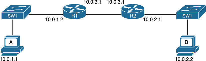
Here are a few concepts you should be familiar with:
![]() An IP address is the means by which a device is identified by the IP protocol. An IP address can be assigned to a host or to a router interface.
An IP address is the means by which a device is identified by the IP protocol. An IP address can be assigned to a host or to a router interface.
In the example in Figure 1-42, Host A is identified by IPv4 address 10.0.1.1, and Host B is identified by IPv4 address 10.0.2.2. IPv4 and IPv6 are different; we will look into the details of IPv4 and IPv6 addresses later in this section.
![]() The routing table or routing database is somewhat similar to the MAC address table discussed in the previous section. The routing table contains two main pieces of information: the destination IP or network and the next-hop IP address, which is the IP address of the next device where the IP packet should be sent.
The routing table or routing database is somewhat similar to the MAC address table discussed in the previous section. The routing table contains two main pieces of information: the destination IP or network and the next-hop IP address, which is the IP address of the next device where the IP packet should be sent.
![]() A default route is a special entry in the routing table that says to forward all packets, regardless of the destination to a specific next hop.
A default route is a special entry in the routing table that says to forward all packets, regardless of the destination to a specific next hop.
![]() Packet routing refers to the action performed by the Layer 3 device to transmit a packet. When a packet reaches one interface of the device, the device will look up the routing table to see where the packet should be sent. If the information is found, the packet is sent to the next-hop device.
Packet routing refers to the action performed by the Layer 3 device to transmit a packet. When a packet reaches one interface of the device, the device will look up the routing table to see where the packet should be sent. If the information is found, the packet is sent to the next-hop device.
![]() The router or IP gateway is a Layer 3 device that performs packet routing. It has two or more interfaces connected to a network segment—either a LAN segment or a WAN segment. Although a router is usually classified as Layer 3, most modern routers implement all layers of the TCP/IP model; however, their main function is to route packets at Layer 3. R1 and R2 in Figure 1-42 are examples of routers.
The router or IP gateway is a Layer 3 device that performs packet routing. It has two or more interfaces connected to a network segment—either a LAN segment or a WAN segment. Although a router is usually classified as Layer 3, most modern routers implement all layers of the TCP/IP model; however, their main function is to route packets at Layer 3. R1 and R2 in Figure 1-42 are examples of routers.
Referring to Figure 1-43, let’s see how Host A can send information to Host B.
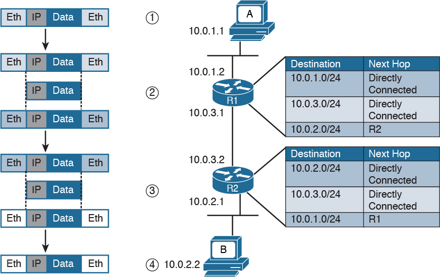
Step 1. Host A will encapsulate the data through the various TCP/IP layers up to the IP layer. The IP layer adds the IP header and sends it down to the link layer to encapsulate it in an Ethernet frame. After that, the frame is sent to R1.
Step 2. R1 strips the Ethernet header and trailer and processes the IP packet header. It sees that this packet has Host B as its destination, so it looks to its routing table to find the next-hop device. In the routing table, Host B can be reached via R2, so R1 re-encapsulates the packet in a new link layer frame (for example, a new Ethernet frame) and sends it to R2.
Step 3. R2 performs the same operation as R1. It strips the link layer information, processes the IP packet header, and looks to its routing table to find Host B. R2 sees that Host B is directly connected—that is, it is in the same broadcast domain as its F0/2 interface—so it encapsulates the packet in an Ethernet frame and sends it directly to Host B.
Step 4. Host B receives the Ethernet frame, strips the information, and reads the IP packet header. Because Host B is the recipient of the packet, it will further process the IP packet to access the payload.
This process is somehow similar for IPv4 and IPv6. We will continue explaining the routing process using IPv4. IPv6 will be discussed a bit down the road.
IPv4 Header
An IP packet is formed by an IP header, which includes information on how to handle the packet from the IP protocol, and by the IP payload, which includes the Layer 4 PDU (for example, the TCP segment). The IP header is between 20 and 60 bytes long, depending on which IP header options are present.
Figure 1-44 shows an example of an IPv4 header.
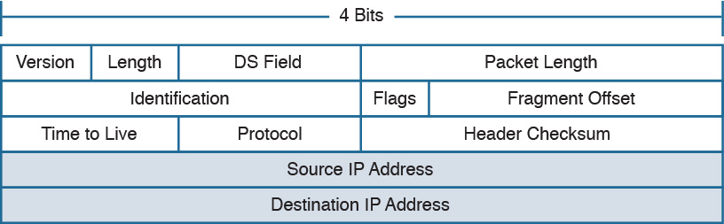
The IP header fields are as follows:
![]() Version: Indicates the IP protocol version (for example, IP version 4).
Version: Indicates the IP protocol version (for example, IP version 4).
![]() Internet Header Length: It indicates the length of the header. A standard header, without options, is 20 bytes in length.
Internet Header Length: It indicates the length of the header. A standard header, without options, is 20 bytes in length.
![]() Notification (Differentiated Services Code Point [DSCP]) and Explicit Congestion (ECN): Includes information about flow prioritization to implement Quality of Service and congestion control.
Notification (Differentiated Services Code Point [DSCP]) and Explicit Congestion (ECN): Includes information about flow prioritization to implement Quality of Service and congestion control.
![]() Total Length: The length of the IP packet, which is the IP header plus the payload. The minimum length is 20 bytes, which is an IP packet that includes the basic IP header only.
Total Length: The length of the IP packet, which is the IP header plus the payload. The minimum length is 20 bytes, which is an IP packet that includes the basic IP header only.
![]() Identification: This field is mainly used when an IP packet needs to be fragmented due to constraint at the Layer 2 protocol. For example, Ethernet can transport, at a maximum, a 1500-byte IP packet.
Identification: This field is mainly used when an IP packet needs to be fragmented due to constraint at the Layer 2 protocol. For example, Ethernet can transport, at a maximum, a 1500-byte IP packet.
![]() Flags and Fragment Offset: Fields to handle IP packet fragmentation.
Flags and Fragment Offset: Fields to handle IP packet fragmentation.
![]() Time to Live (TTL): A field that’s used to prevent IP packets from looping indefinitely. The TTL field is set when the IP packet is created, and each router on the path decrements it by one unit. If the TTL goes to zero, the router discards the packet and sends a message to the sender to tell it that the packet was dropped.
Time to Live (TTL): A field that’s used to prevent IP packets from looping indefinitely. The TTL field is set when the IP packet is created, and each router on the path decrements it by one unit. If the TTL goes to zero, the router discards the packet and sends a message to the sender to tell it that the packet was dropped.
![]() Protocol: Indicates the type of protocol transported within the IP payload. For example, if TCP is transported, the value is 6; if UDP is transported, the value is 17.
Protocol: Indicates the type of protocol transported within the IP payload. For example, if TCP is transported, the value is 6; if UDP is transported, the value is 17.
Table 1-7 lists the common IP protocol codes. The protocol numbers are registered at IANA (http://www.iana.org/assignments/protocol-numbers/protocol-numbers.xhtml).
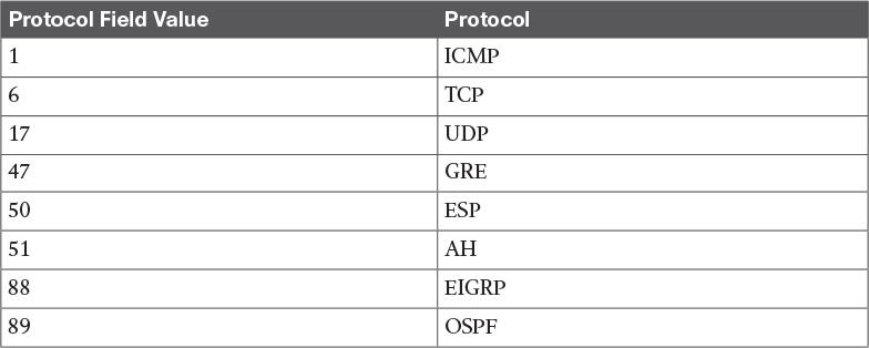
![]() Header Checksum: This is the checksum of the header. Every time a router modifies the header (for example, to reduce the TTL field), the header checksum needs to be recalculated.
Header Checksum: This is the checksum of the header. Every time a router modifies the header (for example, to reduce the TTL field), the header checksum needs to be recalculated.
![]() Source Address: This is the IP address of the sender of the IP packet.
Source Address: This is the IP address of the sender of the IP packet.
![]() Destination Address: This is the IP address of the destination of the IP packet.
Destination Address: This is the IP address of the destination of the IP packet.
IPv4 Fragmentation
IP fragmentation is the process of splitting an IP packet into several fragments to allow the transmission by a Layer 2 protocol. In fact, the maximum length of a payload for a Layer 2 protocol depends on the physical medium used for transmission and on other factors. For example, Ethernet allows a maximum payload for the frame, also called the maximum transmission unit (MTU), of 1500 bytes in its basic frame, as you saw earlier. So what happens if a host sends an IP packet that is larger than that size? The packet needs to be fragmented.
Figure 1-45 shows an example of fragmentation. Host A sends an IP packet that is 2000 bytes, including 20 bytes of IP header. Before being transmitted via Ethernet, the packet needs to be split in two: one fragment will be 1500 bytes, and the other will be 520 bytes (500 bytes are due to the remaining payload, plus 20 bytes for the new IP header, which is added to the second fragment).
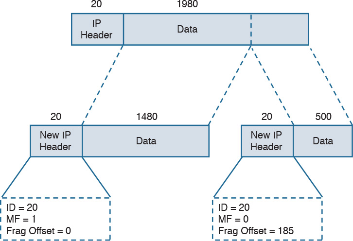
The receiving host reassembles the original packet once all the fragments arrive. Two or more fragments of the same IP packet can be recognized because they will have the same value in the Identification field. The IP flags include a bit called More Fragments (MF), which indicates whether more fragments are expected. The last fragment will have this bit unset to indicate that no more fragments are expected. The Fragment Offset field is used to indicate at which point of the original unfragmented IP packet this fragment should start.
In the example in Figure 1-45, the first packet would have the following fields set:
![]() Identification = 20
Identification = 20
![]() IP Flags MF = 1
IP Flags MF = 1
![]() Fragment Offset = 0
Fragment Offset = 0
The second fragment would have these fields set:
![]() Identification = 20 (which indicates that this is a fragment of the previous packet)
Identification = 20 (which indicates that this is a fragment of the previous packet)
![]() IP Flags MF = 0 (which indicates that this is the last fragment)
IP Flags MF = 0 (which indicates that this is the last fragment)
![]() Fragment Offset = 1480 (to indicate that this fragment should start after 1480 bytes of the original packet)
Fragment Offset = 1480 (to indicate that this fragment should start after 1480 bytes of the original packet)
NOTE
In reality, the fragment offset is expressed in multiples of 8. Therefore, the real value would be 185 (that is, 1480 / 8).
IPv4 Addresses and Addressing Architecture
An IPv4 address is a 32-bit-long number used to identify a device at Layer 3 (for example, a host or a router interface). In human-readable form, an IPv4 address is usually written in dotted decimal notation. The address is split in four parts of 8 bits each, and each part is represented in decimal form.
For example, an IPv4 address of 00000001000000010000000111111110 would be transformed into 00000001. 00000001. 00000001. 11111110, and each octet is transformed to decimal. Therefore, this address is written as 1.1.1.254.
You may be wondering how IP addresses are assigned? For example, who decided that 10.0.1.1 should be the IP address of Host A? Creating the IP address architecture is one of the most delicate tasks when designing an IP-based communication network. This section starts with a description of the basics of IP addressing and then delves into how the concept evolved and how it is commonly performed today.
One of the first architectures, called classful addressing, was based on IPv4 address classes, where the IPv4 address is logically divided into two components: a network part and a host part. The network prefix identifies the network (for example, an organization), while the host number identifies a host within that network.
The IPv4 address range was divided into five classes, as shown in Table 1-8.
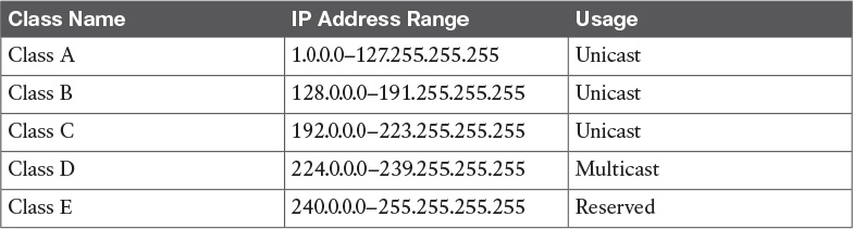
Class A, B, and C IP addresses can be assigned to hosts or interfaces for normal IP unicast usage; Class D IP addresses can be used as multicast addresses; Class E is reserved and cannot be used for IP routing. The network prefix length and host numbering length vary depending on the class.
Class A allots the first 8 bits for the network prefix and the remaining 24 bits for host addresses. This means Class A includes 256 (28) distinct networks, each capable of providing an address to 16,777,216 (224) hosts. For example, address 1.1.1.1 and address 2.2.2.2 would be in two different networks, whereas address 1.1.1.1 and address 1.4.1.1 would be in the same 1.x.x.x Class A network.
Class B allots the first 16 bits for the network prefix and the remaining 16 for host addresses. Class B includes 65,536 (216) distinct networks and 65,536 (216) host addresses within a single network.
Class C allots the first 24 bits for the network prefix and the remaining 8 for host addresses. Class C includes 16,777,216 (28) distinct networks and 256 (28) host addresses within one network.
Figure 1-46 summarizes the network and host portions for each class.
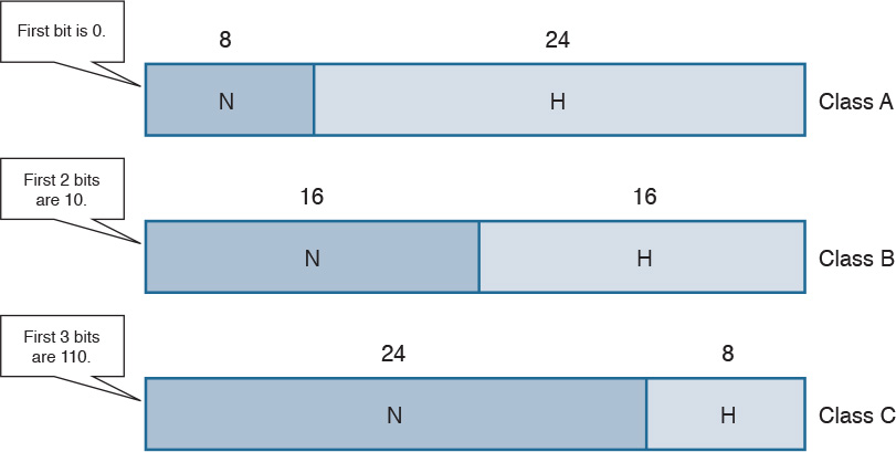
For each network, there are two special addresses that are usually not assigned to a single host:
![]() Network address: An address where the host portion is set to all 0s. This address is used to identify the whole network.
Network address: An address where the host portion is set to all 0s. This address is used to identify the whole network.
![]() Broadcast network address: An address where the host portion is set to all 1s in binary notation, which correspond to 255 in decimal notation.
Broadcast network address: An address where the host portion is set to all 1s in binary notation, which correspond to 255 in decimal notation.
For example, in the network 1.x.x.x, the network address would be 1.0.0.0 and the broadcast address would be 1.255.255.255. To indicate the bits used for the network portion and the bits used for the host portion, each IP address is followed by a network mask.
A network mask is a binary number that has the same length as an IP address: 32 bits. In a network mask, the network portion is indicated with all 1s and the host portion with all 0s. The network mask can also be read in dotted decimal format like an IP address. For example, the network mask for a Class A network would be 11111111000000000000000000000000, or 255.0.0.0.
The network mask sometimes is abbreviated as a backslash character (/) followed by the number of bits of the network portion of the IP address. For example, the same Class A network mask can be written as /8. This is sometime called Classless Interdomain Routing (CIDR) notation. Although it may seem that a network mask is unnecessary because the IP address range already provides the same info (for example, 3.3.3.3 would fall under the Class A addresses range, which would imply a network prefix of 8 bits), network masks are important to the concept of subnets, which we discuss in the next section.
Table 1-9 shows the default network mask for Classes A, B, and C. Classes D and E do not have any predefined mask because they are not used for unicast traffic.
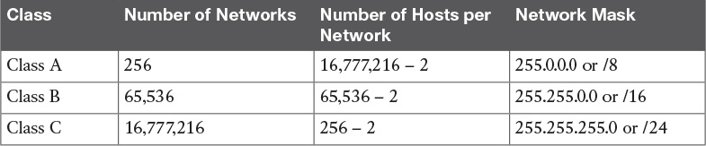
Keep in mind that two hosts are subtracted from the totals in this table because we need to remove the host address reserved for the network address as well as the address reserved for the broadcast network address.
IP Network Subnetting and Classless Interdomain Routing (CIDR)
In the classful addressing model, an organization would need to send a request to an Internet registry authority for a network within one of the classes, depending on the number of hosts needed. However, this method is highly inefficient because organizations receive more addresses than they actually need due to the structure of the classes. For example, an organization that only needs to assign an address to 20 hosts would get a Class C network, thus wasting 234 addresses (that is, 256 – 20 – 2). A more intelligent approach is introduced with Classless Interdomain Routing (CIDR).
CIDR moves away from the concept of class and introduces the concept of a network mask or prefix, as mentioned in the previous section. By using CIDR, the IANA or any local registry can assign to an organization a smaller number of IP addresses instead of having to assign a full class range. With this method, IP addresses can be saved because an organization can request an IP address range that actually fits its requirements, which means other addresses can be allocated to a different organization.
In the previous example, the organization would receive a /27 network mask instead of a full Class C network (/24). In the following pages, we explore how an organization can further partition the received address space to adapt to organizational needs using the concept of subnets.
You were already introduced to the term subnet or network segment when we discussed Layer 2 technologies. A subnet can be identified with a broadcast domain. In Figure 1-47, we can identify three subnets, each representing a separate broadcast domain. Each subnet includes a number of IP addresses that are assigned to the hosts and interfaces within that subnet. In this example, Subnet 1 would need a minimum of three IP addresses (Host A, Host B, and the R1 interface), and Subnet 2 at least two IP addresses (one for each router interface). Subnet 3 also would need at least two IP addresses (one for Host C and one for the R2 interface). Remember than on each subnet, we also need to reserve one address for the network ID and one for the broadcast network address.
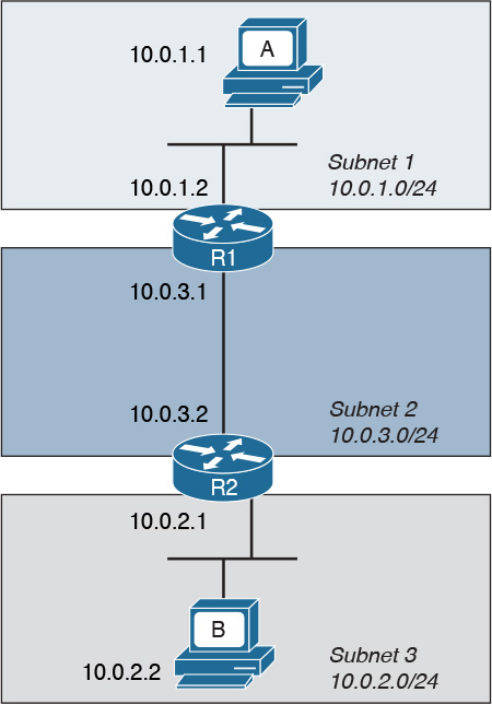
When subnets are used, an IP address is logically split into three parts: the network prefix, the subnet ID, and the host portion, as shown in Figure 1-48. The network prefix is assigned by the IANA (or by any other assignment authority) and cannot be changed. Network administrators, however, can use the subnet prefix to split the address space into various smaller groups.
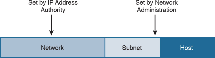
For example, an organization receiving a Class B range of IP addresses, 172.1.0.0/16, could use Subnets to further split the address range. Using 8 bits for the subnet ID, for example, they could create 255 subnets, 172.1.1.0/24, 172.1.2.0/24, 172.1.3.0/24 etc., as shown in Figure 1-49 each with 253 (255 – 2) IP addresses that could be assigned to hosts within the subnet.
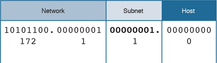
There are two fundamental rules when using subnets in the IP address architecture:
![]() Hosts within the same subnet should be assigned only IP addresses provided by the host portion of that subnet.
Hosts within the same subnet should be assigned only IP addresses provided by the host portion of that subnet.
![]() Traffic between subnets needs a router or a Layer 3 device to flow. This is because each subnet represents a broadcast domain.
Traffic between subnets needs a router or a Layer 3 device to flow. This is because each subnet represents a broadcast domain.
So how do you know how a network has been subnetted? You use network masks. In the case of subnets, the network mask would set all 1s for the network part plus the subnet prefix, while the host part would be all 0s. For example, each subnet derived from the Class B network in Figure 1-49 would get a network mask of 255.255.255.0, or /24.
Variable-Length Subnet Mask (VLSM)
Classic subnetting splits a network into equal parts. This might not be completely efficient because, for example, one subnet may require fewer IP addresses than others. Let’s suppose we have three subnets: SubA, SubB, and SubC. Each subnet has a different number of devices that require an IP address, as shown in Figure 1-50.
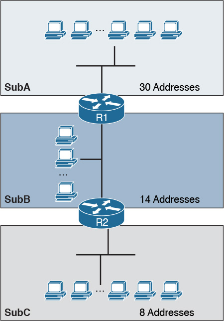
Let’s assume that the subnets have the following requirements in terms of IP addresses:
![]() SubA requires 30 IP addresses.
SubA requires 30 IP addresses.
![]() SubB requires 14 IP addresses.
SubB requires 14 IP addresses.
![]() SubC requires eight IP addresses.
SubC requires eight IP addresses.
Because of the requirement of SubA, in classic subnetting, we would use a subnet mask of /27 so that 30 hosts can be assigned an IP address. However, all the other subnets will also receive a /27 address because of the fixed way a subnet is split. For example, we would create and assign the addresses and subnets as detailed in Table 1-10.
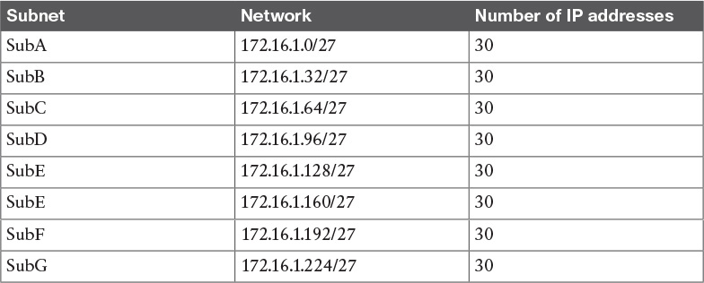
The first subnet, SubA, will consume all the IP addresses; however, SubB will only use 14 out of the 30 provided, SubC will only use eight out of 30, and SubD through SubG will be unused, thus wasting 30 IP addresses each.
The variable-length subnet mask (VLSM) method allows you to subnet a network with subnets of different sizes. The size will be calculated based on the actual need for IP addresses in each subnet. Table 1-11 shows how the VLSM approach can be used in our example. SubA will still need 30 hosts, so it will keep the former subnet mask. SubB only needs 14 IP addresses, so it can use a /28 subnet mask, which allows for up to 14 IP addresses. SubC needs eight IP addresses, so it will also use a /28 subnet mask, because a /29 subnet mask would allow only six IP addresses—that is, 8 – 2 (for the network and broadcast addresses). There is no need to create other subnets, which further saves IP addresses.
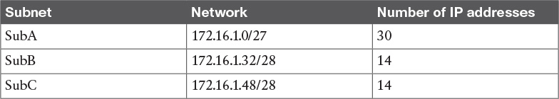
Public and Private IP Addresses
Based on the discussion so far, it is probably clear that IP addresses are scarce resources and that reducing the number of unused IP addresses is a priority due to the exponential growth of the use of TCP/IP and the Internet. CIDR, subnets, and VLSM have greatly helped with optimizing the IP addressing architecture, but by themselves have not been enough to handle the amount of requests for IP addresses.
In most organizations, probably not all the devices need to be reachable from the Internet. Some or even most of them just need to be reached within the organization. For example, an internal database might need to be reached by applications within the organization boundaries, but there is no need to make it accessible for everyone on the Internet.
A private IP addresses range is a range that can be used by any organization without requiring a specific assignment from an IP address assignment authority. The rule is, however, that these ranges can be used only within the organization and should never be used to send traffic over the Internet.
Figure 1-51 shows two organizations using IP address ranges. RFC 1918 defines three IP address ranges for private use:
![]() 10.0.0.0/8 network
10.0.0.0/8 network
![]() 172.16.0.0/12 network
172.16.0.0/12 network
![]() 192.168.0.0/16 network
192.168.0.0/16 network
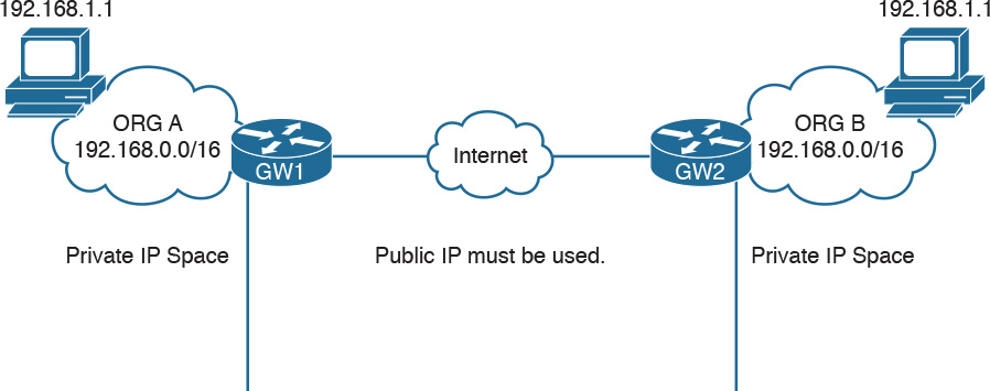
Be careful not to confuse these address ranges with Class A, B, or C because the network masks are different.
Organizations can pick one of these ranges and assign IP addresses internally (for example, using classic subnetting or VLSM). You may have noticed that when you connect to your home router (for example, over Wi-Fi), you may get an IP address that looks like 192.168.x.x. This is because your home router is using the 192.168.0.0/16 network to provide addresses for the local LAN.
Because two organizations can use the same network range, there could be two devices with the same IP address within these two organizations. What if these two devices want to send and receive traffic to and from each other? Recall that we said that private IP addresses should never be used on the Internet. So how can a host with a private IP address browse a web server on the Internet?
The method that is used to solve this problem is network address translation (NAT). NAT uses the concept of a local IP address and a global (or public) IP address. The local IP address is the IP address assigned to a host within the organization, and it is usually a private address. Other devices within the organization will use this address to communicate with that device. The global IP address is the IP address used outside the organization, and it is a public IP address.
NOTE
Two hosts are not permitted to have the same IP address within a subnet. If, within an organization, two hosts have the same IP address, then NAT needs to be performed within the organization to allow traffic.
The following example shows how NAT is used to allow communication between two hosts with the same IP address belonging to two different organizations (see Figure 1-52):
Step 1. Host A initiates the traffic with the source IP address 192.168.1.1, which is the local IP address, and the destination 2.2.2.2, which is the global IP address of Host B.
Step 2. When the packet reaches the Internet gateway of Organization A, the router notices that Host A needs to reach a device on the Internet. Therefore, it will perform an address translation and change the source IP address of the packet with the global IP address of Host A (for example, to 1.1.1.1). This is needed because the 192.168.1.1 address is only locally significant and cannot be routed over the Internet.
Step 3. The Internet gateway of Organization B receives a packet for Host B. It notices that this is the global IP address of Host B, so it will perform an address translation and change the destination IP address to 192.168.1.1 which is the local IP address for Host B.
Step 4. If Host B replies, it will send a packet with the source IP address of its local IP address, 192.168.1.1, and a destination of the global IP address of Host A (1.1.1.1). The Internet gateway at Organization B would follow a similar process and translate the source IP address of the packet to match the global IP address of Host B.
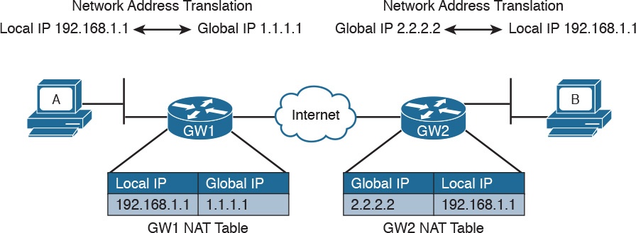
Figure 1-52 Using NAT to Allow Communication Between Two Hosts with the Same IP Addresses Belonging to Two Different Organizations
How do Internet gateways know about the link between global and local IP addresses? The information is included in a table, which is called the NAT table. This is a simple example of how NAT works. NAT is described in more detail in Chapter 2, “Network Security Devices and Cloud Services.”
Special and Reserved IPv4 Addresses
Besides the private addresses, additional IPv4 addresses have been reserved and cannot be used to route traffic over the Internet. Table 1-12 provides a summary of IPv4 unicast special addresses based on RFC 6890. For example, 169.254.0.0/16 is used as the link local address and can be used to communicate only within a subnet (that is, it cannot be routed).
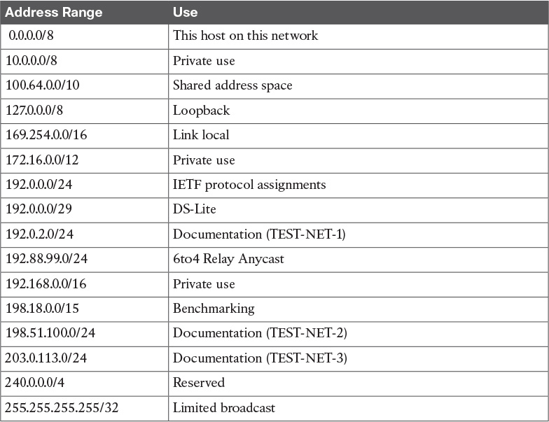
IP Addresses Assignment and DHCP
So far you have learned that each device in a subnet must receive an IP address so it can send and receive IP packets. How do we assign an IP address to a device or interface?
Two methods are available for assigning IP addresses:
![]() Static address assignment: With this method, someone needs to log in to the device and statically assign an IP address and network mask. The advantage of this method is that the IP address will not change because it is statically configured on the device. The disadvantage is that this is a manual configuration. This is typically used on networking devices or on a server where it is important that the IP address is always the same. For example, the following commands can be used to assign an IP address to the F0/0 interface of a Cisco IOS router:
Static address assignment: With this method, someone needs to log in to the device and statically assign an IP address and network mask. The advantage of this method is that the IP address will not change because it is statically configured on the device. The disadvantage is that this is a manual configuration. This is typically used on networking devices or on a server where it is important that the IP address is always the same. For example, the following commands can be used to assign an IP address to the F0/0 interface of a Cisco IOS router:
Interface FastEthernet 0/0
ip address 10.0.0.2 255.255.255.0
![]() Dynamic address assignment: If there are hundreds or thousands of devices, configuring each of them manually is probably not the best use of anyone’s time. Additionally, if for some reason the network administrator changes something in the network mask, network topology, and so on, all devices might need to be reconfigured. Dynamic address assignment allows automatic IP address assignment for networking devices. The Dynamic Host Configuration Protocol (DHCP) is used to provide dynamic address assignment and to provision additional configuration to networking devices. An older protocol not in use anymore and that provided similar services was the BOOTP protocol.
Dynamic address assignment: If there are hundreds or thousands of devices, configuring each of them manually is probably not the best use of anyone’s time. Additionally, if for some reason the network administrator changes something in the network mask, network topology, and so on, all devices might need to be reconfigured. Dynamic address assignment allows automatic IP address assignment for networking devices. The Dynamic Host Configuration Protocol (DHCP) is used to provide dynamic address assignment and to provision additional configuration to networking devices. An older protocol not in use anymore and that provided similar services was the BOOTP protocol.
Let’s explore how DHCP works.
DHCP, which is described in RFC 2131, is a client-server protocol that allows for the automatic provisioning of network configurations to a client device. The DHCP server is configured with a pool of IP addresses that can be assigned to devices. The IP address is not statically assigned to a client, but the DHCP server “leases” the address for a certain amount of time. When the duration of the leasing period is close to expiring, the client can request to renew the leasing. Together with the IP addresses, the DHCP server can provide other configurations.
Here are some examples of network configurations that can be provisioned via DHCP:
![]() IP address
IP address
![]() Network mask
Network mask
![]() Default gateway address
Default gateway address
![]() DNS server address
DNS server address
![]() Domain name
Domain name
DHCP uses UDP as the transport protocol on port 67 for the server and port 68 for the client. DHCP defines several types of messages:
![]() DHCPDISCOVERY: Used by a client to discover DHCP servers within a LAN. It can include some preferences for addresses or lease period. It is sent to the network broadcast address or to the broadcast address 255.255.255.255 and usually carries as a source IP of 0.0.0.0.
DHCPDISCOVERY: Used by a client to discover DHCP servers within a LAN. It can include some preferences for addresses or lease period. It is sent to the network broadcast address or to the broadcast address 255.255.255.255 and usually carries as a source IP of 0.0.0.0.
![]() DHCPOFFER: Sent by a DHCP server to a client. It includes a proposed IP address, called YIADDR, and a network mask. It must also include the server ID, which is the IP address of the server. This is also called SIADDR. There could be multiple DHCP servers within a LAN, so multiple DHCPOFFER messages can be sent in response to a DHCPDISCOVERY.
DHCPOFFER: Sent by a DHCP server to a client. It includes a proposed IP address, called YIADDR, and a network mask. It must also include the server ID, which is the IP address of the server. This is also called SIADDR. There could be multiple DHCP servers within a LAN, so multiple DHCPOFFER messages can be sent in response to a DHCPDISCOVERY.
![]() DHCPREQUEST: Sent from the client to the broadcast network. This message is used to confirm the offer from a particular server. It includes the SIADDR of the DHCP server that has been selected. This is broadcast and not unicast because it provides information to the DHCP servers that have not been chosen about the choice of the client.
DHCPREQUEST: Sent from the client to the broadcast network. This message is used to confirm the offer from a particular server. It includes the SIADDR of the DHCP server that has been selected. This is broadcast and not unicast because it provides information to the DHCP servers that have not been chosen about the choice of the client.
![]() DHCP ACKNOWLEDGEMENT (DHCPACK): Sent from the server to the client to confirm the proposed IP address and other information.
DHCP ACKNOWLEDGEMENT (DHCPACK): Sent from the server to the client to confirm the proposed IP address and other information.
![]() DHCP Not ACKNOWLEDGED (DHCPNACK): Sent from the server to the client in case some issues with the IP address assignment are raised after the DHCPOFFER.
DHCP Not ACKNOWLEDGED (DHCPNACK): Sent from the server to the client in case some issues with the IP address assignment are raised after the DHCPOFFER.
![]() DHCPDECLINE: Sent from the client to the server to highlight that the IP address assigned is in use.
DHCPDECLINE: Sent from the client to the server to highlight that the IP address assigned is in use.
![]() DHCPRELEASE: Sent from the client to the server to release the allocation of an IP address and to end the lease.
DHCPRELEASE: Sent from the client to the server to release the allocation of an IP address and to end the lease.
![]() DHCPINFORM: Sent from the client to the server. It is used to request additional network configuration; however, the client already has an IP address assigned.
DHCPINFORM: Sent from the client to the server. It is used to request additional network configuration; however, the client already has an IP address assigned.
The following steps provide an example of a basic DHCP IP address request (see Figure 1-53):
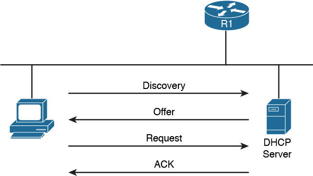
Step 1. When a host first connects to a LAN, it does not have an IP address. It will send a DHCPDISCOVERY packet to discover the DHCP servers within a LAN. In one LAN there could be more than one DHCP server.
Step 2. Each DHCP server responds with DHCPOFFER message.
Step 3. The client receives several offers, picks one of them, and responds with a DHCPREQUEST.
Step 4. The DHCP server that has been selected responds to the client with a DHCPACK to confirm the leasing of the IP address.
What happens if there is no DHCP server within a subnet? To make it work, the Layer 3 device needs to be configured as DHCP relay or DHCP helper. In that case, the router will take the broadcast requests (for example, DHCPDISCOVERY and DHCPREQUEST) and unicast them to the DHCP server configured in the relay, as shown in Figure 1-54. When the DHCP server replies, the router will forward it to the client.
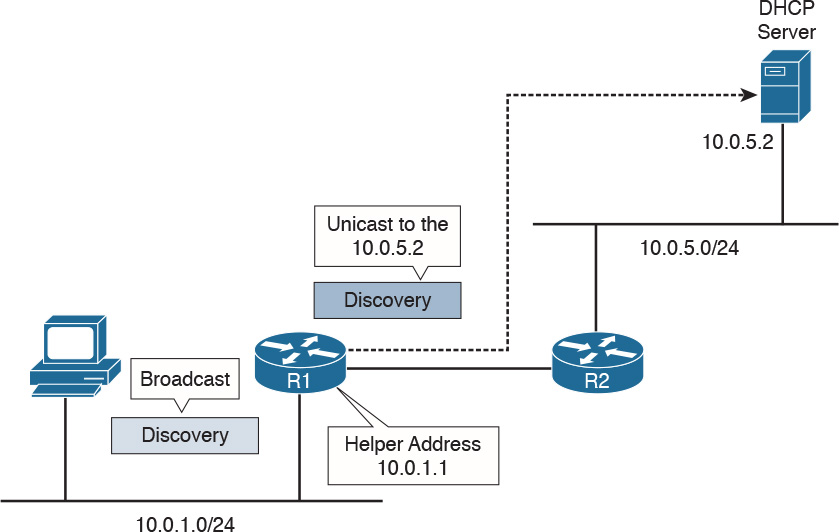
Figure 1-54 shows an example of DHCP relay. The host sends a DHCP DISCOVERY broadcast in the network segment where it is directly connected, 10.0.1.0/24. The router R1 is configured with a helper address, 10.0.1.1, within that subnet. Because of that, R1 picks up the DHCP REQUEST and forwards it to the DHCP server configured. The server will answer the DHCP DISCOVERY with a DHCP OFFER, which is sent directly to the IP helper address of R1. When R1 receives the answer from the DHCP server, it will forward the answer to the host.
IP Communication Within a Subnet and Address Resolution Protocol (ARP)
In the previous section, you learned how each device in a subnet gets its own IP address. So let’s see how devices communicate in a subnet first, and then in the next section we will discuss how devices communicate across multiple subnets. Let’s imagine Host A with IP address 10.0.0.1 wants to communicate with Host B in the same subnet with IP address 10.0.0.3. At this point, Host A knows the IP address of Host B; however, Layer 2 still requires the MAC destination address for Host B. How can Host A get this information? Host A will use the Address Resolution Protocol (ARP) to get the MAC address of Host B.
ARP includes two messages:
![]() ARP request: This is used to request the MAC address given an IP address. It includes the IP address and MAC address of the device sending the request and only the IP address of the destination.
ARP request: This is used to request the MAC address given an IP address. It includes the IP address and MAC address of the device sending the request and only the IP address of the destination.
![]() ARP reply: This is used to provide information about a MAC address. It includes the IP address and MAC address of the device responding to the ARP request and the IP address and MAC address of the device that sent the ARP request.
ARP reply: This is used to provide information about a MAC address. It includes the IP address and MAC address of the device responding to the ARP request and the IP address and MAC address of the device that sent the ARP request.
When Host A needs to send a message to Host B for the first time, it will send an ARP request message using the Layer 2 broadcast address so that all devices within the broadcast domain receive the request. Host B will see the request and recognize that the request is looking for its IP address. It will respond with an ARP reply indicating its own MAC address. Host A stores this information in an ARP table, so the next time it does not have to go through the ARP exchanges.
Figure 1-55 shows an example of an ARP message exchange.
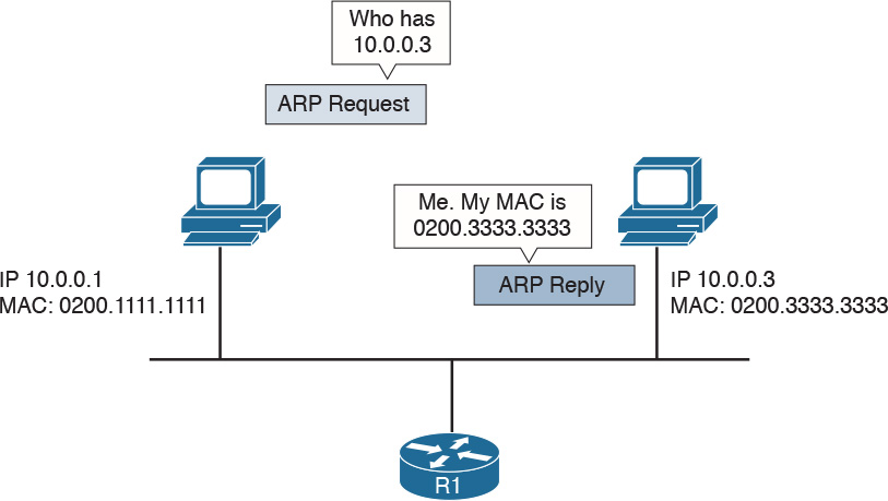
Once the MAC address of the destination is known, Host A can send packets directly to Host B by encapsulating the IP packet within an Ethernet frame, as discussed in the previous sections.
Intersubnet IP Packet Routing
In the previous sections, you learned how IP communication works within a subnet. In this section, we analyze how packets move across subnets. As stated in the previous sections, each subnet is divided by a Layer 3 device (for example, a router). Figure 1-56 shows two hosts, Host A and Host B, which belong to different subnets, and Host C, which is in the same subnet as Host A. The two routers, R1 and R2, provide Layer 3 connectivity, and R3 is the gateway to the rest of the network. The table shown in this figure includes the IP addresses for the relevant interfaces and hosts.
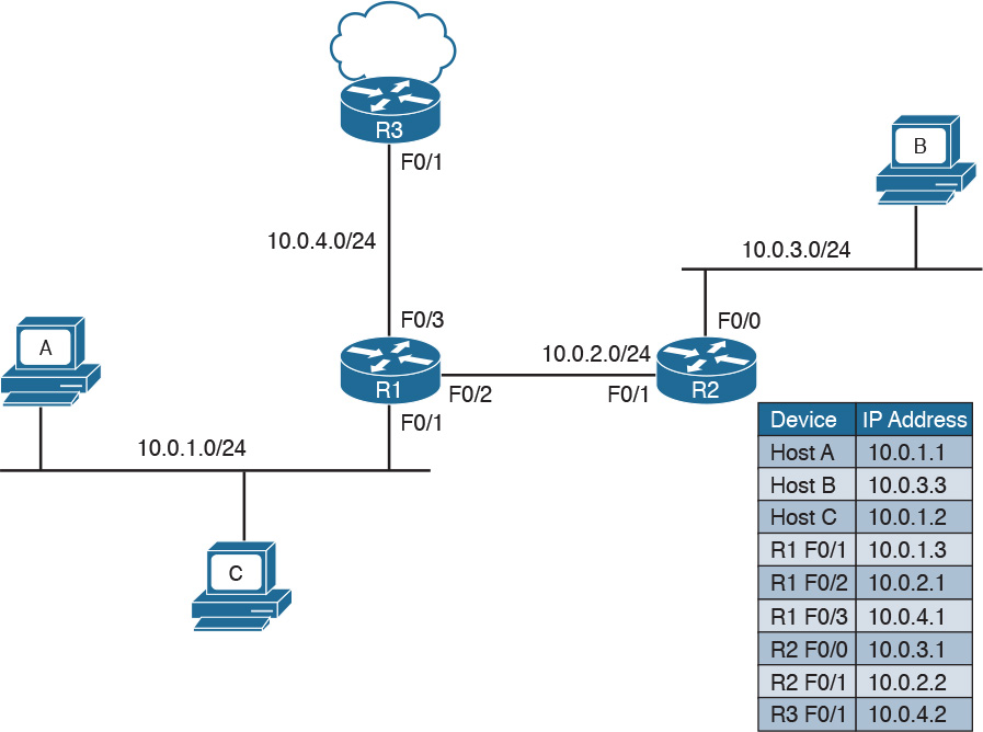
When Host A needs to send a packet, it must make a decision on where to send the packet. The logic implemented by the host is simple:
![]() If the destination IP address is in the same subnet as the interface IP address, the packet is sent directly to the device.
If the destination IP address is in the same subnet as the interface IP address, the packet is sent directly to the device.
![]() If the destination IP address is in a different subnet, it is sent to the default gateway.
If the destination IP address is in a different subnet, it is sent to the default gateway.
The default gateway for a host is the router that allows the packet to exit the host subnet (in this example, R1). The logic is implemented in Host A’s routing table. Host A will see network 10.0.1.1/24 as directly connected and will have an entry saying that packets for any other IP addresses go to the default gateway.
Figure 1-57 shows the routing table for Host A.
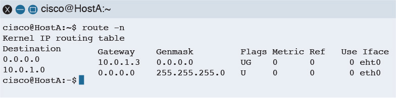
Let’s assume Host A needs to send a packet to Host B; it will check its routing table and decide that the packet’s next hop (which means the next Layer 3 device to handle this packet) is R1 F0/1, with an IP address of 10.0.1.3/24. If Host A does not know the Layer 2 address of R1, it will send an ARP request, as discussed in the previous section.
R1 receives the packets from Host A on the F0/1 interface. At this point, R1 will do a routing table lookup to check where packets with the destination 10.0.3.3 should be sent. Table 1-13 shows what the R1 routing table might look like.
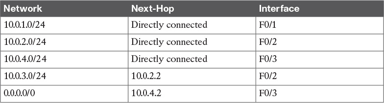
Networks 10.0.1.0/24, 10.0.2.0/24, and 10.0.4.0/24 are directly connected to the router. Network 10.0.3.0/24, which is the network of the destination IP address, has a next hop of R2. The last network, 0.0.0.0/0, is called the default network. This means that, if there is no better match, R1 will send the packet to 10.0.4.2, which is the F0/1 interface of R3. R1 is said to have a default route via R3.
When looking up the routing table, the router will use the interface with the best matching network, which is the network with the longest prefix match. For example, imagine that the router includes the two entries in its routing table outlined in Table 1-14.
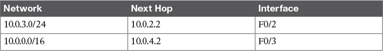
Where would a packet with a destination of IP 10.0.3.3 be sent? In this case, 10.0.3.0/24 is a closer match than 10.0.0.0/16 (longest prefix match), so the router will select 10.0.2.2 via the F0/2 interface.
Let’s go back to our example. R1 identified R2 as the next hop for this packet. R1 will update the IP header information (for example, it will reduce the TTL field by one and recalculate the checksum). After that, it will encapsulate the packet in an Ethernet frame and send it to R2. Remember that R1 does not modify the IP addresses of the packet. When R2 receives the IP packet on F0/1, it will again perform a routing table lookup to understand what to do with the packet. The R2 routing table might look something like Table 1-15.
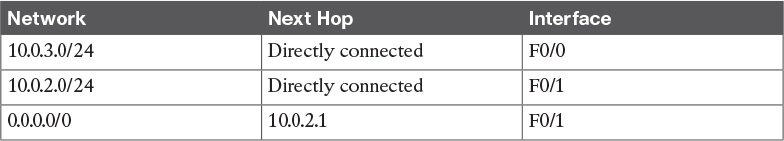
Because the destination IP address matches a directly connected network, R2 can send the packet directly to Host B via the F0/0 interface. If Host B replies to Host A, it will send an IP packet with a destination of IP 10.0.1.1 to R2, which is the default gateway for Host B.
R2 does not have a match for the 10.0.1.1 address; however, it is configured to send anything for which it does not have a match to 10.0.2.1 (R1) via the F0/1 interface. R2 has a default route via R1. R2 will send the packet to R1, which will then deliver to Host A.
Routing Tables and IP Routing Protocols
The routing table is a key component of the forwarding decision. How is this table populated? The connected network will be automatically added when the interface is configured. In fact, the device can determine the connected network from the interface IP address and network mask. The host default gateway can also be configured statically or, as you saw in the “IP Addresses Assignment and DHCP” section, dynamically assigned via DHCP.
For the other entries, there are two options:
![]() Static routes: Routes that have been manually added by the device administrator. Static routes are used when the organization does not use an IP routing protocol or when the device cannot participate in an IP routing protocol.
Static routes: Routes that have been manually added by the device administrator. Static routes are used when the organization does not use an IP routing protocol or when the device cannot participate in an IP routing protocol.
![]() Dynamic routes: Routes that are dynamically learned using an IP routing protocol exchange.
Dynamic routes: Routes that are dynamically learned using an IP routing protocol exchange.
An IP routing protocol is a protocol that allows the exchange of information among Layer 3 devices (for example, among routers) in order to build up the routing table and thus allow the routing of IP packets across the network. A routed protocol is the protocol that actually transports the information and allows for packet forwarding. For example, IPv4 and IPv6 are routed protocols.
Each routing protocol has two major characteristics that need to be defined by the protocol itself:
![]() How and which type of information is exchanged, and when it should be exchanged
How and which type of information is exchanged, and when it should be exchanged
![]() What algorithm is used by each device to calculate the best path to destination
What algorithm is used by each device to calculate the best path to destination
This book does not go into the details of all the routing protocols available; however, it is important that you are familiar at least with the basic functioning of how an IP routing protocol works.
The first classification of a routing protocol is based on where it operates in a network:
![]() Interior gateway protocols (IGPs) operate within the organization boundaries. Here are some examples of IGPs:
Interior gateway protocols (IGPs) operate within the organization boundaries. Here are some examples of IGPs:
![]() Open Shortest Path First (OSPF)
Open Shortest Path First (OSPF)
![]() Intermediate System to Intermediate System (IS-IS)
Intermediate System to Intermediate System (IS-IS)
![]() Enhanced Interior Gateway Routing Protocol (EIGRP)
Enhanced Interior Gateway Routing Protocol (EIGRP)
![]() Routing Information Protocol Version 2 (RIPv2)
Routing Information Protocol Version 2 (RIPv2)
![]() Exterior gateway protocols (EGPs) operate between service providers or very large organizations. An example of an EGP is the Border Gateway Protocol (BGP).
Exterior gateway protocols (EGPs) operate between service providers or very large organizations. An example of an EGP is the Border Gateway Protocol (BGP).
An autonomous system (AS) is a collection of routing information under the administration of a single organization entity. Usually the concept coincides with a single organization. Each AS is identified by an AS number (ASN). IGPs run within an autonomous system, whereas EGPs run across autonomous systems.
Figure 1-58 shows an example of autonomous systems interconnected with EGPs and running IGPs inside.
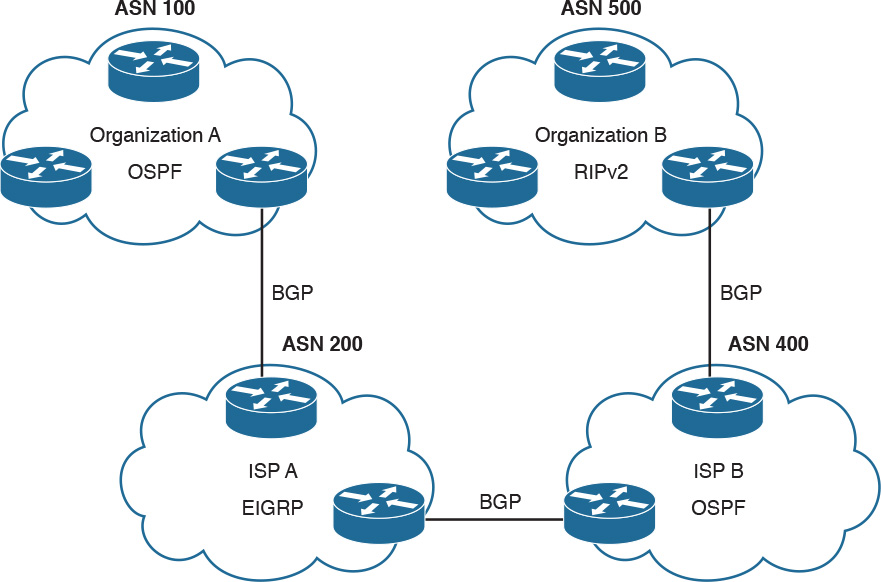
The other common way of classifying IP routing protocols is based on the algorithm used to learn routes from other devices and choose the best path to a destination. The most common algorithms for IGP protocols are distance vector (used in RIPv2), link-state (used in OSPF or IS-IS), and advanced distance vector (also called hybrid, used in EIGRP).
Distance Vector
Distance vector (DV) is one of the first algorithms used for exchanging routing information, and it is usually based on the Bellman-Ford algorithm. The most well-known IP routing protocol using DV is RIPv2. To better understand how DV works, let’s introduce two concepts:
![]() Neighbors are two routers or Layer 3 devices that are directly connected.
Neighbors are two routers or Layer 3 devices that are directly connected.
![]() Hop count is a number that represents the distance (that is, the number of routers on the path) between a router and a specific network.
Hop count is a number that represents the distance (that is, the number of routers on the path) between a router and a specific network.
A device running a DV protocol will send a “vector of distances,” which is a routing protocol message to the neighbors, that contains the information about all the networks the device can reach and the cost.
In Figure 1-59, R2 will send a message to R1 saying that it can reach NetB 10.0.3.0/24 with a cost of 0, because it is directly connected, while it can reach NetC 10.0.5.0/24 with a cost of 1. R3 also sends a message to R1 saying that it can reach NetC 10.0.5.0/24 with a cost of 2 and NetB 10.0.3.0/24 with a cost of 1. R1 receives the information and updates its routing table. It will add both NetB and NetC as reachable via R2 because it has the lowest hop count to the destinations.
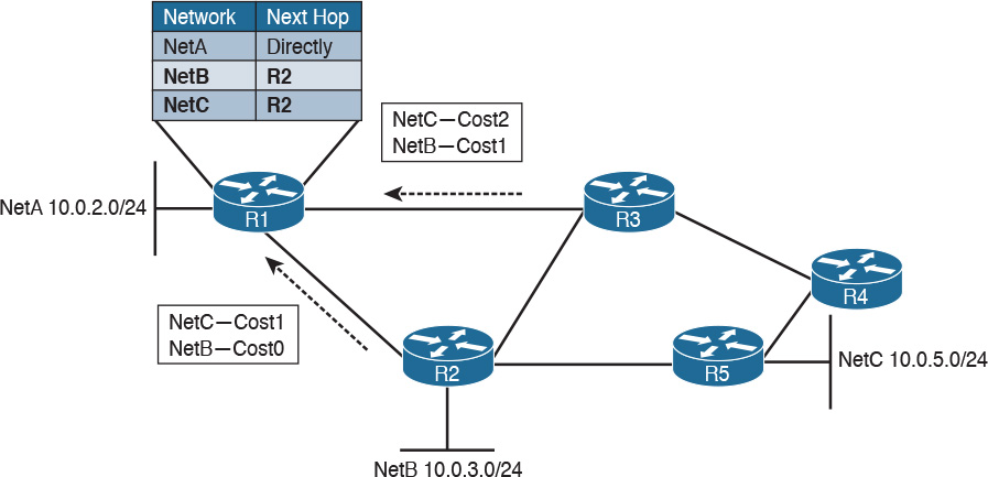
The exchange continues until all routers have a stable routing table. At this point, the routing protocol has converged. Neighbor routers also exchange periodic messages. If the link to a neighbor goes down, both router will detect the situation and inform the other neighbors about the situation. Each neighbor will inform its own neighbors, and the routing tables will be updated accordingly until the protocol converges again.
There are several issues with DV protocols:
![]() Using hop count as the cost to determine the best path to a destination is not the best method. For example, you may have three routers operating with a bandwidth of 1 Gbps and two routers operating with a bandwidth of 1 Mbps. It is probably better for the packet to travel through one more router but with a better bandwidth.
Using hop count as the cost to determine the best path to a destination is not the best method. For example, you may have three routers operating with a bandwidth of 1 Gbps and two routers operating with a bandwidth of 1 Mbps. It is probably better for the packet to travel through one more router but with a better bandwidth.
![]() Routers do not have full visibility into the network topology (they know only what the neighbor routers tell them), so calculating the best path might not be optimal.
Routers do not have full visibility into the network topology (they know only what the neighbor routers tell them), so calculating the best path might not be optimal.
![]() Each update includes an exchange of the full list of networks and costs, which can consume bandwidth.
Each update includes an exchange of the full list of networks and costs, which can consume bandwidth.
![]() It is not loop free. Because of how the algorithm works, in some scenarios packets might start looping in the network. This problem is known as count to infinity. To solve this issue, routing protocols based on DV implement split-horizon and reverse-poison techniques. These techniques, however, increase the time the routing protocol takes to converge to a stable situation.
It is not loop free. Because of how the algorithm works, in some scenarios packets might start looping in the network. This problem is known as count to infinity. To solve this issue, routing protocols based on DV implement split-horizon and reverse-poison techniques. These techniques, however, increase the time the routing protocol takes to converge to a stable situation.
Advanced Distance Vector or Hybrid
To overcome most of the downside of legacy DV protocols such as RIPv2, there is a class of protocols that are based on DV but that implement several structural modifications to the protocol behavior. These are sometimes called advanced distance vector or hybrid protocols, and one of the most known is Cisco EIGRP.
Figure 1-60 shows an example of an EIGRP message exchange between two neighbors. At the beginning, the two routers discover each other with Neighbor Discovery hello packets. Once neighborship is established, the two routers exchange the full routing information, in a similar way as in DV. When an update is due (for example, because of a topology change), only specific information is sent rather than the full update.
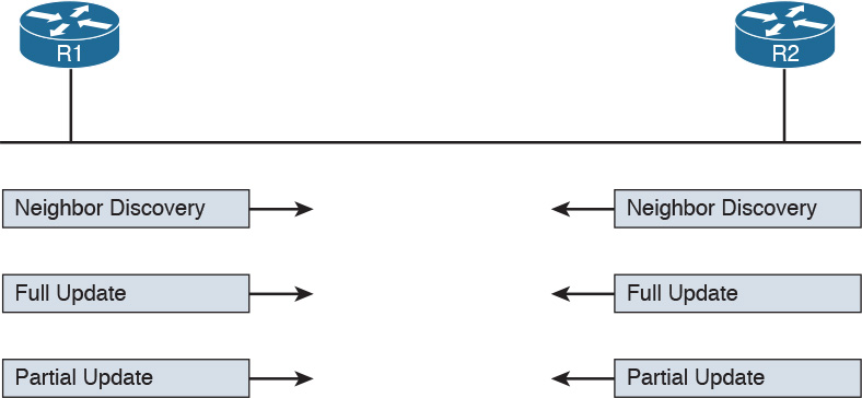
Here are the main enhancements of these types of protocols:
![]() They do not use hop count as a metric to determine the best path to a network. Bandwidth and delay are typically used to determine the best path; however, other metrics can be used in combination, such as load on the link and the reliability of the link.
They do not use hop count as a metric to determine the best path to a network. Bandwidth and delay are typically used to determine the best path; however, other metrics can be used in combination, such as load on the link and the reliability of the link.
![]() The full database update is only sent at initialization, and partial updates are sent in the event of topology changes. This reduces the bandwidth consumed by the protocol.
The full database update is only sent at initialization, and partial updates are sent in the event of topology changes. This reduces the bandwidth consumed by the protocol.
![]() They include a more robust method to avoid loops and reduce the convergence time. For example, EIGRP routers maintain a partial topology table and include an algorithm called Diffused Update Algorithm (DUAL), which is used to calculate the best path to a destination and provides a mechanism to avoid loops.
They include a more robust method to avoid loops and reduce the convergence time. For example, EIGRP routers maintain a partial topology table and include an algorithm called Diffused Update Algorithm (DUAL), which is used to calculate the best path to a destination and provides a mechanism to avoid loops.
Link-State
Link-state algorithms operate in a totally different way than DV, and the fundamental difference is that devices that participate in an IP routing protocol based on a link-state algorithm will have a full view of the network topology; therefore, they can use an algorithm such as Dijkstra or Shortest Path First (SPF) to calculate the best path to each network. The most well-known IP routing protocols using link-state are OSPF and IS-IS.
This section describes the basic functioning of link-state by using OSPF as the basis for the examples. In link-state routing protocols, the concept of router neighbors is maintained while the cost to reach a specific network is based on several parameters. For example, in OSPF, the higher the bandwidth, the lower the cost.
During the initiation phase, each router will send a link-state advertisement (LSA) to the neighbors, which will then forward it to all other neighbors. In Figure 1-61, R2 will send an LSA containing information about its directly connected network and the cost to R1, R3, and R5. Both R3 and R5 will forward this information to their neighbor routers (in this case, R1 and R4). This process is called LSA flooding.
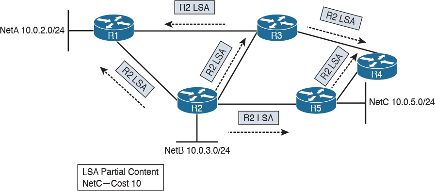
Each router will collect all the LSAs and store them in a database called a link-state database (LSDB).
In this example, R1 receives the same LSA from both R2 and R3. Because there is already one LSA present in the R1 LSDB from R2, the one received from R3 is discarded. At the end of the flooding process, each router should have an identical view of the network topology.
A router can now use an SPF algorithm to calculate the best way to reach each of the networks. Once that is done, the information is added to the router’s routing table. When a link goes down, the neighbor routers that detect it will again flood an LSA with the updated information. Each router will receive the LSA, update the LSDB with that information, recalculate the best path, and update the routing table accordingly.
Advantages of a link-state algorithm include the following:
![]() A better way to calculate the cost to a destination
A better way to calculate the cost to a destination
![]() Less protocol overhead compared to DV because updates do not require sending the full topology
Less protocol overhead compared to DV because updates do not require sending the full topology
![]() Better best-path calculation because each router has a view of the full topology
Better best-path calculation because each router has a view of the full topology
![]() Loop-free
Loop-free
Using Multiple Routing Protocols
An organization can run more than one routing protocol within a network; for example, they can use a combination of static routes and dynamic routes learned via a routing protocol. What happens if the same destination is provided by two routing protocols with a different next hop?
Routers may assign a value, called an administrative distance in Cisco routers, that is used to determine the precedence based on the way the router has learned about a specific network. For example, we may want the router to use the route information provided by OSPF instead of the one provided by RIPv2.
Table 1-16 summarizes the default administrative distance of a Cisco IOS router. These values can be modified to tweak the route selection if needed.
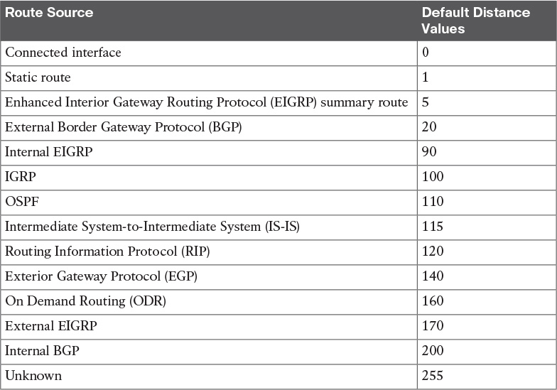
Internet Control Message Protocol (ICMP)
The Internet Control Message Protocol (ICMP) is part of the Internet Protocol suite, and its main purpose is to provide a way to communicate that an error occurred during the routing of IP packets.
ICMP packets are encapsulated directly within the IP payload. An IP packet transporting an ICMP message in its payload sets the Protocol field in the header to 1. The ICMP packet starts with an ICMP header that always includes the Type and Code fields of the ICMP message, which define what that message is used for. ICMP also defines several Message types. Each Message type can include a code.
Table 1-17 provides a summary of the most used values for ICMP Type and Code fields. A full list can be found at http://www.iana.org/assignments/icmp-parameters/icmp-parameters.xhtml.
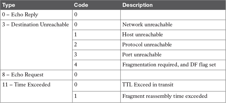
Probably the most known use of an ICMP message is Ping, which is a utility implemented in operating systems using TCP/IP and used to confirm the reachability of a remote host at Layer 3. Ping uses ICMP to perform the task. When you ping a remote destination, an ICMP Echo Request (type 8 code 0) is sent to the destination. If the packet arrives at the destination, the destination sends an ICMP Echo Reply (type 0 code 0) back to the host. This confirms connectivity at Layer 3.
Figure 1-62 shows an example of an ICMP Echo Request and Echo Reply exchange.
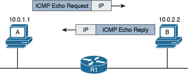
Another very popular ICMP message is Destination Unreachable. This is used for a number of cases, as you can see by the large number of codes for this type. For example, if Host A pings a remote host, but your default gateway does not have information on how to route the packet to that destination, it will send back an ICMP Destination Unreachable – Network Unreachable message (type 3 code 0) back to Host A to communicate that the packet was dropped and could not be delivered.
An ICMP Time Exceeded message is instead generated when a router receives an IP packet with an expired TTL value. The router will drop the packet and send back to the IP packet source an ICMP Time Exceeded – TTL Exceed in Transit message (type 11 code 0).
Domain Name System (DNS)
In all the examples so far, we always had Host A sending a packet to Host B using its IP address. However, having to remember IP addresses is not very convenient. Imagine if you had to remember 72.163.4.161 instead of www.cisco.com when you wanted to browse resources on the Cisco web server.
The solution is called the Domain Name System (DNS). DNS is a hierarchical and distributed database that is used to provide a mapping between an IP address and the name of the device where that IP is assigned.
This section introduces DNS and describes its basic functionalities. DNS works at TCP/IP application layer; however, it is included in this section to complete the overview of how two hosts communicate.
DNS is based on a hierarchical architecture called domain namespace. The hierarchy is organized in a tree structure, where each leaf represents a specific resource and is uniquely identified by its fully qualified domain name (FQDN). The FQDN is formed by linking together the names in the hierarchy, starting from the leaf name up to the root of the tree.
Figure 1-63 shows an example of a DNS domain namespace. The FQDN of the host www.cisco.com is composed, starting from the root, by its top-level domain (TLD), which is com, then the second level domain, cisco, and finally by the resource name or host name, www, which is the name for a server used to provide world-wide web services. Another resource within the same second-level domain could be, for example, a server called tools, in which case the FQDN would be tools.cisco.com.
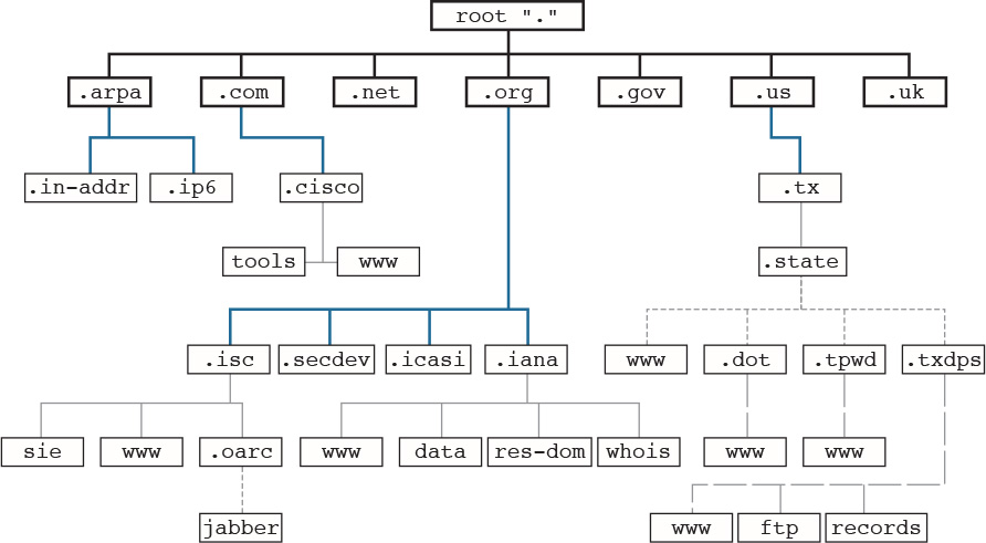
Table 1-18 summarizes the types of domain names.
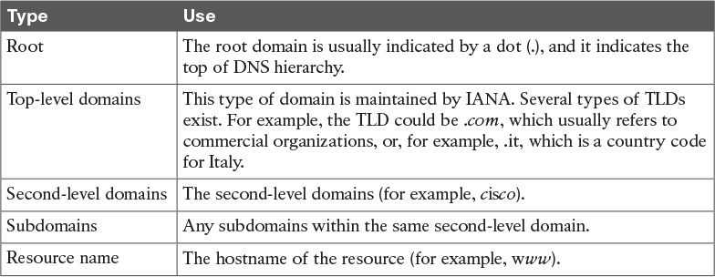
Each entry in the DNS database is called a resource record (RR) and includes several fields. Figure 1-64 shows an example of a resource record structure.
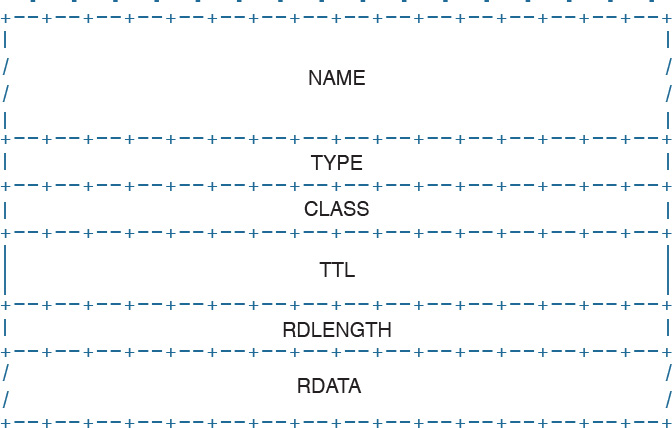
The Type field of the RR indicates which type of resources are included in the RDATA field. For example, the RR type “A” refers to the address record and includes the hostname and the associated IP address. This RR is used for the main functionality of DNS, which is to provide an IP address based on an FQDN.
Table 1-19 summarizes other common RRs.
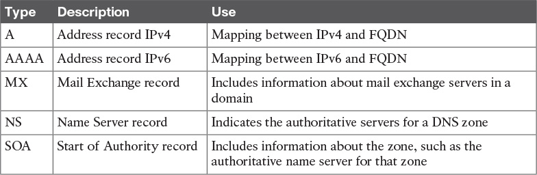
The DNS database is divided into DNS zones. A zone is a portion of the DNS database that is managed by an entity. Each zone must have an SOA RR that includes information about the management of the zone and the primary authoritative name server. Each DNS zone must have an authoritative name server. This server is the one that has the information about the resources present in the DNS zone and can respond to queries concerning those resources.
So how then does Host A get to know the IP address of the www.cisco.com server? The process is very simple. Host A will ask its configured DNS server about the IP address of www.cisco.com. If its DNS knows the answer, it will reply. Otherwise, it will reach the authoritative DNS server for www.cisco.com to get the answer. Let’s see the process in a bit more detail.
Host A needs to query the DNS database to find the answer. In the context of DNS, Host A, or in general any entity that requests a DNS service, is called a DNS resolver. The DNS resolver sends queries to its own DNS server that is configured (for example, via DHCP), as in the previous section.
There are two types of DNS queries, sometimes called lookups:
![]() Recursive queries
Recursive queries
![]() Iterative queries
Iterative queries
Recursive queries are sent from the DNS resolver to its own DNS server. Iterative queries are sent from the DNS server to other DNS servers in case the initial DNS server does not have the answer to the recursive query.
Figure 1-65 shows an example of the DNS resolution process, as detailed in the following steps:
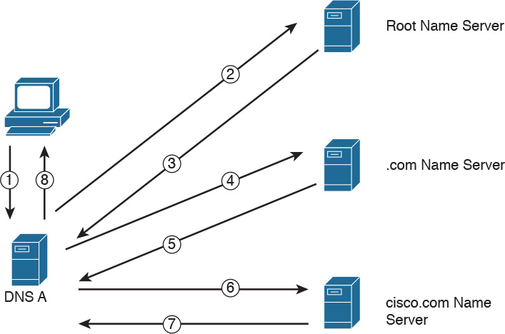
Step 1. Host A sends a recursive DNS query for a type A record (remember, a type A RR is used to map IPv4 IP addresses to FQDN) to resolve www.cisco.com to its own DNS server, DNS A.
Step 2. DNS A checks its DNS cache but does not find the information, so it sends an iterative DNS query to the root DNS server, which is authoritative for all of the Internet.
Step 3. The root DNS server is not authoritative for that host, so it sends back a referral to the .com DNS server, which is the authoritative server for the .com domain.
Steps 4 and 5. The .com DNS server performs a similar process and sends a referral to the cisco.com DNS server.
Steps 6 and 7. The cisco.com DNS server is the DNS authoritative server for www.cisco.com, so it can reply to DNS A with the information.
Step 8. DNS A receives the information and stores it in its DNS cache for future use. The information is stored in the cache for a finite time, which is indicated by the Time To Live (TTL) value in the response from the cisco.com DNS server. DNS A can now reply to the recursive DNS query from Host A.
Host A receives the information from DNS A and can start sending packets to www.cisco.com using the correct IP address. Additionally, it will store the information in its own DNS cache for a time indicated in the TTL field.
The DNS protocol, described in RFC 1035, uses one message format for both queries and replies. A DNS message includes five sections: Header, Question, Answer, Authority, and Additional.
The DNS protocol can use UDP or TCP as the transport protocol, and the DNS server is typically listening on port 53 for both UDP and TCP. According to RFC 1035, UDP port 53 is recommended for standard queries, whereas TCP is used for DNS zone transfer.
IPv6 Fundamentals
So far we have analyzed how two or more hosts can communicate using a routed protocol (for example, IP), mainly using IPv4. In this section, we cover the newer version of the IP protocol: IPv6.
With the growth of the Internet and communication networks based on TCP/IP, the number of IPv4 addresses quickly became a scarce resource. Using private addressing with NAT or CIDR has been fundamental to limiting the impact of the issue; however, a long-term solution was needed. IPv6 has been designed with that in mind, and its main purpose is to provide a larger IP address space to support the growth of the number of devices needing to communicate using the TCP/IP model.
Most of the concepts we have discussed in the sections on the Internet Protocol and Layer 3 technologies, such as the routing of a packet and routing protocols, work in a similar way with IPv6. Of course, some modifications need to be taken into account due to structural differences with IPv4 (for example, the IP address length).
This book will not go into detail on the IPv6 protocol; however, it is important that security professionals and candidates for the CCNA Cyber Ops SECFND certification have a basic understanding of IPv6 address, how IPv6 works, and its differences and commonalities with IPv4.
Table 1-20 summarizes the main differences and commonalities between IPv6 and IPv4.
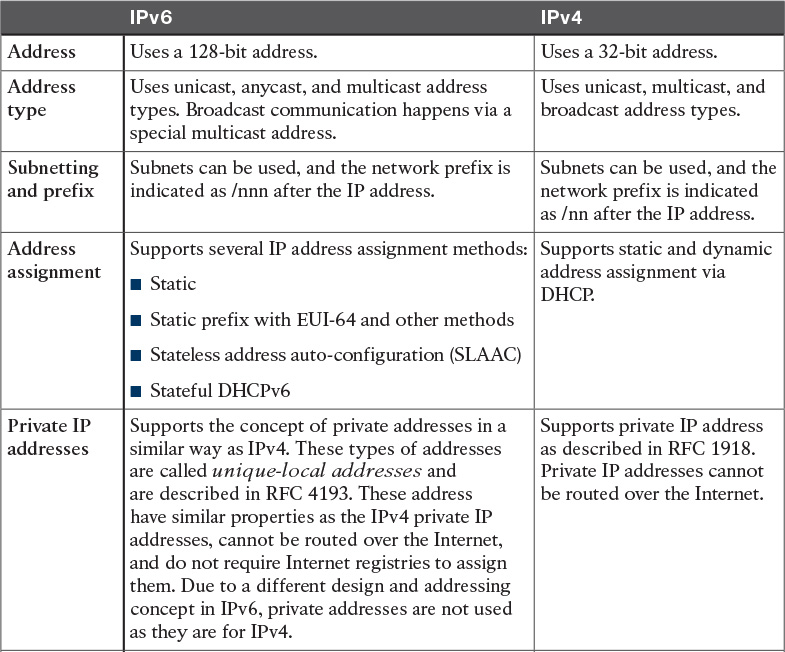
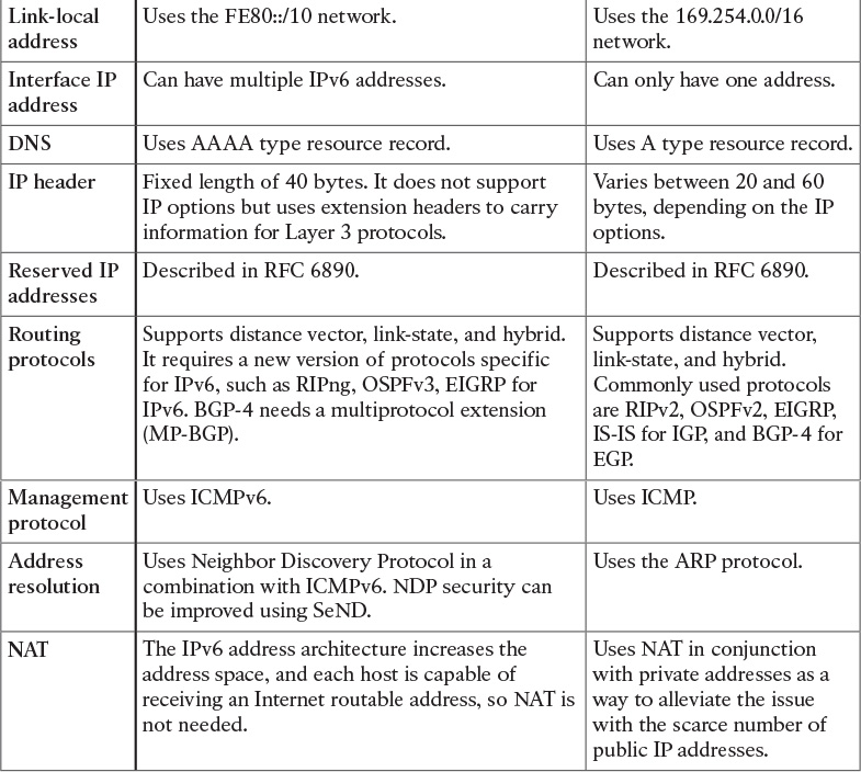
Figure 1-66 shows an example of communications between Host A and Host B using IPv6. Similar to the example we saw in the IPv4 section, Host A and Host B would have an IP address that can identify the device at Layer 3. Each router interface would also have an IPv6 address.
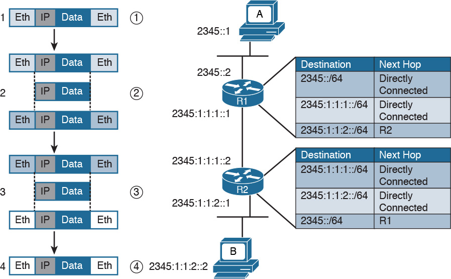
Host A will send the IPv6 packet encapsulated in an Ethernet frame to its default gateway, R1 (step 1).
R1 decapsulates the IPv6 packet, looks up the routing table, and finds that the next hop is R2. It encapsulates the packet in a new Layer 2 frame and sends it to R2 (step 2). R2 will follow a similar process and finally deliver the packet to Host B.
In the example in Figure 1-66, probably the most notable difference is the format of the IPv6 address. However, there are additional differences that are not visible. For example, how does an IPv6 host know about the default gateway? Is ARP needed to find out the MAC address given an IP address for intra-subnet traffic?
As discussed at the beginning of this section, several protocols that work for IPv4 could work with IPv6 with just a few modifications. Some others are not necessary with IPv6, and some new protocols had to be created. For example, ICMP and DHCP could not be used “as is,” so new versions have been created: ICMPv6 and DHCPv6. The functionality of ARP has been replaced with a new protocol called IPv6 Neighbor Discovery. OSPF, EIGRP, and other routing protocols have been modified to work with IPv6, and new versions have been proposed, such as OSPFv3, EIGRPv6, and RIPng.
IPv6 Header
IPv6 has been designed to provide similar functionality to IPv4; however, it is actually a separate and new protocol rather than an improvement to IPv4. As such, RFC 2460 defines a new header for IPv6 packets.
Figure 1-67 shows an IPv6 header.
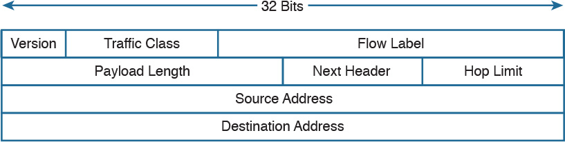
Most of the fields serve the same purpose as their counterparts in IPv4.
With IPv6, one of the core differences with IPv4 is the introduction of extension headers. Besides the fixed header, shown in Figure 1-67, IPv6 allows additional headers to carry information for Layer 3 protocols. The extension header is positioned just after the fixed header and before the IPv6 packet payload. The Next Header field in the IPv6 header is used to determine what the next header in the packet is. If no extension headers are present, the field will point to the Layer 4 header that is being transported (for example, the TCP header). This is similar to the IP protocol field in IPv4. If an extension header is present, it will indicate which type of extension header will follow.
IPv6 allows the use of multiple extension headers in a chained fashion. Each extension header contains a Next Header field that is used to determine whether an additional extension header follows. The last extension header in the chain indicates the Layer 4 header type being transported (for example, TCP).
Figure 1-68 shows examples of chained extension headers. The first shows an IPv6 header without any extension headers. This is indicated by the Next Header field set to TCP. In the third example of Figure 1-68, instead, the IPv6 header is followed by two extension headers: the Routing extension header and the Fragmentation extension header. The Fragmentation header’s Next Header field is indicating that a TCP header will follow.
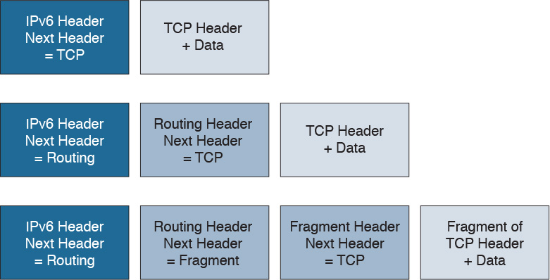
IPv6 Addressing and Subnets
The most notable difference between IPv4 and IPv6 is the IP address and specifically the IP address length. The IPv6 address is 128 bits long, whereas the IPv4 address is only 32 bits. This is because IPv6 is aimed at increasing the IP address space to resolve the IPv4 address exhaustion issue and cope with the growth in demand of IP addresses. Similar to IPv4, writing an IPv6 address in binary is not convenient. IPv6 uses a different convention than IPv4 when it comes to writing down the IP address.
IPv6 addresses are represented by using four hexadecimal digits, which represent 16 bits, followed by a colon (:) An example of an IPv6 address is as follows:
2340:1111:AAAA:0001:1234:5678:9ABC:1234
Some additional simplification can be done to reduce the complexity of writing down an IPv6 address:
![]() For each block of four digits, the leading zeros can be omitted.
For each block of four digits, the leading zeros can be omitted.
![]() If two or more consecutive blocks of four digits are 0000, they can be substituted with two colons (::). This, however, can only happen one time within an IPv6 address.
If two or more consecutive blocks of four digits are 0000, they can be substituted with two colons (::). This, however, can only happen one time within an IPv6 address.
Let’s use FE00:0000:0000:0001:0000:0000:0000:0056 as an example. The first rule will transform it as follows:
FE00:0:0:1:0:0:0:56
The second rule can be applied either to the second and third blocks or to the fifth, sixth, and seventh blocks, but not to both. The shortest form would be to apply it to the fifth, sixth, and seventh blocks, which results in the following:
FE00:0:0:1::56
Like IPv4, IPv6 supports prefix length notation to identify subnets. For example, an address could be written as 2222:1111:0:1:A:B:C:D/64, where the /64 indicates the prefix length. To find the network ID, you can use the same process we used for IPv4; that is, you can take the first n bits (in this case, 64) from the IPv6 address and set the remaining bits to zeros. Figure 1-69 illustrates the process.
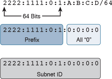
The resulting IPv6 address indicates the prefix or network for that IPv6 address. In our example, this would be 2222:1111:0:1:0:0:0:0 or 2222:1111:0:1::.
IPv6 also defines three types of addresses:
![]() Unicast: Used to identify one specific interface.
Unicast: Used to identify one specific interface.
![]() Anycast: Used to identify a set of interfaces (for example, on multiple nodes). When this address is used, packets are usually delivered to the nearest interface with that address.
Anycast: Used to identify a set of interfaces (for example, on multiple nodes). When this address is used, packets are usually delivered to the nearest interface with that address.
![]() Multicast: Used to identify a set of interfaces. When this address is used, packets are usually delivered to all interfaces identified by that identifier.
Multicast: Used to identify a set of interfaces. When this address is used, packets are usually delivered to all interfaces identified by that identifier.
In IPv6, there is no concept of broadcast address as we have seen for IPv4. To send packets in broadcast, IPv6 uses a multicast address. Several types of addresses are defined within these three main classes. In this book, we will not analyze all types of addresses and instead will focus on two particular types defined within the Unicast class: global unicast and link-local unicast addresses (LLA).
In very simple terms, the difference between global unicast and link-local unicast is that the former can be routed over the Internet whereas the latter is only locally significant within the local link, and it is used for specific operations such as for the Neighbor Discovery Protocol process.
One concept that is unique for IPv6 is that one interface can have multiple IPv6 addresses. For example, the same interface can have a link-local and a global unicast address. Actually, this is one of the most common cases. In fact, IPv6 mandates that all interfaces have at least one link-local address.
The global unicast address is very similar to a public IPv4 address. A global unicast IPv6 address can be split in three parts (or prefixes), as shown in Figure 1-70.
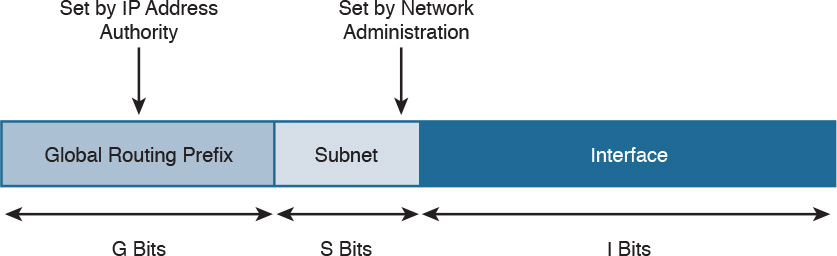
The first one is called the global routing prefix and identifies the address block, as assigned to an organization, the subnet ID, used to identify a subnet within that block space, and the interface ID, which identifies an interface within that subnet.
The assignment of the global routing prefix is provided by IANA or by any of its delegation, such as a regional Internet registry organization. The subnet part is decided within the organization and is based on the IP address schema adopted.
The link-local address (LLA) is a special class of unicast address that is only locally significant within a link or subnet. In IPv6, at least one LLA needs to be configured per interface. The LLA is used for a number of functions, such as by the Neighbor Discovery Protocol or as the next-hop address instead of the global unicast address. Any IPv6 packet that includes an LLA should not be forwarded by a router outside of the subnet.
An LLA address should always start with the first 10 bits set to 1111111010 (FF80::/10), followed by 54 bits set to all 0s. This means that an LLA address always starts with FE80:0000:0000:0000 for the first 64 bits, and the interface ID is determined by the EUI-64 method, which we discuss in the next section.
Figure 1-71 shows an example of an IPv6 LLA.
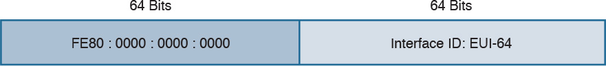
IPv6 multicast addresses are also very important for the correct functioning of IPv6 (for example, because they replace the network broadcast address and are used in a number of protocols to reach other devices). An IPv6 multicast address always starts with the first 8 bits set to 1s, which is equivalent to FF00::/8.
Figure 1-72 shows the format of an IPv6 multicast address.
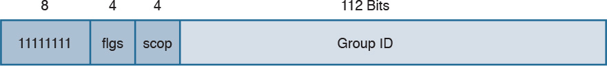
The FLGS and SCOP fields are used to communicate whether the address is permanently assigned (and thus well known) or not, and for which scope the address can be used (for example, only for local-link).
Table 1-21 summarizes some of most common IPv6 multicast addresses. A list of reserved IPv6 multicast addresses can be found at http://www.iana.org/assignments/ipv6-multicast-addresses/ipv6-multicast-addresses.xhtml.
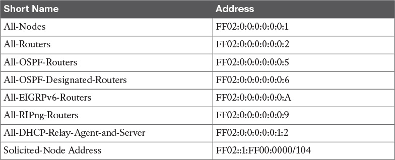
Special and Reserved IPv6 Addresses
Like IPv4, IPv6 includes some reserved addresses that should not be used for interface assignment. Table 1-22 provides a summary of the special and reserved unicast addresses and prefixes for IPv6 based on RFC 6890.
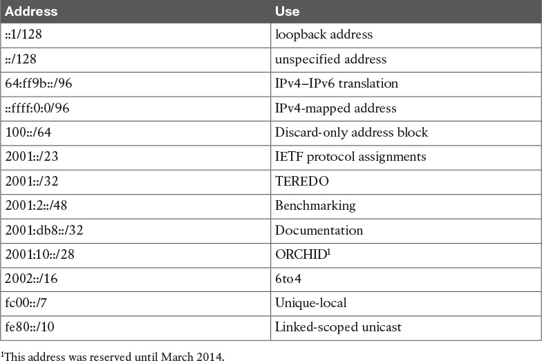
IPv6 Addresses Assignment, Neighbor Discovery Protocol, and DHCPv6
IPv6 supports several methods for assigning an IP address to an interface:
![]() Static
Static
![]() Static prefix with EUI-64 method
Static prefix with EUI-64 method
![]() Stateless address auto-configuration (SLAAC)
Stateless address auto-configuration (SLAAC)
![]() Stateful DHCPv6
Stateful DHCPv6
With static assignment, the IP address and prefix are configured by the device administrator. In some devices, such as Cisco IOS routers, it is possible just to configure the IPv6 prefix, the first 64 bits, and let the router automatically calculate the interface ID portion of the address, the last 64 bits. The method to calculate the interface ID is called the EUI-64 method.
The EUI-64 method, described in RFC 4291, uses the following rules to build the interface ID:
1. Split the interface MAC address in two.
2. Add FFFE in between. This makes the address 64-bits long.
3. Invert the 7th bit (for example, if the bit is 1, write 0, and vice versa).
Figure 1-73 shows an example of the EUI-64 method to calculate the interface ID portion of an IPv6 address. In this example, the MAC address of the interface is 0200.1111.1111. We first split the MAC address and add FFFE in the middle. We then flip the 7th bit from 1 to 0. This results in an interface ID of 0000.11FF.FE11.1111.
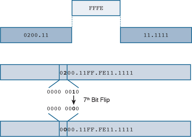
The EUI-64 method is also used to calculate the interface ID for an LLA address, as explained in the previous section.
The third method, SLAAC, allows for automatic address assignment when the IPv6 network prefix and prefix length are not known (for example, if they are not manually configured). To understand how SLAAC works, we need to look at a new protocol that is specific for IPv6: the Neighbor Discovery Protocol (NDP).
NDP is used for several functionalities:
![]() Router discovery: Used to discover routers within a subnet.
Router discovery: Used to discover routers within a subnet.
![]() Prefix discovery: Used to find out the IPv6 network prefix in a given link.
Prefix discovery: Used to find out the IPv6 network prefix in a given link.
![]() Address auto-configuration: Supports SLAAC to provide automatic address configuration.
Address auto-configuration: Supports SLAAC to provide automatic address configuration.
![]() Address resolution: Similar to ARP for IPv4, address resolution is used to determine the link layer address, given an IPv6 address.
Address resolution: Similar to ARP for IPv4, address resolution is used to determine the link layer address, given an IPv6 address.
![]() Next-hop determination: Used to determine the next hop for a specific destination.
Next-hop determination: Used to determine the next hop for a specific destination.
![]() Neighbor unreachability detection (NUD): Used to determine whether a neighbor is reachable. It is useful, for example, to determine whether the next-hop router is still available or an alternative router should be used.
Neighbor unreachability detection (NUD): Used to determine whether a neighbor is reachable. It is useful, for example, to determine whether the next-hop router is still available or an alternative router should be used.
![]() Duplicate address detection (DAD): Used to determine whether the address a node decided to use is already in use by some other node.
Duplicate address detection (DAD): Used to determine whether the address a node decided to use is already in use by some other node.
![]() Redirect: Used to inform nodes about a better first-hop node for a destination.
Redirect: Used to inform nodes about a better first-hop node for a destination.
NDP uses ICMP version 6 (ICMPv6) to provide these functionalities. As part of the NDP specification, five new ICMPv6 messages are defined:
![]() Router Solicitation (RS): This message is sent from hosts to routers and is used to request a Router Advertisement message. The source IP address of this message is either the host-assigned IP address or the unspecified address ::/128 if an IP address is not assigned yet. The destination IP address is the all-routers multicast address FF01::2/128.
Router Solicitation (RS): This message is sent from hosts to routers and is used to request a Router Advertisement message. The source IP address of this message is either the host-assigned IP address or the unspecified address ::/128 if an IP address is not assigned yet. The destination IP address is the all-routers multicast address FF01::2/128.
![]() Router Advertisement (RA): This message is sent from routers to all hosts, and it is used to communicate information such as the IP address of the router and information about network prefix and prefix length, or the allowed MTU. This can be sent at regular intervals or to respond to an RS message.
Router Advertisement (RA): This message is sent from routers to all hosts, and it is used to communicate information such as the IP address of the router and information about network prefix and prefix length, or the allowed MTU. This can be sent at regular intervals or to respond to an RS message.
The source IP of this message is the link-local IPv6 address of the router interface, and the destination is either all-nodes multicast address FF01::1 or the address of the host that sent the RS message.
![]() Neighbor Solicitation (NS): This message is used to request the link-layer address from a neighbor node. It is also used for NUD and DUD functionality. The source IP address would be the IPv6 address of the interface, if already assigned, or the unspecified address ::/128.
Neighbor Solicitation (NS): This message is used to request the link-layer address from a neighbor node. It is also used for NUD and DUD functionality. The source IP address would be the IPv6 address of the interface, if already assigned, or the unspecified address ::/128.
![]() Neighbor Advertisement (NA): This message is sent in response to an NS or can be sent unsolicited to flag a change in the link-layer address. The source IP address is the interface IP, while the destination is either the IP address of the node that sent the NS or the all-nodes address FF01::1.
Neighbor Advertisement (NA): This message is sent in response to an NS or can be sent unsolicited to flag a change in the link-layer address. The source IP address is the interface IP, while the destination is either the IP address of the node that sent the NS or the all-nodes address FF01::1.
![]() Redirect: This message is used to inform the hosts about a better first hop. The source IP address is the link-local IP of the router, and the destination IP address is the IP address of the packet that triggered the redirect.
Redirect: This message is used to inform the hosts about a better first hop. The source IP address is the link-local IP of the router, and the destination IP address is the IP address of the packet that triggered the redirect.
Figure 1-74 shows an example of an RS/RA exchange to get information about the router. In this example, Host A sends a Router Solicitation to all routers in the subnet to get the network prefix and prefix length.
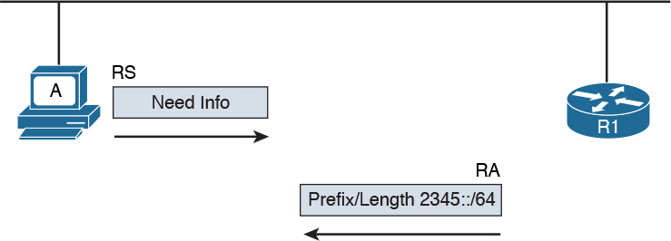
Figure 1-75 shows an example of an NS/NA exchange to get information about the link-layer address. This process replaces the ARP process in IPv4. Host A needs to have the MAC address of Host B so it can send frames. It sends an NS asking who has 2345::2, and Host B responds with an NA, indicating its MAC address.
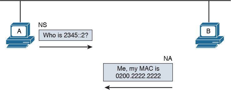
Due to the criticality of the NDP operation, RFC 3971 describes the Secure Neighbor Discovery (SeND) protocol to improve the security of NDP. SeND defines two ND messages—Certification Path Solicitation (CPS) and Certification Path Answer (CPA)—an additional ND option, and an additional auto-configuration mechanism.
Now that you know how NDP works, you can better understand the SLAAC process. In the following example, we assume the host uses the EUI-64 method to generate an LLA. At the start, the host generates an LLA address. This provides link-local connectivity to neighbors.
At this point, the host can receive RAs from the neighbor’s routers, or, optionally, it can solicit an RA by sending an RS message. The RA message contains the network prefix and prefix length information that can be used by the host to create a global unicast IP address.
The prefix part of the address is provided by the information included in the RA. The interface ID, instead, is provided by using EUI-64 or other methods (for example, randomly). This depends on how the host has implemented SLAAC. For example, a host may implement a privacy extension (described in RFC 4941) or a cryptographically generated address (CGA) when SeND is used. Before the address can be finally assigned to the interface, the host can use the DAD functionality of NDP to find out whether any other host is using the same IP.
The following steps detail address assignment via SLAAC. In Figure 1-76, Host A has a MAC address of 0200.2211.1111.
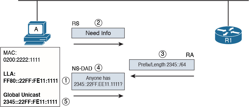
Step 1. The SLAAC process starts by calculating the LLA. This is done by using the EUI-64 method. This will result in an LLA address of FF80::22FF:FE11:1111.
Step 2. At this point, Host A has link-local connectivity and can send an RS message to get information from the local routers.
Step 3. R1 responds with information about the prefix and prefix length, 2345::/64.
Step 4. Host A uses this information to calculate its global unicast address 2345::22FF:FE11:1111. Before using this address, Host A uses DAD to check whether any other device is using the same address. It sends an NS message asking whether anyone is using this address.
Step 5. Since no one responded to the NS message, Host A assumes it is the only one with that address. This terminates the SLAAC configuration.
The fourth method we look at in this section is stateful DHCPv6. As with many other protocols, a new version of DHCP has been defined to make it work with IPv6. DHCP version 6 uses UDP as the transport protocol with port 546 for clients and 547 for servers or relays.
Two modes of operation have been defined:
![]() Stateful DHCPv6: Works pretty much like DHCPv4, where a server assigns IP addresses to clients and can provide additional network configuration. The server keeps track of which IP addresses have been leased and to which clients. The difference is that stateful DHCPv6 does not provide information about the default route; that functionality is provided by NDP.
Stateful DHCPv6: Works pretty much like DHCPv4, where a server assigns IP addresses to clients and can provide additional network configuration. The server keeps track of which IP addresses have been leased and to which clients. The difference is that stateful DHCPv6 does not provide information about the default route; that functionality is provided by NDP.
![]() Stateless DHCPv6: Used to provide network configuration only. It is not used to provide IP address assignment. The term stateless comes from the fact that the DHCPv6 server does not need to keep the state of the leasing of an IPv6 address. Stateless DHCPv6 can be used in combination with static or SLAAC IPv6 assignments to provide additional network configuration such as for a DNS server or NTP server.
Stateless DHCPv6: Used to provide network configuration only. It is not used to provide IP address assignment. The term stateless comes from the fact that the DHCPv6 server does not need to keep the state of the leasing of an IPv6 address. Stateless DHCPv6 can be used in combination with static or SLAAC IPv6 assignments to provide additional network configuration such as for a DNS server or NTP server.
DHCPv6 defines several new messages as well, and some of the messages present in DHCPv4 have been renamed.
The following steps show a basic stateful DHCPv6 exchange for IPv6 address assignment (see Figure 1-77):
Step 1. The client sends a DHCPv6 Solicit message to the IPv6 multicast address All_DHCP_Relay_Agents_and_Servers FF02::1:2 and uses its link-local address as the source.
Step 2. The DHCPv6 servers reply with a DHCPv6 Advertise message back to the client.
Step 3. The client picks a DHCPv6 server and sends a DHCPv6 Request message to request the IP address and additional configuration.
Step 4. The DHCPv6 server sends a DHCPv6 Reply message with the information.
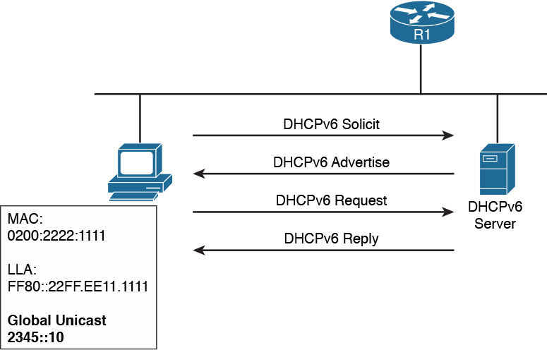
If an IP address has been assigned using a different method, a host can use stateless DHCPv6 to receive additional configuration information. This involves only two messages instead of four, as shown here (see Figure 1-78):
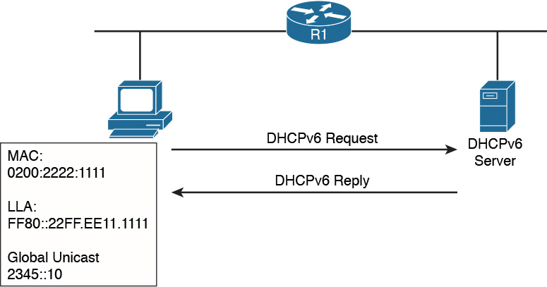
Step 1. The client sends a DHCPv6 Information Request message to the IPv6 multicast address All_DHCP_Relay_Agents_and_Servers FF02::1:2.
Step 2. The server sends a DHCPv6 Reply with the information.
Just like DHCPv4, DHCPv6 includes the relay functionality to allow clients to access DHCPv6 servers outside of a subnet.
Transport Layer Technologies and Protocols
The last concept to discuss in this chapter is how two hosts (Host A and Host B) can establish end-to-end communication. The end-to-end communication service is provided by the transport layer or Layer 4 protocols. These protocols are the focus of this section.
Several protocols work at the transport layer and offer different functionalities. In this section, we focus on two of the most used protocols: User Datagram Protocol (UDP) and Transmission Control Protocol (TCP).
Before we get into the protocol details, we need to discuss the concept of multiplexing, which is at the base of the functionality of UDP and TCP. On a single host, there may be multiple applications that want to use the transport layer protocols (that is, TCP and UDP) to communicate with remote hosts. In Figure 1-79, for example, Host B supports a web server and an FTP server. Let’s imagine that Host A would like to browse and use the FTP services from Host B. It will send two TCP requests to Host B. The question is, how does Host B differentiate between the two requests and forward the packets to the correct application?
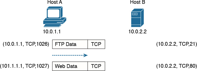
The solution to this problem is provided by multiplexing, which relies on the concept of a socket. A socket is a combination of three pieces of information:
![]() The host IP address
The host IP address
![]() A port number
A port number
![]() The transport layer protocol
The transport layer protocol
The first two items are sometimes grouped together under the notion of a socket address. A socket (in the case of this example, a TCP socket) is formed by the IP address of the host and a port number, which is used by the host to identify the connection. The pair of sockets on the two hosts, Host A and Host B, uniquely identify a transport layer connection.
For example, the Host A socket for the FTP connection would be (10.0.1.1, 1026), where 10.0.1.1 is the IP address of Host A and 1026 is the TCP port used for the communication. The Host B socket for the same connection would be (10.0.2.2, 21), where 21 is the standard port assigned to FTP services.
Similarly, the Host A socket for the HTTP connection (web service) would be (10.0.1.1, 1027), whereas the Host B socket would be (10.0.2.2, 80), where 80 is the standard port assigned to HTTP services.
The preceding example illustrates the concepts of multiplexing and sockets as applied to a TCP connection, but the same holds for UDP. For example, when a DNS query is made to a DNS server, as detailed earlier in the section “Domain Name System (DNS)” of this chapter, a UDP socket is used on the DNS resolver and on the DNS server.
An additional concept that’s generally used to describe protocols at the transport layer is whether a formal connection needs to be established before a device can send data. Therefore, the protocols can be classified as follows:
![]() Connection oriented: In this case, the protocol requires that a formal connection be established before data can be sent. TCP is a connection-oriented protocol and provides connection establishment by using three packets prior to sending data. Generally, connection-oriented protocols have a mechanism to terminate a connection. Connection-oriented protocols are more reliable because the connection establishment allows the exchange of settings and ensures the receiving party is able to receive packets. The drawback is that it adds additional overhead and delay to the transmission of information.
Connection oriented: In this case, the protocol requires that a formal connection be established before data can be sent. TCP is a connection-oriented protocol and provides connection establishment by using three packets prior to sending data. Generally, connection-oriented protocols have a mechanism to terminate a connection. Connection-oriented protocols are more reliable because the connection establishment allows the exchange of settings and ensures the receiving party is able to receive packets. The drawback is that it adds additional overhead and delay to the transmission of information.
![]() Connectionless: In this case, the protocol allows packets to be sent without any need for a connection. UDP is an example of a connectionless protocol.
Connectionless: In this case, the protocol allows packets to be sent without any need for a connection. UDP is an example of a connectionless protocol.
We will now examine how TCP and UDP work in a bit more detail.
Transmission Control Protocol (TCP)
The Transmission Control Protocol (TCP) is a reliable, connection-oriented protocol for communicating over the Internet. Connection oriented means that TCP requires a connection between two hosts to be established through a specific packet exchange before any data packets can be sent. This is the opposite of connectionless protocols (such as UDP), which don’t require any exchange prior to data transmission.
As mentioned in RFC 793, which specifies the TCP protocol, TCP assumes it can obtain simple and potentially unreliable datagrams (IP packets) from lower-level protocols. TCP provides most of the services expected by a transport layer protocol. This section explains the following services and features provided by TCP:
![]() Multiplexing
Multiplexing
![]() Connection establishment and termination
Connection establishment and termination
![]() Reliability (error detection and recovery)
Reliability (error detection and recovery)
![]() Flow control
Flow control
You may wonder why we don’t use TCP for all applications due to these important features. The reason is that the reliability offered by TCP is done at the cost of lower speed and the need for increased bandwidth, in order to manage this process. For this reason, some applications that require fast speed but don’t necessarily need to have all the data packets received to provide the requested level of quality (such as voice/video over IP) rely on UDP instead of TCP.
Table 1-23 summarizes the services provided by TCP.
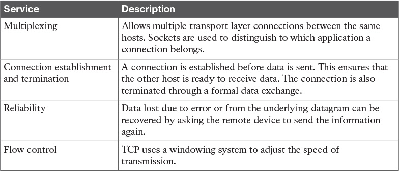
TCP Header
Application data is encapsulated in TCP segments by adding a TCP header to the application data. These segments are then passed to IP for further encapsulation, thus ensuring that the packets can be routed on the network, as shown on Figure 1-80.
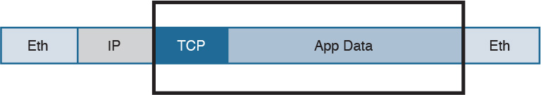
The TCP header is more extensive compared to the UDP header; this is because it needs additional fields to provide additional services and features. Figure 1-81 shows the TCP header structure.
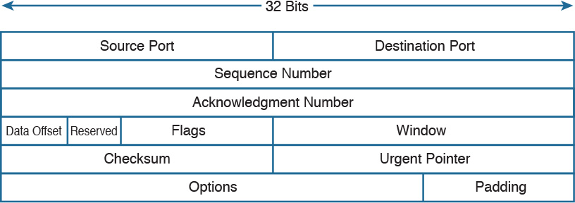
The main TCP header fields are as follows:
![]() Source and Destination Port: These are used to include the source and destination port for a given TCP packet. They are probably the most important fields within the TCP header and are used to correctly identify a TCP connection and TCP socket.
Source and Destination Port: These are used to include the source and destination port for a given TCP packet. They are probably the most important fields within the TCP header and are used to correctly identify a TCP connection and TCP socket.
![]() Sequence Number (32 bits): When the SYN flag bit is set to 1, this is the initial sequence number (ISN) and the first data byte is ISN+1. When the SYN flag bit is set to 0, this is the sequence number of the first data byte in this segment.
Sequence Number (32 bits): When the SYN flag bit is set to 1, this is the initial sequence number (ISN) and the first data byte is ISN+1. When the SYN flag bit is set to 0, this is the sequence number of the first data byte in this segment.
![]() Acknowledgment Number (32 bits): Once the connection is established, the ACK flag bit is set to 1, and the acknowledgment number provides the sequence number of the next data payload the sender of the packet is expecting to receive.
Acknowledgment Number (32 bits): Once the connection is established, the ACK flag bit is set to 1, and the acknowledgment number provides the sequence number of the next data payload the sender of the packet is expecting to receive.
![]() Control Flags (9 bits, 1 bit per flag): This field is used for congestion notification and to carry TCP flags.
Control Flags (9 bits, 1 bit per flag): This field is used for congestion notification and to carry TCP flags.
![]() ECN (Explicit Congestion Notification) Flags (3 bits): The first three flags (NS, CWR, ECE) are related to the congestion notification feature that has been recently defined in RFC 3168 and RFC 3540 (following RFC 793 about the TCP protocol in general). This feature supports end-to-end network congestion notification, in order to avoid dropping packets as a sign of network congestion.
ECN (Explicit Congestion Notification) Flags (3 bits): The first three flags (NS, CWR, ECE) are related to the congestion notification feature that has been recently defined in RFC 3168 and RFC 3540 (following RFC 793 about the TCP protocol in general). This feature supports end-to-end network congestion notification, in order to avoid dropping packets as a sign of network congestion.
![]() TCP flags include the following:
TCP flags include the following:
![]() URG: The Urgent flag signifies that Urgent Pointer data should be reviewed.
URG: The Urgent flag signifies that Urgent Pointer data should be reviewed.
![]() ACK: The Acknowledgment bit flag should be set to 1 after the connection has been established.
ACK: The Acknowledgment bit flag should be set to 1 after the connection has been established.
![]() PSH: The Push flag signifies that the data should be pushed directly to an application.
PSH: The Push flag signifies that the data should be pushed directly to an application.
![]() RST: The Reset flag resets the connection.
RST: The Reset flag resets the connection.
![]() SYN: The Synchronize (sequence numbers) flag is relevant for connection establishment, and should only be set within the first packets from both of the hosts.
SYN: The Synchronize (sequence numbers) flag is relevant for connection establishment, and should only be set within the first packets from both of the hosts.
![]() FIN: This flag signifies that there is no more data from sender.
FIN: This flag signifies that there is no more data from sender.
![]() Window (16 bits): This field indicates the number of data bytes the sender of the segment is able to receive. This field enables flow control.
Window (16 bits): This field indicates the number of data bytes the sender of the segment is able to receive. This field enables flow control.
![]() Urgent pointer (16 bits): When the URG flag is set to 1, this field indicates the sequence number of the data payload following the urgent data segment. The TCP protocol doesn’t define what the user will do with the urgent data; it only provides notification on urgent data pending processing.
Urgent pointer (16 bits): When the URG flag is set to 1, this field indicates the sequence number of the data payload following the urgent data segment. The TCP protocol doesn’t define what the user will do with the urgent data; it only provides notification on urgent data pending processing.
TCP Connection Establishment and Termination
As mentioned at the beginning of this section, the fact that the TCP protocol is connection oriented means that before any data is exchanged, the two hosts need to go through a process of establishing a connection. This process is often referred to as “three-way-handshake” because it involves three packets and the main goal is to synchronize the sequence numbers so that the hosts can exchange data, as illustrated in Figure 1-82.
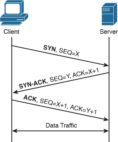
Let’s examine the packet exchange in more detail:
![]() First packet (SYN): The client starts the process of establishing a connection with a server by sending a TCP segment that has the SYN bit set to 1, in order to signal to the peer that it wants to synchronize the sequence numbers and establish the connection. The client also sends its initial sequence number (here X), which is a random number chosen by a client.
First packet (SYN): The client starts the process of establishing a connection with a server by sending a TCP segment that has the SYN bit set to 1, in order to signal to the peer that it wants to synchronize the sequence numbers and establish the connection. The client also sends its initial sequence number (here X), which is a random number chosen by a client.
![]() Second packet (SYN-ACK): The server responds with a SYN-ACK packet where it sends its own request for synchronization and its initial sequence number (another random number; here Y). Within the same packet, the server also sends the acknowledgment number X+1, acknowledging the receipt of a packet with the sequence number X and requesting the next packet with the sequence number X+1.
Second packet (SYN-ACK): The server responds with a SYN-ACK packet where it sends its own request for synchronization and its initial sequence number (another random number; here Y). Within the same packet, the server also sends the acknowledgment number X+1, acknowledging the receipt of a packet with the sequence number X and requesting the next packet with the sequence number X+1.
![]() Third packet (ACK): The client responds with a final acknowledgment, requesting the next packet with the sequence number Y+1.
Third packet (ACK): The client responds with a final acknowledgment, requesting the next packet with the sequence number Y+1.
In order to terminate a connection, peers go through a similar packet exchange, as shown in Figure 1-83.
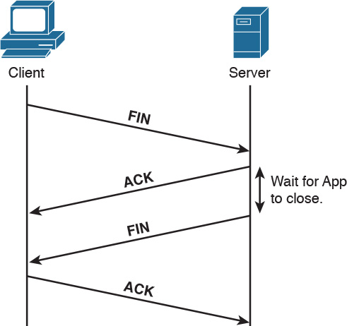
The process starts with the client’s application notifying the TCP layer on the client side that it wants to terminate the connection. The client sends a packet with the FIN bit set, to which the server responds with an acknowledgment, acknowledging the receipt of the packet. At that point, the server notifies the application on its side that the other peer wishes to terminate the connection. During this time, the client will still be able to receive traffic from the server, but will not be sending any traffic to the server. Once the application on the server side is ready to close down the connection, it signals to the TCP layer that the connection is ready to be closed, and the server sends a FIN packet as well, to which the client responds with an acknowledgment. At that point, the connection is terminated.
TCP Socket
The concept of multiplexing has already been introduced as a way to enable multiple applications to run on the same host and sockets by uniquely identifying a connection with an IP address, transport protocol, and port number.
There are some “well-known” applications that use designated port numbers (for example, WWW uses TCP port 80). This means that the web server will keep its socket for TCP port 80 open, listening to requests from various hosts. When a host tries to open a connection to a web server, it will use TCP port 80 as a destination port, and it will choose a random port number (greater than 1024) as a source port. Random port numbers need to be greater than 1024 because the ones up to 1024 are reserved for well-known applications.
Table 1-24 shows a list of some of the most used applications and their port numbers. A full list of ports used by known services can be found at http://www.iana.org/assignments/service-names-port-numbers/service-names-port-numbers.xhtml.
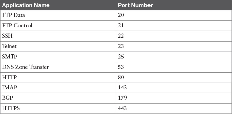
FTP (File Transfer Protocol) usesTCP port 20 for transferring the data and a separate connection on port 21 for exchanging control information (for example, FTP commands). Depending on whether the FTP server is in active or passive mode, different port numbers can be involved.
SSH (Secure Shell) is a protocol used for remote device management by allowing a secure (encrypted) connection over an unsecure medium. Telnet can also be used for device management; however, this is not recommended because FTP is not secure—data is sent in plaintext.
SMTP (Simple Mail Transfer Protocol) is used for email exchange. Typically, the client would use this protocol for sending emails, but would use POP3 or IMAP to retrieve emails from the mail server.
DNS (Domain Name System) uses UDP port 53 for domain name queries from hosts that allow other hosts to find out about the IP address for a specific domain name, but it uses TCP port 53 for communication between DNS servers for completing DNS zone transfers.
HTTP (Hypertext Transfer Protocol) is an application-based protocol that is used for accessing content on the Web. HTTPS (HTTP over Secure Socket Layer) is basically HTTP that uses TLS (Transport Layer Security) and SSL (Secure Sockets Layer) for encryption. HTTP is widely used on the Internet for secure communication because it allows encryption and server authentication.
BGP (Border Gateway Protocol) is an exterior gateway protocol used for exchanging routing information between different autonomous systems. It’s the routing protocol of the Internet.
TCP Error Detection and Recovery
TCP provides reliable delivery because the protocol is able to detect errors in transmission (for example, lost, damaged, or duplicated segments) and recover from such errors. This is done through the use of sequence numbers, acknowledgments, and checksum fields in the TCP header.
Each segment transmitted is marked with a sequence number, allowing the receiver of the segments to order them and provide acknowledgment on which segments have been received. If the sender doesn’t get acknowledgment, it will send the data again.
Figure 1-84 shows an example of sequence numbers and acknowledgments in a typical scenario.
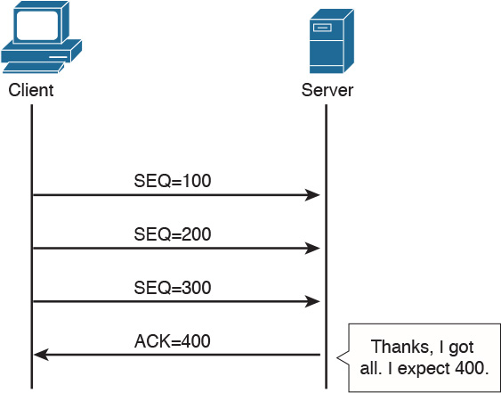
In this example, the client is sending three segments, each with 100 bytes of data. If the server has received all three segments in order, it would send a packet with the acknowledgment set to 400, which literally means “I’ve received all the segments with sequence numbers up to 399, and I am now expecting a segment with the sequence number 400.”
The fact that the segments have sequence numbers will allow the server to properly align the data upon receipt—for example, if for any reason it receives the segments in a different order or if it receives any duplicates.
Figure 1-85 shows how TCP detects and recovers from an error.
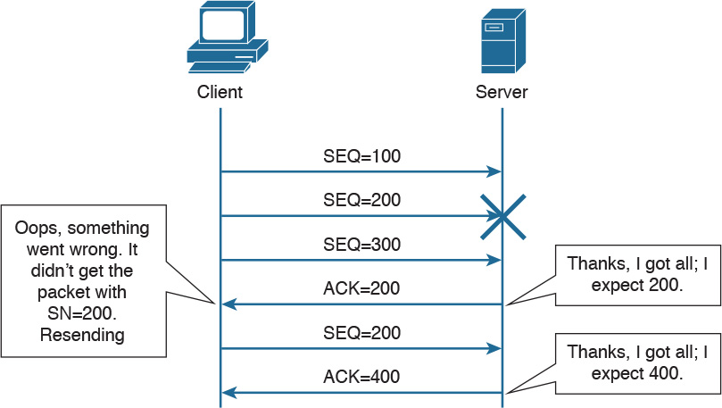
Imagine now that the client sends three packets with sequence numbers 100, 200, and 300. Due to some error in the transmission, the packet with the sequence number 200 gets lost or damaged. If the segment gets damaged during transmission, the TCP protocol would be able to detect this through the checksum number available within the TCP header. Because the packet with the sequence number 200 has not been received properly, the server will only send acknowledgement up to 200. This indicates to the client that it needs to resend that packet. When the server receives the missing packet, it will resume the normal acknowledge to 400, because it already received the packet with sequence numbers 300 and 400. This indicates to the client that it can send packets with sequence 500 and so on. It is worth mentioning that if the receiver doesn’t receive the packet with the sequence number 200, it will continue to send packets with acknowledgment number 200, asking for the missing packet.
TCP Flow Control
The TCP protocol ensures flow control through the use of “sliding windows,” by which a receiving host “tells” the sender how many bytes of data it can handle at a given time before waiting for an acknowledgment—this is called the window size. This mechanism works for both the client and server. For example, the client can ask the server to slow down, and the server can use this mechanism to ask the client to slow down or even to increase the speed. This allows the TCP peers to increase or reduce the speed of transmission depending on the conditions on the network and processing capability, and to avoid the situation of having a receiving host overwhelmed with data. The size of the receiving window is communicated through the “Window” field within the TCP header. Figure 1-86 shows how the window size gets adjusted based on the capability of the receiving host.
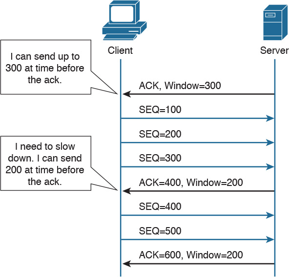
Initially, the server notifies the client that it can handle a window size of 300 bytes, so the client is able to send three segments of 100 bytes each, before getting the acknowledgment. However, if for some reason the server becomes overwhelmed with data that needs to be processed, it will notify the client that it can now handle a smaller window size.
The receiving host (for example, the server) has a certain buffer that it fills in with data received during a TCP connection, which could determine the size of this window. In ideal conditions, the receiving host may be able to process all the received data instantaneously, and free up the buffer again, leaving the window at the same size. However, if for some reason it is not able to process the data at that speed, it will reduce the window, which will notify the client of the problem. In Figure 1-86, the receiving party (the server) notifies the client that it needs to use a smaller window size of 200 bytes instead of the initial 300-byte window. The client adjusts its data stream accordingly. This process is dynamic, meaning that the server could also increase the window size.
The Window field in TCP header is 16 bits long, which means that the maximum window size is 65,535 bytes. In order to use higher window sizes, a scaling factor within the TCP Options field can be used. This TCP option will get negotiated within the initial three-way handshake.
User Datagram Protocol (UDP)
Like TCP, the User Datagram Protocol (UDP) is one of the most used transport layer protocols. Unlike TCP, however, UDP is designed to reduce the number of protocol iterations and complexity. It in fact does not establish any connection channel and in essence just wraps higher-layer information in a UDP segment and passes it to IP for transmission. UDP is usually referred as a “connectionless” protocol.
Due to its simplicity, UDP does not implement any mechanism for error control and retransmission; it leaves that task to the higher-layer protocols if required. Generally, UDP is used in applications where the low latency and low jitter are more important than reliability. A well-known use case for UDP is Voice over IP. UDP is described in RFC 768.
UDP Header
The UDP header structure is shorter and less complex than TCP’s. Figure 1-87 shows an example of a UDP header.
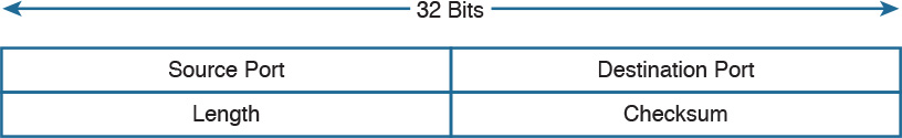
The UDP header includes the following fields:
![]() Source and Destination Port: Similar to the TCP header, these fields are used to determine the socket address and to correctly send the information to the higher-level application.
Source and Destination Port: Similar to the TCP header, these fields are used to determine the socket address and to correctly send the information to the higher-level application.
![]() Length: Includes the length of the UDP segment.
Length: Includes the length of the UDP segment.
![]() Checksum: It is built based on a pseudo header which includes information from the IP header (source and destination addresses) and information from the UDP header. Refer to the RFC for more information on how the checksum is calculated.
Checksum: It is built based on a pseudo header which includes information from the IP header (source and destination addresses) and information from the UDP header. Refer to the RFC for more information on how the checksum is calculated.
UDP Socket and Known UDP Application
As described earlier, UDP uses the same principle of multiplexing and sockets that’s used by TCP. The protocol information on the socket determines whether it is a TCP or UDP type of socket. As with TCP, UDP has well-known applications that use standard port numbers while listening for arriving packets. Table 1-25 provides an overview of known applications and their standard ports.
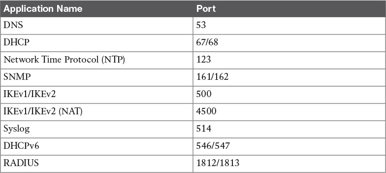
This concludes the overview of networking fundamentals. The next chapter introduces the concepts of network security devices and cloud services.
Exam Preparation Tasks
Review All Key Topics
Review the most important topics in the chapter, noted with the Key Topic icon in the outer margin of the page. Table 1-26 lists these key topics and the page numbers on which each is found.
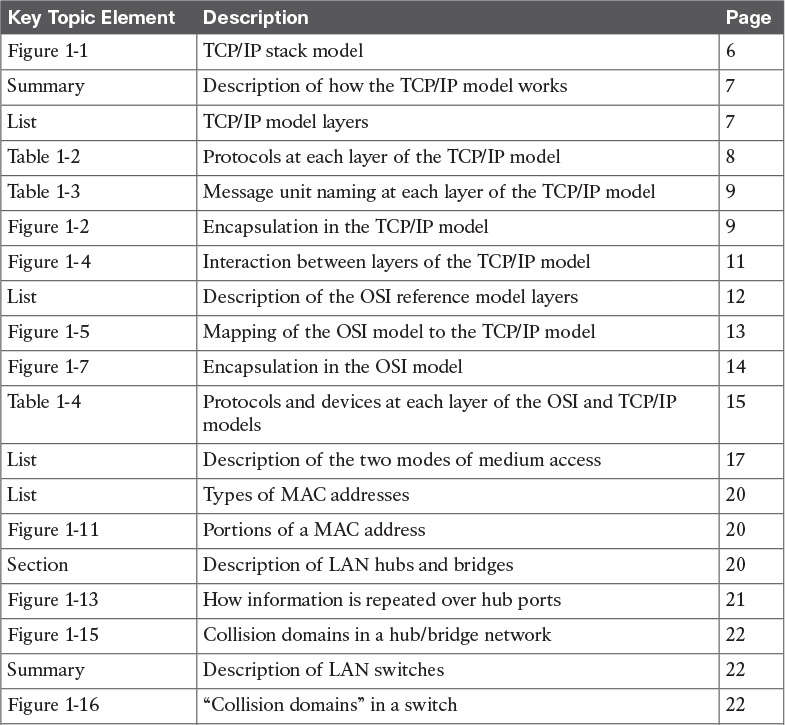
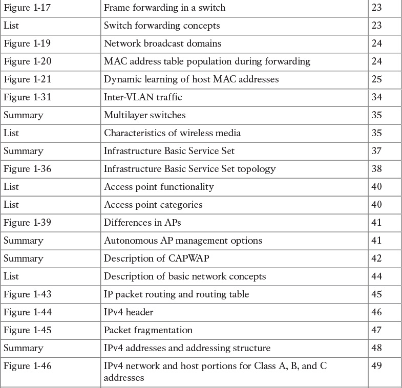
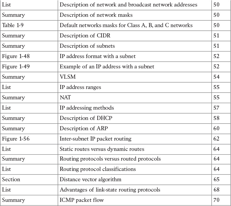
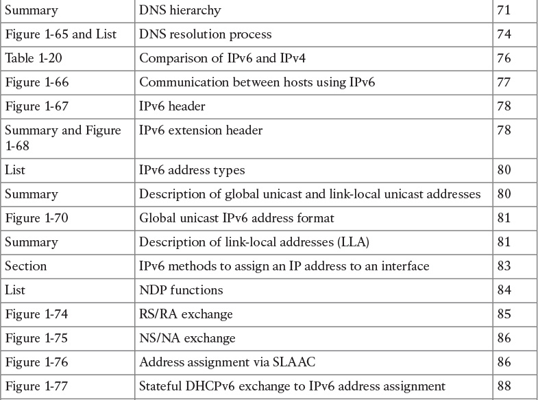
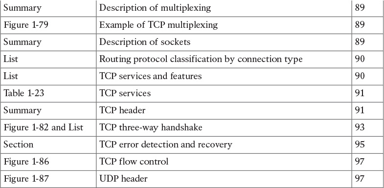
Complete Tables and Lists from Memory
Print a copy of Appendix B, “Memory Tables,” (found on the book website), or at least the section for this chapter, and complete the tables and lists from memory. Appendix C, “Memory Tables Answer Key,” also on the website, includes completed tables and lists to check your work.
Define Key Terms
Define the following key terms from this chapter, and check your answers in the glossary:
TCP/IP model
OSI model
local area network
Ethernet
collision domain
MAC address
LAN hub
LAN bridge
LAN switch
VLAN
trunk
wireless LAN
access point
lightweight access point
autonomous access point
Internet Protocol
private IP addresses
Classless Interdomain Routing (CIDR)
variable-length subnet Mask (VLSM)
Dynamic Host Configuration Protocol (DHCP)
Domain Name System
stateless address auto-configuration (SLAAC)
transport protocol socket
connectionless communication
connection-oriented communication
Q&A
The answers to these questions appear in Appendix A, “Answers to the ‘Do I Know This Already?’ Quizzes and Q&A Questions.” For more practice with exam format questions, use the exam engine on the website.
1. At which OSI layer does a router typically operate?
a. Transport
b. Network
c. Data link
d. Application
2. What are the advantages of a full-duplex transmission mode compared to half-duplex mode? (Select all that apply.)
a. Each station can transmit and receive at the same time.
b. It avoids collisions.
c. It makes use of backoff time.
d. It uses a collision avoidance algorithm to transmit.
3. How many broadcast domains are created if three hosts are connected to a Layer 2 switch in full-duplex mode?
a. 4
b. 3
c. None
d. 1
4. What is a trunk link used for?
a. To pass multiple virtual LANs
b. To connect more than two switches
c. To enable Spanning Tree Protocol
d. To encapsulate Layer 2 frames
5. What is the main difference between a Layer 2 switch and a multilayer switch?
a. A multilayer switch includes Layer 3 functionality.
b. A multilayer switch can be deployed on multiple racks.
c. A Layer 2 switch is faster.
d. A Layer 2 switch uses a MAC table whereas a multilayer switch uses an ARP table.
6. What is CAPWAP used for?
a. To enable wireless client mobility through different access points
b. For communication between a client wireless station and an access point
c. For communication between a lightweight access point and a wireless LAN controller
d. For communication between an access point and the distribution service
7. Which of the following services are provided by a lightweight access point? (Select all that apply.)
a. Channel encryption
b. Transmission and reception of frames
c. Client authentication
d. Quality of Service
8. Which of the following classful networks would allow at least 256 usable IPv4 addresses? (Select all that apply).
a. Class A
b. Class B
c. Class C
d. All of the above
9. What would be the maximum length of the network mask for a network that has four hosts?
a. /27
b. /30
c. /24
d. /29
10. Which routing protocol exchanges link state information?
a. RIPv2
b. RIP
c. OSPF
d. BGP
11. What is an advantage of using OSPF instead of RIPv2?
a. It does not have the problem of count to infinity.
b. OSPF has a higher hop-count value.
c. OSPF includes bandwidth information in the distance vector.
d. OSPF uses DUAL for optimal shortest path calculation.
12. What are two ways the IPv6 address 2345:0000:0000:0000:0000:0000:0100:1111 can be written?
a. 2345:0:0:0:0:0:0100:1111
b. 2345::1::1
c. 2345::0100:1111
d. 2345::1:1111
13. In IPv6, what is used to replace ARP?
a. ARPv6
b. DHCPv6
c. NDP
d. Route Advertisement Protocol
14. What would be the IPv6 address of a host using SLAAC with 2345::/64 as a network prefix and MAC address of 0300.1111.2222?
a. 2345::100:11FF:FE11:2222
b. 2345:0:0:0:0300:11FF:FE11:2222
c. 2345:0:0:0:FFFE:0300:1111:2222
d. 2345::0300:11FF:FE11:2222
15. What is a DNS iterative query used for?
a. It is sent from a DNS server to other servers to resolve a domain.
b. It is sent from a DNS resolver to the backup DNS server.
c. It is sent from a DNS server to the DNS client.
d. It is sent from a client machine to a DNS resolver.
16. Which TCP header flag is used by TCP to establish a connection?
a. URG
b. SYN
c. PSH
d. RST
17. What information is included in a network socket? (Select all that apply.)
a. Protocol
b. IP address
c. Port
d. MAC address
References and Further Reading
“Requirements for Internet Hosts – Communication Layers,” https://tools.ietf.org/html/rfc1122
ISO/IEC 7498-1 – Information technology – Open System Interconnection – Basic Reference Model: The Basic Model
David Hucaby, CCNA Wireless 200-355 Official Cert Guide, Cisco Press (2015)
DNS Best Practices, Network Protections, and Attack Identification
http://www.cisco.com/c/en/us/about/security-center/dns-best-practices.html
Wendell Odom, CCENT/CCNA ICND1 100-105 Official Cert Guide, Cisco Press (2016)
Wendell Odom, CCNA Routing and Switching ICND2 200-105 Official Cert Guide, Cisco Press (2016)
Cisco ICND1 Foundation Learning Guide: LANs and Ethernet
http://www.ciscopress.com/articles/article.asp?p=2092245&seqNum=2
IEEE Std 802.1D – IEEE Standard for Local and Metropolitan Area Networks – Media Access Control (MAC) Bridges
IEEE Std 802.1Q – IEEE Standard for Local and Metropolitan Area Networks – Bridges and Bridged Networks
IEEE Std 802 – IEEE Standard for Local and Metropolitan Area Networks: Overview and Architecture
“Address Allocation for Private Internets,” https://tools.ietf.org/html/rfc1918
“Special-Purpose IP Address Registries,” https://tools.ietf.org/html/rfc6890
“Dynamic Host Configuration Protocol,” https://www.ietf.org/rfc/rfc2131.txt
“An Ethernet Address Resolution Protocol,” https://tools.ietf.org/html/rfc826
“INTERNET CONTROL MESSAGE PROTOCOL,” https://tools.ietf.org/html/rfc792
“Domain Names - Implementation and Specification,” https://www.ietf.org/rfc/rfc1035.txt
“Internet Protocol, Version 6 (IPv6),” Specification https://tools.ietf.org/html/rfc2460
“Unique Local IPv6 Unicast Addresses,” https://tools.ietf.org/html/rfc4193
“IP Version 6 Addressing Architecture,” https://tools.ietf.org/html/rfc4291
“IPv6 Secure Neighbor Discovery,” http://www.cisco.com/en/US/docs/ios-xml/ios/sec_data_acl/configuration/15-2mt/ip6-send.html
“Privacy Extensions for Stateless Address Autoconfiguration in IPv6,” https://tools.ietf.org/html/rfc4941
“SEcure Neighbor Discovery (SEND),” https://tools.ietf.org/html/rfc3971
“Cryptographically Generated Addresses (CGA),” https://tools.ietf.org/html/rfc3972
“IPv6 Stateless Address Autoconfiguration,” https://tools.ietf.org/search/rfc4862
“Transmission Control Protocol,” https://tools.ietf.org/html/rfc793
“User Datagram Protocol,” https://tools.ietf.org/html/rfc768