
3
Filters and transforms
The various chapters of this book concentrate on some specific subjects, but in all of these some common principles or processes arise. The most important of these is filtering, and its parallel topic of transforms. Filters and transforms are inseparable from this technology. They are relevant to sampling, displays, recording, transmission and compression systems.
3.1 Introduction
In convergent systems it is very important to remember that the valuable commodity is information. For practical reasons the way information is represented may have to be changed a number of times during its journey. If accuracy or realism is a goal these changes must be well engineered. In the course of this book we shall explore changes between the continuous domain of real sounds and images and the discrete domain of sampled data. A proper understanding of these processes requires familiarity with the principles of filters and transforms, which is why this chapter precedes the treatment of conversion in Chapter 4.
Figure 3.1 shows an optical system of finite resolution. If an object containing an infinitely sharp line is presented to this system, the image will be an intensity function known in optics as a point spread function. Such functions are almost invariably symmetrical in optics. There is no movement or change here, the phenomenon is purely spatial. A point spread function is a spatial impulse response. All images passing through the optical system are convolved with it.
Figure 3.1(b) shows that the object may be scanned by an analog system to produce a waveform. The image may also be scanned in this way.
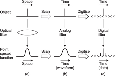
Figure 3.1 In optical systems an infinitely sharp line is reproduced as a point spread function (a) which is the impulse response of the optical path. Scanning either object or image produces an analog time-variant waveform (b). The scanned object waveform can be converted to the scanned image waveform with an electrical filter having an impulse response which is an analog of the point spread function. (c) The object and image may also be sampled or the object samples can be converted to the image samples by a filter with an analogous discrete impulse response.
These waveforms are now temporal. However, the second waveform may be obtained in another way, using an analog filter in series with the first scanned waveform which has an equivalent impulse response. This filter must have linear phase, i.e. its impulse response must be symmetrical.
Figure 3.1(c) shows that the object may also be sampled in which case all samples but one will have a value of zero. The image may also be sampled, and owing to the point spread function, there will now be a number of non-zero sample values. However, the image samples may also be obtained by passing the input sample into a digital filter having the appropriate impulse response. Note that it is possible to obtain the same result as (c) by passing the scanned waveform of (b) into an ADC and storing the samples in a memory.
Clearly there are a number of equivalent routes leading to the same result. One result of this is that optical systems and sampled systems can simulate one another. This gives us considerable freedom to perform processing in the most advantageous domain which gives the required result. There are many parallels between analog, digital and optical filters, which this chapter treats as a common subject.
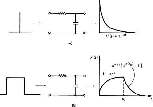
It should be clear from Figure 3.1 why video signal paths need to have linear phase. In general, analog circuitry and filters tend not to have linear phase because they must be causal, which means that the output can only occur after the input. Figure 3.2(a) shows a simple RC network and its impulse response. This is the familiar exponential decay due to the capacitor discharging through the resistor (in series with the source impedance which is assumed here to be negligible). The figure also shows the response to a squarewave at (b). With other waveforms the process is inevitably more complex.
Filtering is unavoidable. Sometimes a process has a filtering effect which is undesirable, for example the limited frequency response of an audio amplifier or loss of resolution in a lens, and we try to minimize it. On other occasions a filtering effect is specifically required. Analog or digital filters, and sometimes both, are required in ADCs, DACs, in the data channels of digital recorders and transmission systems and in DSP. Optical filters may also be necessary in imaging systems to convert between sampled and continuous images. Optical systems used in displays and in laser recorders also act as spatial filters.1
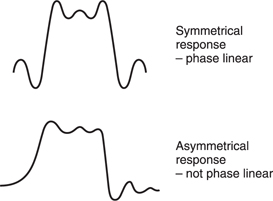
Figure 3.3 shows that impulse response testing tells a great deal about a filter. In a perfect filter, all frequencies should experience the same time delay. If some groups of frequencies experience a different delay than others, there is a group-delay error. As an impulse contains an infinite spectrum, a filter suffering from group-delay error will separate the different frequencies of an impulse along the time axis.
A pure delay will cause a phase shift proportional to frequency, and a filter with this characteristic is said to be phase-linear. The impulse response of a phase-linear filter is symmetrical. If a filter suffers from group-delay error it cannot be phase-linear. It is almost impossible to make a perfectly phase-linear analog filter, and many filters have a groupdelay equalization stage following them which is often as complex as the filter itself. In the digital domain it is straightforward to make a phaselinear filter, and phase equalization becomes unnecessary.
Because of the sampled nature of the signal, whatever the response at low frequencies may be, all PCM channels (and sampled analog channels) act as low-pass filters because they cannot contain frequencies above the Nyquist limit of half the sampling frequency.
3.2 Transforms
Transforms are a useful subject because they can help to understand processes which cause undesirable filtering or to design filters. The information itself may be subject to a transform. Transforming converts the information into another analog. The information is still there, but expressed with respect to temporal or spatial frequency rather than time or space. Instead of binary numbers representing the magnitude of samples, there are binary numbers representing the magnitude of frequency coefficients. The close relationship of transforms to convergent technologies makes any description somewhat circular as Figure 3.4 shows. The solution adopted in this chapter is to introduce a number of filtering-related topics, and to return to the subject of transforms whenever a point can be illustrated.
Transforms are only a different representation of the same information. As a result what happens in the frequency domain must always be consistent with what happens in the time or space domains. A filter may modify the frequency response of a system, and/or the phase response, but every combination of frequency and phase response has a corresponding impulse response in the time domain.
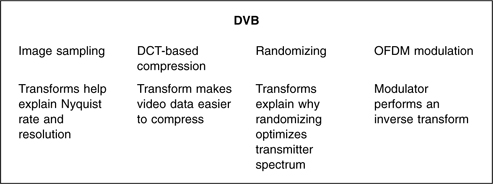
Figure 3.5 shows the relationship between the domains. On the left is the frequency domain. Here an input signal having a given spectrum is input to a filter having a given frequency response. The output spectrum will be the product of the two functions. If the functions are expressed logarithmically in deciBels, the product can be obtained by simple addition.
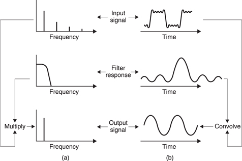
Figure 3.5 If a signal having a given spectrum is passed into a filter, multiplying the two spectra will give the output spectrum at (a). Equally transforming the filter frequency response will yield the impulse response of the filter. If this is convolved with the time domain waveform, the result will be the output waveform, whose transform is the output spectrum (b).
On the right, the time-domain output waveform represents the convolution of the impulse response with the input waveform. However, if the frequency transform of the output waveform is taken, it must be the same as the result obtained from the frequency response and the input spectrum. This is a useful result because it means that when image or audio sampling is considered, it will be possible to explain the process in both domains.
3.3 Convolution
When a waveform is input to a system, the output waveform will be the convolution of the input waveform and the impulse response of the system. Convolution can be followed by reference to a graphic example in Figure 3.6. Where the impulse response is asymmetrical, the decaying tail occurs after the input. As a result it is necessary to reverse the impulse response in time so that it is mirrored prior to sweeping it through the input waveform. The output voltage is proportional to the shaded area shown where the two impulses overlap. If the impulse response is symmetrical, as would be the case with a linear phase filter, or in an optical system, the mirroring process is superfluous.
The same process can be performed in the sampled, or discrete time domain as shown in Figure 3.7. The impulse and the input are now a set of discrete samples which clearly must have the same sample spacing. The impulse response only has value where impulses coincide. Elsewhere it is zero. The impulse response is therefore stepped through the input one sample period at a time. At each step, the area is still proportional to the output, but as the time steps are of uniform width, the area is proportional to the impulse height and so the output is obtained by adding up the lengths of overlap. In mathematical terms, the output samples represent the convolution of the input and the impulse response by summing the coincident cross-products.
3.4 FIR and IIR filters
Filters can be described in two main classes, as shown in Figure 3.8, according to the nature of the impulse response. Finite-impulse response (FIR) filters are always stable and, as their name suggests, respond to an impulse once, as they have only a forward path. In the temporal domain, the time for which the filter responds to an input is finite, fixed and readily established. The same is therefore true about the distance over which a FIR filter responds in the spatial domain. FIR filters can be made perfectly phase-linear if a significant processing delay is accepted. Most filters used for image processing, sampling rate conversion and oversampling fall into this category.
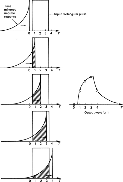
Figure 3.6 In the convolution of two continuous signals (the impulse response with the input), the impulse must be time reversed or mirrored. This is necessary because the impulse will be moved from left to right, and mirroring gives the impulse the correct time-domain response when it is moved past a fixed point. As the impulse response slides continuously through the input waveform, the area where the two overlap determines the instantaneous output amplitude. This is shown for five different times by the crosses on the output waveform.
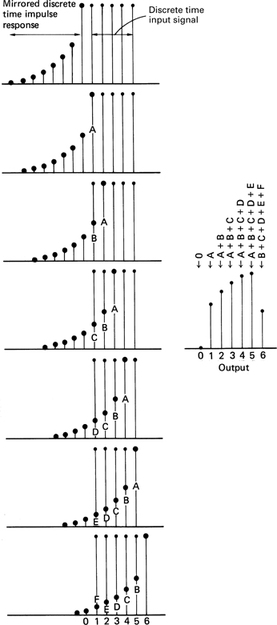
Figure 3.7 In discrete time convolution, the mirrored impulse response is stepped through the input one sample period at a time. At each step, the sum of the cross-products is used to form an output value. As the input in this example is a constant height pulse, the output is simply proportional to the sum of the coincident impulse response samples. This figure should be compared with Figure 3.6.
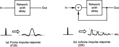
Infinite-impulse response (IIR) filters respond to an impulse indefinitely and are not necessarily stable, as they have a return path from the output to the input. For this reason they are also called recursive filters. As the impulse response is not symmetrical, IIR filters are not phaselinear. Audio equalizers often employ recursive filters.
3.5 FIR filters
A FIR filter performs convolution of the input waveform with its own impulse response. It does this by graphically constructing the impulse response for every input sample and superimposing all these responses. It is first necessary to establish the correct impulse response. Figure 3.9(a) shows an example of a low-pass filter which cuts off at 1/4 of the sampling rate. The impulse response of an ideal low-pass filter is a sinx/x curve, where the time between the two central zero crossings is the reciprocal of the cut-off frequency. According to the mathematics, the waveform has always existed, and carries on for ever.
The peak value of the output coincides with the input impulse. This means that the filter cannot be causal, because the output has changed before the input is known. Thus in all practical applications it is necessary to truncate the extreme ends of the impulse response, which causes an aperture effect, and to introduce a time delay in the filter equal to half the duration of the truncated impulse in order to make the filter causal. As an input impulse is shifted through the series of registers in Figure 3.9(b), the impulse response is created, because at each point it is multiplied by a coefficient as in (c).
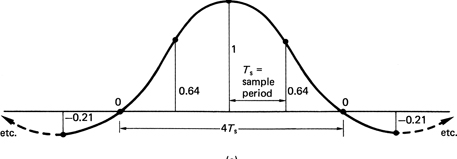
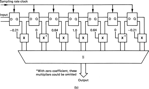
Figure 3.9(b) The structure of an FIR LPF. Input samples shift across the register and ateach point are multiplied by different coefficients.
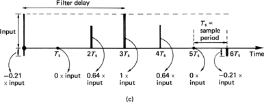
Figure 3.9(c) When a single unit sample shifts across the circuit of Figure 3.9(b), the impulse response is created at the output as the impulse is multiplied by each coefficient in turn.
These coefficients are simply the result of sampling and quantizing the desired impulse response. Clearly the sampling rate used to sample the impulse must be the same as the sampling rate for which the filter is being designed. In practice the coefficients are calculated, rather than attempting to sample an actual impulse response. The coefficient wordlength will be a compromise between cost and performance. Because the input sample shifts across the system registers to create the shape of the impulse response, the configuration is also known as a transversal filter. In operation with real sample streams, there will be several consecutive sample values in the filter registers at any time in order to convolve the input with the impulse response.
Simply truncating the impulse response causes an abrupt transition from input samples which matter and those which do not. Truncating the filter superimposes a rectangular shape on the time-domain impulse response. In the frequency domain the rectangular shape transforms to a sinx/x characteristic which is superimposed on the desired frequency response as a ripple. One consequence of this is known as Gibb’s phenomenon; a tendency for the response to peak just before the cut-off frequency.2,3 As a result, the length of the impulse which must be considered will depend not only on the frequency response, but also on the amount of ripple which can be tolerated. If the relevant period of the impulse is measured in sample periods, the result will be the number of points or multiplications needed in the filter. Figure 3.10 compares the performance of filters with different numbers of points. A high-quality digital audio FIR filter may need in excess of 100 points.
Rather than simply truncate the impulse response in time, it is better to make a smooth transition from samples which do not count to those that do. This can be done by multiplying the coefficients in the filter by a window function which peaks in the centre of the impulse. Figure 3.11 shows some different window functions and their responses. The rectangular window is the case of truncation, and the response is shown at I. A linear reduction in weight from the centre of the window to the edges characterizes the Bartlett window II, which trades ripple for an increase in transition-region width. At III is shown the Hann window, which is essentially a raised cosine shape. Not shown is the similar Hamming window, which offers a slightly different trade-off between ripple and the width of the main lobe. The Blackman window introduces an extra cosine term into the Hamming window at half the period of the main cosine period, reducing Gibb’s phenomenon and ripple level, but increasing the width of the transition region. The Kaiser window is a family of windows based on the Bessel function, allowing various tradeoffs between ripple ratio and main lobe width. Two of these are shown in IV and V.
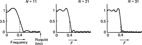
Figure 3.10 The truncation of the impulse in an FIR filter caused by the use of a finite number of points (N) results in ripple in the response. Shown here are three different numbers of points for the same impulse response. The filter is an LPF which rolls off at 0.4 of the fundamental interval. (Courtesy Philips Technical Review.)
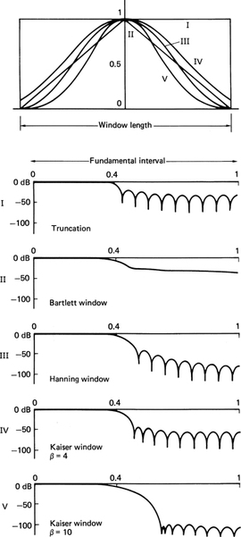
Figure 3.11 The effect of window functions. At top, various window functions are shown in continuous form. Once the number of samples in the window is established, the continuous functions shown here are sampled at the appropriate spacing to obtain window coefficients. These are multiplied by the truncated impulse response coefficients to obtain the actual coefficients used by the filter. The amplitude responses I–V correspond to the window functions illustrated. (Responses courtesy Philips Technical Review.)
The Dolph window4 shown in Figure 3.12 results in an equiripple filter which has the advantage that the attenuation in the stopband never falls below a certain level.
Filter coefficients can be optimized by computer simulation. One of the best-known techniques used is the Remez exchange algorithm, which converges on the optimum coefficients after a number of iterations.
In the example of Figure 3.13, a low-pass FIR filter is shown which is intended to allow downsampling by a factor of two. The key feature is that the stopband must have begun before one half of the output sampling rate. This is most readily achieved using a Hamming window because it was designed empirically to have a flat stopband so that good aliasing attenuation is possible. The width of the transition band determines the number of significant sample periods embraced by the impulse. The Hamming window doubles the width of the transition band. This determines in turn both the number of points in the filter, and the filter delay. For the purposes of illustration, the number of points is much smaller than would normally be the case in an audio application.
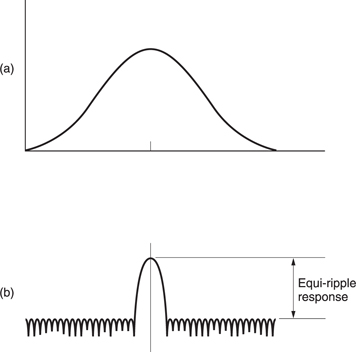
Figure 3.12 The Dolph window shape is shown at (a). The frequency response is at (b). Note the constant height of the response ripples.
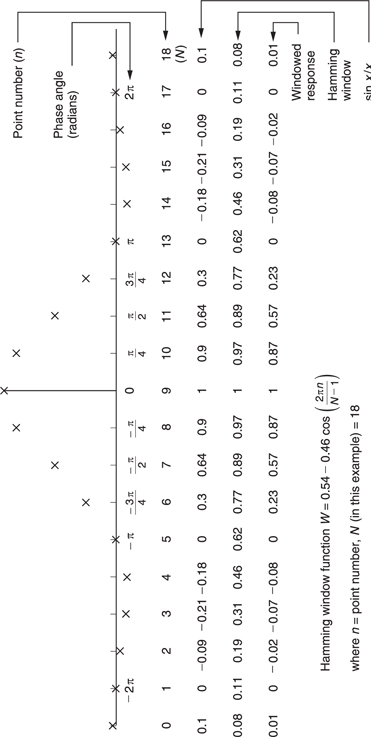
As the impulse is symmetrical, the delay will be half the impulse period. The impulse response is a sinx/x function, and this has been calculated in the figure. The equation for the Hamming window function is shown with the window values which result. The sinx/x response is next multiplied by the Hamming window function to give the windowed impulse response shown.
If the coefficients are not quantized finely enough, it will be as if they had been calculated inaccurately, and the performance of the filter will be less than expected. Figure 3.14 shows an example of quantizing coefficients. Conversely, raising the wordlength of the coefficients increases cost.
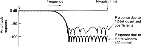
Figure 3.14 Frequency response of a 49-point transversal filter with infinite precision (solid line) shows ripple due to finite window size. Quantizing coefficients to twelve bits reduces attenuation in the stopband. (Responses courtesy Philips Technical Review.)
The FIR structure is inherently phase-linear because it is easy to make the impulse response absolutely symmetrical. The individual samples in a digital system do not know in isolation what frequency they represent, and they can only pass through the filter at a rate determined by the clock. Because of this inherent phase-linearity, a FIR filter can be designed for a specific impulse response, and the frequency response will follow.
The frequency response of the filter can be changed at will by changing the coefficients. A programmable filter only requires a series of PROMs to supply the coefficients; the address supplied to the PROMs will select the response. The frequency response of a digital filter will also change if the clock rate is changed, so it is often less ambiguous to specify a frequency of interest in a digital filter in terms of a fraction of the fundamental interval rather than in absolute terms. The configuration shown in Figure 3.9 serves to illustrate the principle. The units used on the diagrams are sample periods and the response is proportional to these periods or spacings, and so it is not necessary to use actual figures.
Where the impulse response is symmetrical, it is often possible to reduce the number of multiplications, because the same product can be used twice, at equal distances before and after the centre of the window. This is known as folding the filter. A folded filter is shown in Figure 3.15.
3.6 Sampling-rate conversion
Sampling-rate conversion or interpolation is an important enabling technology on which a large number of practical digital video devices are based. In digital video, the sampling rate takes on many guises. When analog video is sampled in real time, the sampling rate is temporal, but where pixels form a static array, the sampling rate is a spatial frequency.
Some of the applications of interpolation are set out below:
1 Video standards convertors need to change two of the sampling rates of the signal they handle, namely the temporal frame rate and the vertical line spacing, which is in fact a spatial sampling frequency. In some lowbit rate video applications such as Internet video, the frame rate may deliberately be reduced. The display will have to increase it again to avoid flicker.
2 In digital audio, different sampling rates exist today for different purposes. Rate conversion allows material to be exchanged freely between such formats.
3 To take advantage of oversampling convertors, an increase in sampling rate is necessary for DACs and a reduction in sampling rate is necessary for ADCs. In oversampling the factors by which the rates are changed are simpler than in other applications.
4 In image processing, a large number of different standard pixel array sizes exists. Changing between these formats may be necessary in order to view an incoming image on an available display. This technique is generally known as resizing and is essentially a two-dimensional sampling rate conversion. The rate in this case is the spatial frequency of the pixels.
5 Rate conversion allows interchange of real-time PCM data between systems whose sampling clocks are not synchronized.
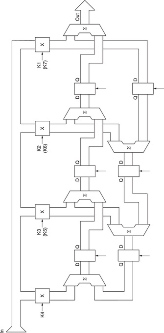
Figure 3.15 A seven-point folded filter for a symmetrical impulse response. In this case K1 and K7 will be identical, and so the input sample can be multiplied once, and the product fed into the output shift system in two different places. The centre coefficient K4 appears once. In an even-numbered filter the centre coefficient would also be used twice.
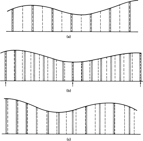
Figure 3.16 Categories of rate conversion. (a) Integer-ratio conversion, where the lower-rate samples are always coincident with those of the higher rate. There are a small number of phases needed. (b) Fractional-ratio conversion, where sample coincidence is periodic. A larger number of phases is required. Example here is conversion from 50.4 kHz to 44.1 kHz (8/7). (c) Variable-ratio conversion, where there is no fixed relationship, and a large number of phases are required.
There are three basic but related categories of rate conversion, as shown in Figure 3.16. The most straightforward (a) changes the rate by an integer ratio, up or down. The timing of the system is thus simplified because all samples (input and output) are present on edges of the higher-rate sampling clock. Such a system is generally adopted for oversampling convertors; the exact sampling rate immediately adjacent to the analog domain is not critical, and will be chosen to make the filters easier to implement.
Next in order of difficulty is the category shown at (b) where the rate is changed by the ratio of two small integers. Samples in the input periodically time-align with the output. Such devices can be used for converting between the various rates of ITU-601.
The most complex rate-conversion category is where there is no simple relationship between input and output sampling rates, and in fact they may vary. This situation shown at (c), is known as variable-ratio conversion. The temporal or spatial relationship of input and output samples is arbitrary. This problem will be met in effects machines which zoom or rotate images.
The technique of integer-ratio conversion is used in conjunction with oversampling convertors in digital video and audio and in motion estimation and compression systems where sub-sampled or reduced resolution versions of an input image are required. These applications will be detailed in Chapter 5.
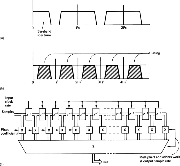
Figure 3.17 The spectrum of a typical digital sample stream at (a) will be subject to aliasing as in (b) if the baseband width is not reduced by an LPF. At (c) an FIR low-pass filter prevents aliasing. Samples are clocked transversely across the filter at the input rate, but the filter only computes at the output sample rate. Clearly this will only work if the two are related by an integer factor.
Figure 3.17(a) shows the spectrum of a typical sampled system where the sampling rate is a little more than twice the analog bandwidth. Attempts to reduce the sampling rate by simply omitting samples, a process known as decimation, will result in aliasing, as shown in Figure 3.17(b). Intuitively it is obvious that omitting samples is the same as if the original sampling rate was lower. In order to prevent aliasing, it is necessary to incorporate low-pass filtering into the system where the cutoff frequency reflects the new, lower, sampling rate. An FIR type low-pass filter could be installed, as described earlier in this chapter, immediately prior to the stage where samples are omitted, but this would be wasteful, because for much of its time the FIR filter would be calculating sample values which are to be discarded. The more effective method is to combine the low-pass filter with the decimator so that the filter only calculates values to be retained in the output sample stream. Figure 3.17(c) shows how this is done. The filter makes one accumulation for every output sample, but that accumulation is the result of multiplying all relevant input samples in the filter window by an appropriate coefficient. The number of points in the filter is determined by the number of input samples in the period of the filter window, but the number of multiplications per second is obtained by multiplying that figure by the output rate. If the filter is not integrated with the decimator, the number of points has to be multiplied by the input rate. The larger the rate-reduction factor, the more advantageous the decimating filter ought to be, but this is not quite the case, as the greater the reduction in rate, the longer the filter window will need to be to accommodate the broader impulse response.
When the sampling rate is to be increased by an integer factor, additional samples must be created at even spacing between the existing ones. There is no need for the bandwidth of the input samples to be reduced since, if the original sampling rate was adequate, a higher one must also be adequate.
Figure 3.18 shows that the process of sampling-rate increase can be thought of in two stages. First, the correct rate is achieved by inserting samples of zero value at the correct instant, and then the additional samples are given meaningful values by passing the sample stream through a low-pass filter which cuts off at the Nyquist frequency of the original sampling rate. This filter is known as an interpolator, and one of its tasks is to prevent images of the lower input-sampling spectrum from appearing in the extended baseband of the higher-rate output spectrum.
All sampled systems have finite bandwidth and need a reconstruction filter to remove the frequencies above the baseband due to sampling.
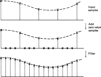
Figure 3.18 In integer-ratio sampling, rate increase can be obtained in two stages. First, zero-value samples are inserted to increase the rate, and then filtering is used to give the extra samples real values. The filter necessary will be an LPF with a response which cuts off at the Nyquist frequency of the input samples.
After reconstruction, one infinitely short digital sample ideally represents a sinx/x pulse whose central peak width is determined by the response of the reconstruction filter, and whose amplitude is proportional to the sample value. This implies that, in reality, one sample value has meaning over a considerable timespan, rather than just at the sample instant. This will be detailed in Chapter 4. Were this not true, it would be impossible to build an interpolator.
Performing the steps of rate increase separately is inefficient. The bandwidth of the information is unchanged when the sampling rate is increased; therefore the original input samples will pass through the filter unchanged, and it is superfluous to compute them. The combination of the two processes into an interpolating filter minimizes the amount of computation.
As the purpose of the system is purely to increase the sampling rate, the filter must be as transparent as possible, and this implies that a linearphase configuration is mandatory, suggesting the use of an FIR structure. Figure 3.19 shows that the theoretical impulse response of such a filter is a sinx/x curve which has zero value at the position of adjacent input samples. In practice this impulse cannot be implemented because it is infinite. The impulse response used will be truncated and windowed as described earlier. To simplify this discussion, assume that a sinx/x impulse is to be used. There is a strong parallel with the operation of a DAC where the analog voltage is returned to the time-continuous state by summing the analog impulses due to each sample. In a digital interpolating filter, this process is duplicated.5
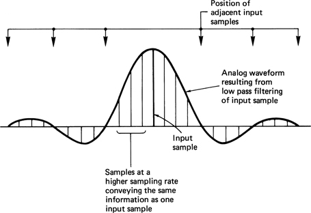
Figure 3.19 A single sample results in a sinx/x waveform after filtering in the analog domain. At a new, higher, sampling rate, the same waveform after filtering will be obtained if the numerous samples of differing size shown here are used. It follows that the values of these new samples can be calculated from the input samples in the digital domain in an FIR filter.
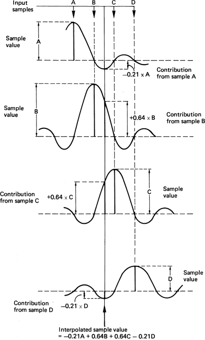
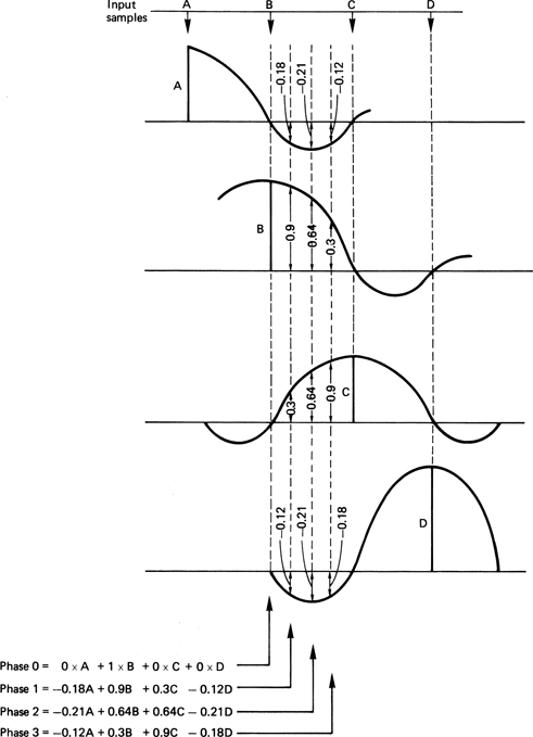
If the sampling rate is to be doubled, new samples must be interpolated exactly halfway between existing samples. The necessary impulse response is shown in Figure 3.20; it can be sampled at the output sample period and quantized to form coefficients. If a single input sample is multiplied by each of these coefficients in turn, the impulse response of that sample at the new sampling rate will be obtained. Note that every other coefficient is zero, which confirms that no computation is necessary on the existing samples; they are just transferred to the output. The intermediate sample is computed by adding together the impulse responses of every input sample in the window. The figure shows how this mechanism operates. If the sampling rate is to be increased by a factor of four, three sample values must be interpolated between existing input samples. Figure 3.21 shows that it is only necessary to sample the impulse response at one-quarter the period of input samples to obtain three sets of coefficients which will be used in turn. In hardwareimplemented filters, the input sample which is passed straight to the output is transferred by using a fourth filter phase where all coefficients are zero except the central one which is unity.
Fractional ratio conversion allows interchange between different images having different pixel array sizes. Fractional ratios also occur in the vertical axis of standards convertors. Figure 3.16 showed that when the two sampling rates have a simple fractional relationship m/n, there is a periodicity in the relationship between samples in the two streams. It is possible to have a system clock running at the least-common multiple frequency which will divide by different integers to give each sampling rate.6
The existence of a common clock frequency means that a fractional-ratio convertor could be made by arranging two integer-ratio converters in series. This configuration is shown in Figure 3.22(a). The input-sampling rate is multiplied by m in an interpolator, and the result is divided by n in a decimator. Although this system would work, it would be grossly inefficient, because only one in n of the interpolator’s outputs would be used. A decimator followed by an interpolator would also offer the correct sampling rate at the output, but the intermediate sampling rate would be so low that the system bandwidth would be quite unacceptable.
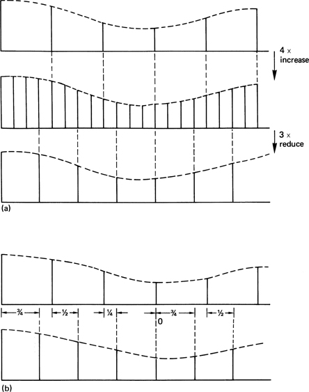
Figure 3.22 At (a), fractional-ratio conversion of 3/4 in this example is by increasing to 4× input prior to reducing by 3×. The inefficiency due to discarding previously computed values is clear. At (b), efficiency is raised since only needed values will be computed. Note how the interpolation phase changes for each output. Fixed coefficients can no longer be used.
As has been seen, a more efficient structure results from combining the processes. The result is exactly the same structure as an integer-ratio interpolator, and requires an FIR filter. The impulse response of the filter is determined by the lower of the two sampling rates, and, as before, it prevents aliasing when the rate is being reduced, and prevents images when the rate is being increased. The interpolator has sufficient coefficient phases to interpolate m output samples for every input sample, but not all of these values are computed; only interpolations which coincide with an output sample are performed. It will be seen in Figure 3.22(b) that input samples shift across the transversal filter at the input sampling rate, but interpolations are only performed at the output sample rate. This is possible because a different filter phase will be used at each interpolation.
In the previous examples, the sample rate or spacing of the filter output had a constant relationship to the input, which meant that the two rates had to be phase-locked. This is an undesirable constraint in some applications, including image manipulators. In a variable-ratio interpolator, values will exist for the points at which input samples were made, but it is necessary to compute what the sample values would have been at absolutely any point between available samples. The general concept of the interpolator is the same as for the fractional-ratio convertor, except that an infinite number of filter phases is ideally necessary. Since a realizable filter will have a finite number of phases, it is necessary to study the degradation this causes. The desired continuous temporal or spatial axis of the interpolator is quantized by the phase spacing, and a sample value needed at a particular point will be replaced by a value for the nearest available filter phase. The number of phases in the filter therefore determines the accuracy of the interpolation. The effects of calculating a value for the wrong point are identical to those of sampling with clock jitter, in that an error occurs proportional to the slope of the signal. The result is program-modulated noise. The higher the noise specification, the greater the desired time accuracy and the greater the number of phases required. The number of phases is equal to the number of sets of coefficients available, and should not be confused with the number of points in the filter, which is equal to the number of coefficients in a set (and the number of multiplications needed to calculate one output value).
The sampling jitter accuracy necessary for eight-bit working is measured in picoseconds. This implies that something like 32 filter phases will be required for adequate performance in an eight-bit sampling-rate convertor.
3.7 Transforms and duality
The duality of transforms provides an interesting insight into what is happening in common processes. Fourier analysis holds that any periodic waveform can be reproduced by adding together an arbitrary number of harmonically related sinusoids of various amplitudes and phases. Figure 3.23 shows how a square wave can be built up of harmonics. The spectrum can be drawn by plotting the amplitude of the harmonics against frequency. It will be seen that this gives a spectrum which is a decaying wave. It passes through zero at all even multiples of the fundamental. The shape of the spectrum is a sinx/x curve. If a square wave has a sinx/x spectrum, it follows that a filter with a rectangular impulse response will have a sinx/x spectrum.
A low-pass filter has a rectangular spectrum, and this has a sinx/x impulse response. These characteristics are known as a transform pair. In transform pairs, if one domain has one shape of the pair, the other domain will have the other shape. Figure 3.24 shows a number of transform pairs.
At (a) a squarewave has a sinx/x spectrum and a sinx/x impulse has a square spectrum. In general the product of equivalent parameters on either side of a transform remains constant, so that if one increases, the other must fall. If (a) shows a filter with a wider bandwidth, having a narrow impulse response, then (b) shows a filter of narrower bandwidth which has a wide impulse response. This is duality in action. The limiting case of this behaviour is where one parameter becomes zero, the other goes to infinity. At (c) a time-domain pulse of infinitely short duration has a flat spectrum. Thus a flat waveform, i.e. DC, has only zero in its spectrum. The impulse response of the optics of a laser disk (d) has a sin2x/x2 intensity function, and this is responsible for the triangular falling frequency response of the pickup. The lens is a rectangular aperture, but as there is no such thing as negative light, a sinx/x impulse response is impossible. The squaring process is consistent with a positiveonly impulse response. Interestingly the transform of a Gaussian response in still Gaussian.
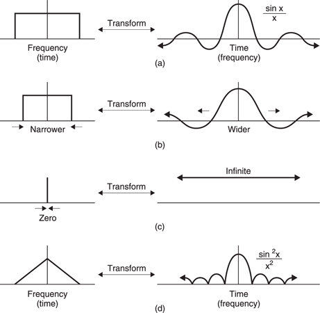
Figure 3.24 Transform pairs. At (a) the dual of a rectangle is a sinx/x function. If one is time domain, the other is frequency domain. At (b), narrowing one domain widens the other. The limiting case of this is (c). Transform of the sinx/x squared function is triangular.
Duality also holds for sampled systems. A sampling process is periodic in the time domain. This results in a spectrum which is periodic in the frequency domain. If the time between the samples is reduced, the bandwidth of the system rises. Figure 3.25(a) shows that a continuous time signal has a continuous spectrum whereas at (b) the frequency transform of a sampled signal is also discrete. In other words sampled signals can only be analysed into a finite number of frequencies. The more accurate the frequency analysis has to be, the more samples are needed in the block. Making the block longer reduces the ability to locate a transient in time. This is the Heisenberg inequality which is the limiting case of duality, because when infinite accuracy is achieved in one domain, there is no accuracy at all in the other.
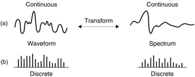
Figure 3.25 Continuous time signal (a) has continuous spectrum. Discrete time signal (b) has discrete spectrum.
3.8 The Fourier transform
Figure 3.23 showed that if the amplitude and phase of each frequency component is known, linearly adding the resultant components in an inverse transform results in the original waveform. In digital systems the waveform is expressed as a number of discrete samples. As a result the Fourier transform analyses the signal into an equal number of discrete frequencies. This is known as a discrete Fourier transform or DFT in which the number of frequency coefficients is equal to the number of input samples. The fast Fourier transform is no more than an efficient way of computing the DFT.7 As was seen in the previous section, practical systems must use windowing to create short-term transforms.
It will be evident from Figure 3.26 that the knowledge of the phase of the frequency component is vital, as changing the phase of any component will seriously alter the reconstructed waveform. Thus the DFT must accurately analyse the phase of the signal components.
There are a number of ways of expressing phase. Figure 3.27 shows a point which is rotating about a fixed axis at constant speed. Looked at from the side, the point oscillates up and down at constant frequency. The waveform of that motion is a sine wave, and that is what we would see if the rotating point were to translate along its axis whilst we continued to look from the side.
One way of defining the phase of a waveform is to specify the angle through which the point has rotated at time zero (T = 0). If a second point is made to revolve at 90° to the first, it would produce a cosine wave when translated. It is possible to produce a waveform having arbitrary phase by adding together the sine and cosine waves in various proportions and polarities. For example, adding the sine and cosine waves in equal proportions results in a waveform lagging the sine wave by 45°.
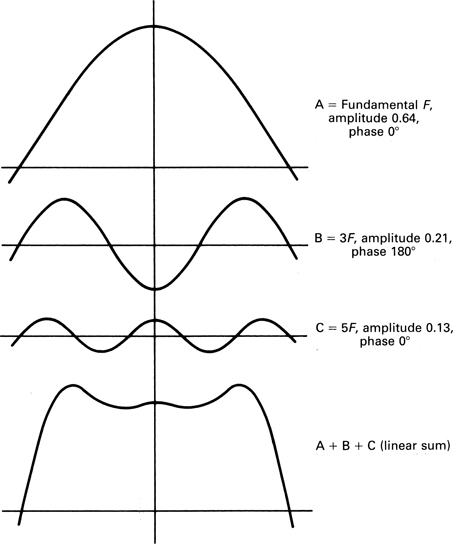
Figure 3.27 shows that the proportions necessary are respectively the sine and the cosine of the phase angle. Thus the two methods of describing phase can be readily interchanged.
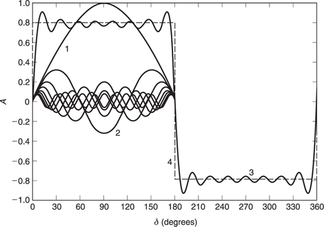
The discrete Fourier transform spectrum-analyses a string of samples by searching separately for each discrete target frequency. It does this by multiplying the input waveform by a sine wave, known as the basis function, having the target frequency and adding up or integrating the products. Figure 3.28(a) shows that multiplying by basis functions gives a non-zero integral when the input frequency is the same, whereas (b) shows that with a different input frequency (in fact all other different frequencies) the integral is zero showing that no component of the target frequency exists. Thus from a real waveform containing many frequencies all frequencies except the target frequency are excluded. The magnitude of the integral is proportional to the amplitude of the target component.
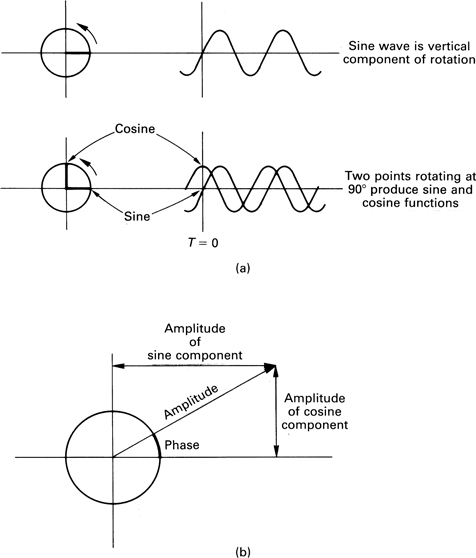
Figure 3.28(c) shows that the target frequency will not be detected if it is phase shifted 90° as the product of quadrature waveforms is always zero. Thus the discrete Fourier transform must make a further search for the target frequency using a cosine basis function. It follows from the arguments above that the relative proportions of the sine and cosine integrals reveal the phase of the input component. Thus each discrete frequency in the spectrum must be the result of a pair of quadrature searches.
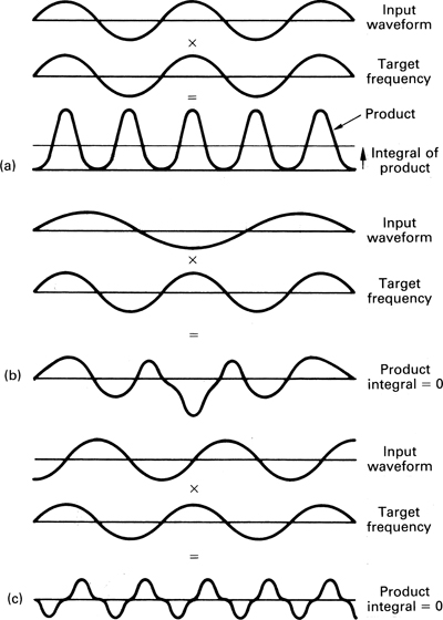
Figure 3.28 The input waveform is multiplied by the target frequency and the result is averaged or integrated. At (a) the target frequency is present and a large integral results. With another input frequency the integral is zero as at (b). The correct frequency will also result in a zero integral shown at (c) if it is at 90° to the phase of the search frequency. This is overcome by making two searches in quadrature.
Searching for one frequency at a time as above will result in a DFT, but only after considerable computation. However, a lot of the calculations are repeated many times over in different searches. The fast Fourier transform gives the same result with less computation by logically gathering together all the places where the same calculation is needed and making the calculation once.
The amount of computation can be reduced by performing the sine and cosine component searches together. Another saving is obtained by noting that every 180° the sine and cosine have the same magnitude but are simply inverted in sign. Instead of performing four multiplications on two samples 180° apart and adding the pairs of products it is more economical to subtract the sample values and multiply twice, once by a sine value and once by a cosine value.
The first coefficient is the arithmetic mean which is the sum of all the sample values in the block divided by the number of samples. Figure 3.29 shows how the search for the lowest frequency in a block is performed. Pairs of samples are subtracted as shown, and each difference is then multiplied by the sine and the cosine of the search frequency. The process shifts one sample period, and a new sample pair is subtracted and multiplied by new sine and cosine factors. This is repeated until all the sample pairs have been multiplied. The sine and cosine products are then added to give the value of the sine and cosine coefficients respectively.
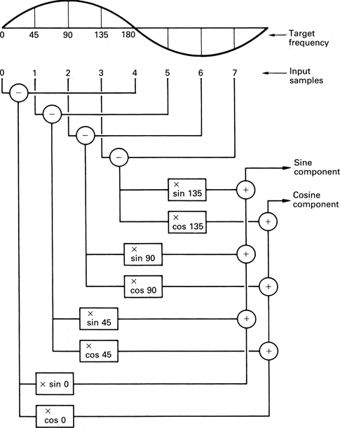
Figure 3.29 An example of a filtering search. Pairs of samples are subtracted and multiplied by sampled sine and cosine waves. The products are added to give the sine and cosine components of the search frequency.
It is possible to combine the calculation of the DC component which requires the sum of samples and the calculation of the fundamental which requires sample differences by combining stages shown in Figure 3.30(a) which take a pair of samples and add and subtract them. Such a stage is called a butterfly because of the shape of the schematic. Figure 3.30(b) shows how the first two components are calculated. The phase rotation boxes attribute the input to the sine or cosine component outputs according to the phase angle. As shown, the box labelled 90° attributes nothing to the sine output, but unity gain to the cosine output. The 45° box attributes the input equally to both components.
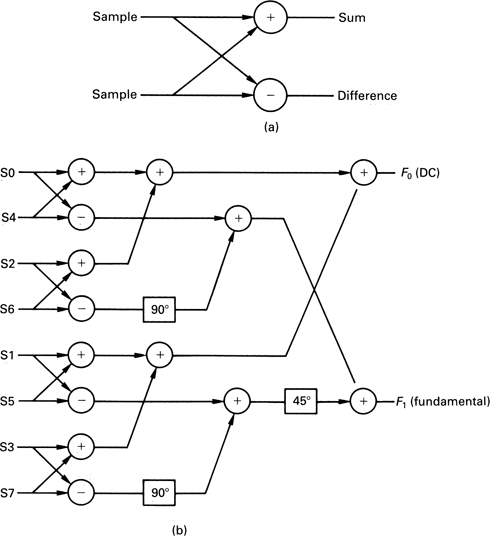
Figure 3.30 The basic element of an FFT is known as a butterfly as at (a) because of the shape of the signal paths in a sum and difference system. The use of butterflies to compute the first two coefficients is shown in (b).
Figure 3.30(c) shows a numerical example. If a sinewave input is considered where zero degrees coincides with the first sample, this will produce a zero sine coefficient and non-zero cosine coefficient. Figure 3.30(d) shows the same input waveform shifted by 90°. Note how the coefficients change over.
Figure 3.30(e) shows how the next frequency coefficient is computed. Note that exactly the same first-stage butterfly outputs are used, reducing the computation needed.
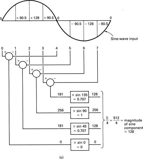
Figure 3.30(c) An actual calculation of a sine coefficient. This should be compared with the result shown in (d).
A similar process may be followed to obtain the sine and cosine coefficients of the remaining frequencies. The full FFT diagram for eight samples is shown in Figure 3.31(a). The spectrum this calculates is shown in (b). Note that only half of the coefficients are useful in a real bandlimited system because the remaining coefficients represent frequencies above one half of the sampling rate.
In STFTs the overlapping input sample blocks must be multiplied by window functions. The principle is the same as for the application in FIR filters shown in section 3.5. Figure 3.32 shows that multiplying the search frequency by the window has exactly the same result except that this need be done only once and much computation is saved. Thus in the STFT the basis function is a windowed sine or cosine wave.
The FFT is used extensively in such applications as phase correlation, where the accuracy with which the phase of signal components can be analysed is essential. It also forms the foundation of the discrete cosine transform.
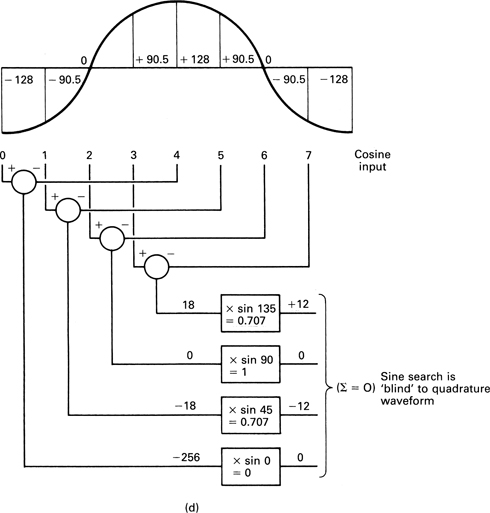
Figure 3.30(d) With a quadrature input the frequency is not seen.
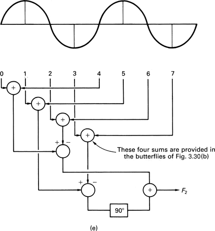
Figure 3.30(e) The butterflies used for the first coefficients form the basis of the computation of the next coefficient.
3.9 The discrete cosine transform (DCT)
The DCT is a special case of a discrete Fourier transform in which the sine components of the coefficients have been eliminated leaving a single number. This is actually quite easy. Figure 3.33(a) shows a block of input samples to a transform process. By repeating the samples in a timereversed order and performing a discrete Fourier transform on the double-length sample set a DCT is obtained. The effect of mirroring the input waveform is to turn it into an even function whose sine coefficients are all zero. The result can be understood by considering the effect of individually transforming the input block and the reversed block.
Figure 3.33(b) shows that the phase of all the components of one block are in the opposite sense to those in the other. This means that when the components are added to give the transform of the double length block all the sine components cancel out, leaving only the cosine coefficients, hence the name of the transform.8 In practice the sine component calculation is eliminated. Another advantage is that doubling the block length by mirroring doubles the frequency resolution, so that twice as many useful coefficients are produced. In fact a DCT produces as many useful coefficients as input samples.
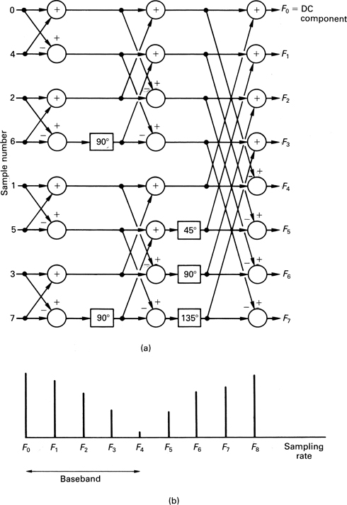
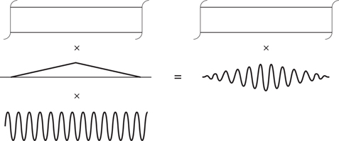
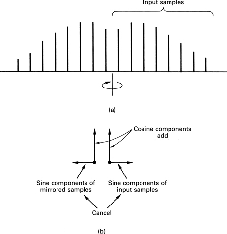
Figure 3.33 The DCT is obtained by mirroring the input block as shown at (a) prior to an FFT. The mirroring cancels out the sine components as at (b), leaving only cosine coefficients.
For image processing two-dimensional transforms are needed. In this case for every horizontal frequency, a search is made for all possible vertical frequencies. A two-dimensional DCT is shown in Figure 3.34. The DCT is separable in that the two-dimensional DCT can be obtained by computing in each dimension separately. Fast DCT algorithms are available.9
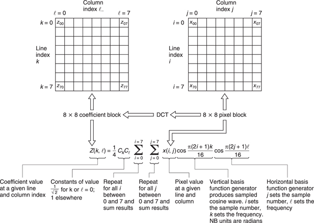
Figure 3.35 shows how a two-dimensional DCT is calculated by multiplying each pixel in the input block by terms which represent sampled cosine waves of various spatial frequencies. A given DCT coefficient is obtained when the result of multiplying every input pixel in the block is summed. Although most compression systems, including JPEG and MPEG, use square DCT blocks, this is not a necessity and rectangular DCT blocks are possible and are used in, for example, the DV format.
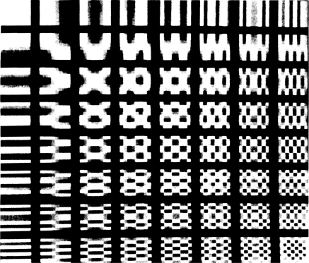
Figure 3.34 The discrete cosine transform breaks up an image area into discrete frequencies in two dimensions. The lowest frequency can be seen here at the top left corner. Horizontal frequency increases to the right and vertical frequency increases downwards.
The DCT is primarily used in MPEG-2 because it converts the input waveform into a form where redundancy can be easily detected and removed. More details of the DCT can be found in Chapter 9.
3.10 The wavelet transform
The wavelet transform was not discovered by any one individual, but has evolved via a number of similar ideas and was only given a strong mathematical foundation relatively recently.10–13 The wavelet transform is similar to the Fourier transform in that it has basis functions of various frequencies which are multiplied by the input waveform to identify the frequencies it contains. However, the Fourier transform is based on periodic signals and endless basis functions and requires windowing. The wavelet transform is fundamentally windowed, as the basis functions employed are not endless sine waves, but are finite on the time axis; hence the name. Wavelet transforms do not use a fixed window, but instead the window period is inversely proportional to the frequency being analysed. As a result a useful combination of time and frequency resolutions is obtained. High frequencies corresponding to transients in audio or edges in video are transformed with short basis functions and therefore are accurately located. Low frequencies are transformed with long basis functions which have good frequency resolution.
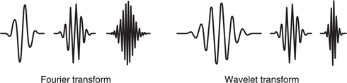
Figure 3.36 shows that that a set of wavelets or basis functions can be obtained simply by scaling (stretching or shrinking) a single wavelet on the time axis. Each wavelet contains the same number of cycles such that as the frequency reduces the wavelet gets longer. Thus the frequency discrimination of the wavelet transform is a constant fraction of the signal frequency. In a filter bank such a characteristic would be described as ‘constant Q’. Figure 3.37 shows that the division of the frequency domain by a wavelet transform is logarithmic whereas in the Fourier transform the division is uniform. The logarithmic coverage is effectively dividing the frequency domain into octaves and as such parallels the frequency discrimination of human hearing.
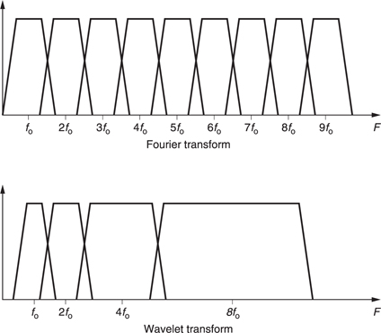
Figure 3.37 Wavelet transforms divide the frequency domain into octaves instead of the equal bands of the Fourier transform.
References
1.Ray, S.F., Applied Photographic Optics, Oxford: Focal Press (1988) (Ch. 17)
2.van den Enden, A.W.M. and Verhoeckx, N.A.M., Digital signal processing: theoretical background. Philips Tech. Rev., 42, 110–144, (1985)
3.McClellan, J.H., Parks, T.W. and Rabiner, L.R., A computer program for designing optimum FIR linear-phase digital filters. IEEE Trans. Audio and Electroacoustics, AU-21, 506–526 (1973)
4.Dolph, C.L., A current distribution for broadside arrays which optimises the relationship between beam width and side-lobe level. Proc. IRE, 34, 335–348 (1946)
5.Crochiere, R.E. and Rabiner, L.R., Interpolation and decimation of digital signals – a tutorial review. Proc. IEEE, 69, 300–331 (1981)
6.Rabiner, L.R., Digital techniques for changing the sampling rate of a signal. In B. Blesser, B. Locanthi and T.G. Stockham Jr (eds), Digital Audio, pp. 79–89, New York: Audio Engineering Society (1982)
7.Kraniauskas, P., Transforms in Signals and Systems, Chapter 6. Wokingham: Addison- Wesley (1992)
8.Ahmed, N., Natarajan, T. and Rao, K., Discrete Cosine Transform, IEEE Trans. Computers, C-23, 90–93 (1974)
9.De With, P.H.N., Data compression techniques for digital video recording, Ph.D thesis, Technical University of Delft (1992)
10. Goupillaud, P., Grossman, A. and Morlet, J., Cycle-Octave and related transforms in seismic signal analysis. Geoexploration, 23, 85–102, Elsevier Science (1984/5)
11. Daubechies, I., The wavelet transform, time–frequency localisation and signal analysis. IEEE Trans. Info. Theory, 36, No.5, 961–1005 (1990)
12. Rioul, O. and Vetterli, M., Wavelets and signal processing. IEEE Signal Process. Mag., 14–38 (Oct. 1991)
13. Strang, G. and Nguyen, T., Wavelets and Filter Banks, Wellesly, MA: Wellesley– Cambridge Press (1996)