
CHAPTER 4
Despill
When an object is filmed in front of a greenscreen, green light from the brightly lit green backing screen contaminates the foreground object in a variety of ways. The edges of the foreground object are not perfectly sharp due to lens limitations, so the edges become blended with the green backing. There may also be semi-transparent elements, such as smoke or glass, and the ever-present wisps of hair. There can be shiny elements that reflect the green backing regardless of how much dulling spray is used. Then there is the ubiquitous flare and spill.
Flare is seen as a green “haze” that covers everything in the frame, including the foreground object you are trying to isolate from the green backing. It is caused by the flood of green light entering the camera and bouncing around inside, lightly exposing the negative all over to green. The second contamination is spill. This stems from the fact that the green backing is in fact emitting a great deal of green light, some of which shines directly on areas of the foreground object that are visible to the camera.
The example in Color Plate 38 shows a close-up of a greenscreen and some blonde hair. The next example, Color Plate 39, reveals the contamination that the greenscreen left on the foreground layer when it was composited over a neutral gray background without any spill removal. All of this contamination must be removed for the composite to look right, and the despill operation does this job. This chapter explains how despill operations work, and, equally important, how they introduce artifacts. In addition to understanding the inner operations of the despill nodes in your software, you will also see how to “roll your own” despill operations in the event that you don't have any, or to solve special problems, which you are sure to have. Again, throughout this chapter we will be using the greenscreen to represent bluescreen as well.
The despill process is another example of a cheat that is not mathematically valid. A theoretically correct despill process would require a great deal of separate information about every object in the scene and the light sources shining on them— a totally impractical prospect. What we do have is a few simple techniques that work fairly well under most circumstances and introduce serious artifacts under some circumstances.
Even the very powerful off-the-shelf keyers such as Ultimatte will sometimes introduce despill artifacts. Even though they have very sophisticated algorithms that have been tested and refined over many years, they can still have problems. Your only recourse in this situation is to have as many despill methodologies as possible at your disposal so that you can switch algorithms to find one that does not introduce artifacts with your particular scene content.
4.1 The Despill Operation
In broad strokes, the despill operation simply removes the excess green from the greenscreen plate based on some rule, from which there are many to choose. The de-spilled version of the greenscreen is then used as the foreground layer of the composite.
The sequence of operations can be seen starting with the original greenscreen plate in Color Plate 44. After the despill operation in Color Plate 45, the green backing has been suppressed to a dark gray and the green flare has been removed. The despilled version is then used as the foreground layer in the final composite shown in Color Plate 46. A simplified flowgraph of the entire sequence of operations is illustrated in Figure 4-1. The greenscreen layer (labeled as “GS” in the flowgraph) is split into two branches. One branch is used to pull the matte and the other is de-spilled for the composite.
There are three ways the despill operation might be introduced to the composite. With an off-the-shelf keyer the despill operation as well as the matte extraction operations are internal to the keyer. The artist will be able to adjust the despill parameters to tweak it. The problem with this arrangement is that the despilled foreground layer will invariably need color correcting, and the keyer may not offer this option. You really don't want to color correct the greenscreen before it goes into the keyer because it will seriously disturb both the matte extraction and despill operations. The second way to add the despill operation to the composite is if your software has a despill node. The third way is to develop your own despill operations with discrete nodes, which we will be discussing in detail.
4.2 Despill Artifacts
The despill is done with some rule, and this despill rule can be very simple or very complex. The best rule is not necessarily the most complex. The best rule is the one that gives the best results with the fewest artifacts. The problem is that the rule that removes the spill is necessarily much more simple-minded than the rules of optics that created spill in the first place. As a result, any simple spill removal rule will be wrong everywhere in the plate to some degree. Depending on the scene content, it may be only a little bit wrong everywhere, so the results are quite acceptable. In other cases it can be seriously wrong in key areas and introduce such severe artifacts that something must be done.
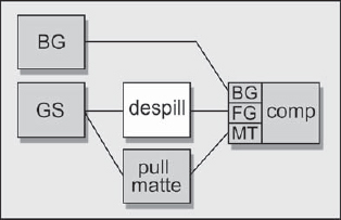
Figure 4-1: Flowgraph of the Composite with Despill Operation
There are primarily two color-related despill artifacts: hue shifts and brightness drops. The hue shift is caused by the fact that only one color channel, the green channel, is being modified, and changing one value in any RGB color triplet will cause a hue shift. Sometimes the hue shift is so visually slight as to go unnoticed. Other times the amount of green removed relative to the other two channels is enough to dramatically shift the hue, ruining the shot. The brightness drop comes from the fact that for greenscreens it is green that is being removed, and green is the majority component of the eye's perception of brightness. When the green is removed from around the edge, so is some brightness. In this regard bluescreens may have a slight advantage because blue is the lowest contributor to the eye's perception of brightness, so dropping the blue channel will not cause the apparent drop in brightness that green does.
Another artifact that despill operations can introduce with film elements is increased graininess. The blue channel of film is much grainier than the red or green channels, and this extra graininess even survives the telecine transfer to video. Some despill algorithms will use this grainy blue channel as a limiter for the green. As a result, the blue grain can become “embossed” on the green channel, adding an appalling, blotchy chatter to skin tones. There are solutions to this problem, of course, but it requires the artist who would fix it to understand what causes it in the first place. Since this is a film chemistry problem, if the scene was captured in video to begin with there is no blue grain bias.
4.3 Despill Algorithms
The problem with despill operations is that colorspace is vast and the despill operation is a simple image processing trick. This means that no single despill algorithm can solve all problems. If you are using the despill operation within a keyer, you normally cannot change the despill algorithm. All you can do is tweak the settings. This will sometimes fail to fix the problem, and heroic measures will be required. This section describes a variety of different despill algorithms but, perhaps more important, it also lays the foundations for you to develop custom solutions to custom problems.
4.3.1 Green Limited by Red
This is the simplest of all possible despill algorithms and yet it is surprising how often it gives satisfactory results. The rule is simply “limit the green channel to be no greater than the red channel.” Simply put, for each pixel, if the green channel is greater than the red channel, clip it to be equal to the red channel. If it is less than or equal to the red channel, then leave it alone.
Figure 4-2 illustrates a slice graph of just the red and green channels of a section of a greenscreen plate that spans a transition between a foreground (FG) object and the greenscreen (GS) green backing region (the blue channel is not involved in this case). In the foreground region the red channel is greater than the green channel, as we might expect for a skin tone, for example; the green channel becomes dominant as the graph transitions into the green backing region. The results of the “green limited by red” despill operation can be seen in Figure 4-3. Everywhere that the green channel was greater than the red channel it was clipped to be equal to the red channel (the green line is drawn above the red line for clarity—they would actually have the same values).
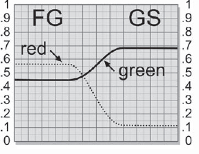
Figure 4-2: Original Greenscreen Plate
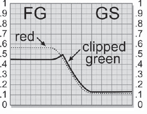
Figure 4-3: Despilled Greenscreen Plate
A real-world example of a despill operation in action can be seen starting with Color Plate 40, which adds a slice line crossing from the greenscreen backing well into the blonde hair. The resulting slice graph in Color Plate 41 shows all three color records and how the green channel is the dominant color even well into the hair. Of course, this is what we expected based on the green spill example from Color Plate 39. After the despill operation, however, the hair in Color Plate 42 is free of the excess green, and its slice graph in Color Plate 43 shows how the green channel is now “trimmed” to the level of the red channel. In those locations where the green channel was already less than the red channel it was unaffected. The despilled green channel is drawn just underneath the red channel for comparison. In actuality it would lie right on top of it, covering it up except where it actually drops below it.
4.3.1.1 Implementing the Algorithm
There are two ways you could implement this despill algorithm in your software. You can use a channel arithmetic node or build it out of simple discrete math operation nodes. If you have a channel math node and are friends with it, the equation would look like this:
Despilled green = if G > R then R: else G(Eq. 4-1)
which reads “if green is greater than red then use red: else use green.” The red and blue channels are left untouched. It simply substitutes the red pixel value for the green if it finds that the green pixel value is greater. Of course, you will have to translate this equation into the specific syntax of your particular channel math node.
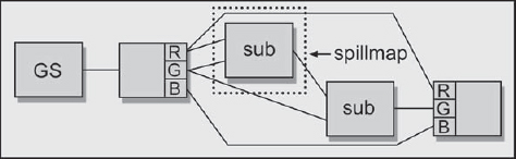
Figure 4-4: Despill Flowgraph: Green Limited by Red
Some of you may not have a channel math node, or may not like using it if you do. Fine. The equivalent process can be done with a couple of subtract nodes instead. Because flowgraph nodes don't support logic tests such as “if/then,” the discrete node approach requires a few more steps.
Figure 4-4 shows the flowgraph setup for this despill operation. Starting at the left, the greenscreen (GS) plate goes to a channel splitter. The first subtract (sub) node subtracts G – R, creating the spillmap—a channel that contains all of the green spill, any green that exceeds the red. More on this spillmap in a moment. The next subtract node subtracts this spillmap from the original green channel. This removes all of the excess green from the original green channel, clipping it to be equal to the red channel. The output of this subtract node is the despilled green channel. The last node merely recombines the despilled green channel with the original red and blue channels to create the final despilled greenscreen plate, then off you go to color correct and composite.
4.3.1.2 The Spillmap
The spillmap is a monochrome image that contains all of the excess green from the original greenscreen plate. Simply subtracting the spillmap from the green channel will produce the despilled image. In fact, the various despill methods really boil down to different ways of generating the spillmap. Once you have a map of all of the excess green in a spillmap, however it is created, you have the key to a despill operation. Of course, those folks who elect to use the channel math node or a keyer do not generate a separate spillmap, and in that regard they are at a bit of a disadvantage. There are several very cool things that you can do with a spillmap, which will be explored a bit later.
The slice graph in Figure 4-5 shows the transition from the skin tones of the subject to the green backing region. The shaded region shows the excess green that will be lifted out and placed into the spillmap from the G – R subtraction operation. In the FG region the skin tones are red dominant, so there is no excess green. As a result, the spillmap will have zero black in this region. When this part of the spillmap is subtracted from the skin it will not remove any green. In the greenscreen backing region (GS) the green channel is much larger than the red, so the results of the G – R subtraction produce a large residue of excess green for the spillmap.
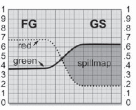
Figure 4-5: Slice Graph of the Spillmap Region
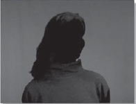
Figure 4-6: Spillmap from Greenscreen in Color Plate 1
Figure 4-6 shows the actual spillmap for the despilled greenscreen Color Plate 45. As expected, the green backing area has a great deal of excess green. However, there is something else. It also shows some excess green in the hair and on the sweater. Green spill in the hair we can do without, so removing this will be an improvement. But what about the sweater? It also showed up in the spillmap even though it is not part of the green spill we are trying to fix. It showed up simply because it is a light yellow with its green channel greater than its red channel. Unfortunately, when this spillmap is subtracted from the original greenscreen plate the sweater color will also loose some green, resulting in a hue shift toward orange which you can easily see by comparing Color Plate 44 and Color Plate 45. This is exactly the kind of artifact described earlier in Section 4.2, “Despill Artifacts.”
Whether or not this is a serious problem that has to be fixed totally depends on the circumstances. This could be just an actress in a scene and the color of her sweater doesn't really matter, or it might be a sweater commercial and the color of the sweater is the entire point of the spot. If it has to be fixed, there are two approaches. One is to mask off the afflicted region and protect it from the despill operation. The second approach is to select a different despill equation that does not disturb the sweater. Of course, it may disturb something else, but that something else may be totally acceptable. Inspecting the spillmap to find where the non-zero pixels are will reveal what parts of the picture are going to be affected by the despill operation.
The spillmap slice graph in Figure 4-5 reveals another artifact of despill operations that you should be aware of. In the middle third of the slice graph you can see the entire transition region where the FG blends into the GS part of the graph. The spillmap, however, starts near the middle of that transition region where the red and green channels actually cross. To be totally correct, it should start at the beginning of the transition region, further to the left. In other words, the spillmap does not penetrate far enough into the true edge of the transition region. In some other part of the picture the spillmap will penetrate deeper, and in other parts much less deeply. This means that the excess green will be removed from only the outermost edges of the foreground region, and how “outer” that is will change around the perimeter of the foreground object based on the local RGB values. This is usually not a noticeable problem, but occasionally it will be, so it is important to have alternatives at your disposal.
4.3.2 Green Limited by Blue
This, of course, is identical to the green limited by red process—it simply substitutes the blue channel for the red channel as the green limiter. For use in a channel math node the equation becomes:
Despilled green = if G > B then B: else G(Eq. 4-2)
When implemented with discrete nodes in a flowgraph (Figure 4-4), it is simply the blue channel instead of the red that is connected to the two subtract nodes. However, switching the despill rule like this gives spectacularly different results.
With film frames, the blue channel has much heavier grain than the other two channels. The grain is both larger in diameter and greater in amplitude. When using the blue channel as the green limiter, the green channel will wind up following the variations in the blue channel caused by its grain. It is as if the blue grain becomes “embossed” into the green channel. The work-around for this is to degrain the blue channel, which will be covered in Section 4.4, “Refining the Despill.”
Color Plate 47 is a special greenscreen test plate that has three vertical foreground color strips on it. The left strip is a typical skin tone, the middle one a yellow, and the right one a light blue. The green backing also has three horizontal regions that are slightly different shades of green. All three green backing strips have the same high green level, but the top strip has more red, the bottom strip has more blue, and the middle strip has equal amounts of red and blue. Let's see what happens when we compare the red and blue limiting despill operations on the three color strips and the three green backing colors.
Color Plate 48 was despilled with green limited by red. The skin tone and yellow strips were unharmed, but the blue strip has lost some green, making it darker and bluer—both a hue and brightness shift. Note also how the three green backing strips fared after the despill operation. The top strip had extra red, so the green was limited to this higher red value. The despilled backing took on this residual color because it has equal red and green and a lower blue content, making it an olive drab. The center section is an even gray because the red and blue were equal, so the de-spilled version has equal amounts of red, green, and blue—a gray. The bottom section had extra blue, but the green was still brought down to the red level. Now this backing region has equal red and green, but higher blue content, turning it a dark blue.
Color Plate 49 is the test plate in Color Plate 47 despilled with green limited by blue instead of red. The skin tone and yellow strips got totally hammered with a massive hue shift, while the blue strip came through untouched. Two of the three green backing color regions also wound up with different residual colors compared to the red limited despill. The top strip with extra red has the green brought down to the blue level, but the red is greater than both of them, resulting in a dark maroon. The bottom section had the higher blue content, so blue and green are equal and red is lower than either of them, which creates a dark cyan color. The middle section, however, is unchanged. This is because the red and blue channels are the same and it does not matter which rule we use, we still get equal red, green, and blue here. The reason for showing what happens with the different shades of green in the backing color is because it will tint the edges of the foreground object during composite, and you need to know where it comes from in order to fix it. Later, we will see how to turn these residual backing colors to our advantage.
The purpose of this little demonstration was not to depress you. I know it makes it look like both of these despill operations hopelessly destroy the color of the green-screen plate, but this was a carefully crafted worst-case scenario. It was designed to demonstrate two important points: first, that the despill operation does indeed introduce artifacts, and second, changing despill algorithms dramatically changes those artifacts. The good news is that the green limited by red despill works surprisingly well in many situations. There are many more sophisticated despill algorithms at our disposal, and there are some refining operations we can bring to bear on the situation.
4.3.3 Green by Average of Red and Blue
The first two despill algorithms were very simple, so let's crank up the complexity a bit with the next method—limiting the green by the average of the red and blue channels. As you saw in the previous section, the all red or all blue method can be severe. But what about averaging them together first? This reduces the artifacts in both the red and blue directions, and depending on your picture content, might be just the thing. For the channel math fans, the new equation is
Despilled green = if G > avg(R,B) then avg(R,B): else G(Eq. 4-3)
which reads “if green is greater than the average of red and blue then use the average of red and blue: else use green.” Averaging the red and blue channels together rather than picking one of them as the green limiter essentially spreads the artifacts between more colors, but with a lesser influence on any particular color. Implemented in a flowgraph with discrete nodes, it would look like Figure 4-7.
Starting at the left in Figure 4-7, the greenscreen (GS) goes to a channel splitter node, then the red and blue are connected to a node (avg) to be averaged together. Several methods for performing this averaging operation are described in the following paragraph. In the first subtract node (sub) the average is subtracted from the green record, forming the spillmap. In the second subtract node (sub) the spillmap is subtracted from the green channel, forming the despilled green channel. The de-spilled green channel is merged back with the original red and blue channels in the channel-combining node at the end to form the complete despilled foreground plate.
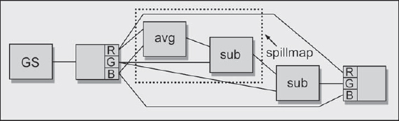
Figure 4-7: Despill Flowgraph: Green Limited by the Average of Red and Blue
There are several ways to perform the averaging operation indicated in the flow-graph. A brightness node can be used to scale the red and blue channels by 50 percent, and then they can be added together to make the average. A color curve node could be used to scale the red and blue channels by 50 percent, then add them together. The coolest way is to use a cross-dissolve node, which virtually any software will have. It takes two inputs (the red and blue channels in this case), and then allows you to set the degree of mix between them. If you set the mix percentage to 50 percent you will get the same average that the previous methods achieved. However, now you can easily try different mix percentages to see how they affect the despill results. Perhaps a 20/80 mix is better, or maybe a 60/40 mix will eliminate those pesky artifacts. Set to one extreme you have the green by red despill, and the other extreme will give you the green by blue. You now have an adjustable despill procedure.
4.3.4 Green Limited by Other Formulations
Because the despill operation is in fact logically invalid, perfect results are guaranteed never to happen. Fortunately, the residual discolorations are usually below the threshold of the client's powers of observation (the hero's shirt is a bit more yellow than on the set, for example). When the discolorations are objectionable, we are free to explore utterly new despill formulations since we know that they are all wrong. It is just a matter of finding a formulation that is not noticeably wrong in the critical areas on the particular shot you are working on at the moment. Here are a couple of arbitrary examples that illustrate some different alternatives.
- Limit green to 90 percent of the red channel.
This is a simple variation of the green limited by red despill flowgraph in Figure 4-4 and illustrates how easy it is to create infinitely varied despill operations. Again, the name of the game is to create a spillmap that, when subtracted from the green channel, will produce the results we want. If we want to limit the green to 90 percent of the red channel instead of the full red channel, then the red channel needs to take a bigger “bite” out of the green channel. We can do this simply by scaling the red channel by 0.9 before subtracting it from the green record to make the spillmap. This will make a 10 percent “thicker” spillmap, which will in turn take a 10 percent bigger bite out of the green record when it is subtracted, which limits the green channel to 90 percent of the red channel.
Figure 4-8 shows the complete flowgraph for the new and improved despill. One node has been added within the spillmap area (scale 0.9) that scales the red channel down to 90 percent of its original value. This lower red value is subtracted from the green channel in the next sub node, resulting in the “thicker” spillmap. In the following sub node this thicker spillmap is subtracted from the original green channel, lowering it 10 percent more than it would by simply limiting it to the red record.
- Limit green to exceeding the average of the red and blue by 10 percent.
This is a minor variation of the green limited by the average of red and blue de-spill shown in Figure 4-7. Keep in mind that even minor variations in the despill operation can produce large changes in the appearance of the despilled image. In this case, we want a spillmap that will let the green channel rise 10 percent above the average of the red and blue channels. This means that the spillmap needs to be 10 percent “thinner” than the simple red and blue average. If we scale the red and blue average up by 10 percent before subtracting it from the green channel, the results of the subtraction will be less, producing the thinner spillmap we want.
Figure 4-9 shows the complete flowgraph for the fancy new despill. One node has been added within the spillmap area (scale 1.1) that scales the red/blue average up by 10 percent. When this greater value is subtracted from the green channel in the next sub node, the result is the thinner spillmap we need. In the following sub node this thinner spillmap is subtracted from the original green channel, raising it 10 percent above the average of the red and blue channels.
The despill algorithms discussed so far are by no means the end of the list. Ultimatte doesn't say much about their green despill algorithm, but they do have an elaborate formulation for their blue despill. It is based on the observation that very saturated blues are rare in nature. Their blue despill rule goes like this: “If green is equal to or less than red, hold blue to the level of green. If green is greater than red, let blue exceed green only by the amount green exceeds red.”
Having done it myself, I can assure you that even this convoluted despill algorithm can be implemented in a channel math node or by discrete nodes in a flowgraph. The point of this arcane example is to point out that there are actually an unlimited number of possible despill algorithms, and to encourage you to explore and experiment. The spillmap is the key. Come up with a novel way of creating your own spillmap, then subtract it from the green channel to create your own custom despill algorithm.
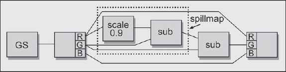
Figure 4-8: Despill Flowgraph: Green Limited to 90% of Red
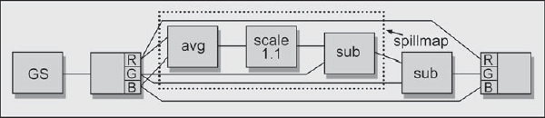
Figure 4-9: Despill Flowgraph: Green Limited to 10% above the Average of Red and Blue
4.4 Refining the Despill
Once you have discovered the despill algorithm that gives the best results for a given picture content, there is another layer of operations that can be performed to refine and improve the results even further. Here is a collection of refinement procedures you can try when the need arises. Keep in mind that they can all be used in combination with each other.
4.4.1 Channel Shifting
Shift the limiting channel (red or blue) up or down by adding or subtracting small values such as 0.05. This has the effect of not only increasing and decreasing the brightness of the spillmap, which increases and decreases how much spill is pulled out, but it also expands and contracts it in and out of the edges.
4.4.2 Spillmap Scaling
Using a scale RGB node or a color curve, scale the spillmap up or down to increase or decrease its spill removal. This will have a similar but somewhat different effect than channel shifting.
4.4.3 Mixing Despills
Set up two completely different despill operations—maybe one limited by red and the other limited by blue—and then use a cross-dissolve node to mix their outputs together. Try juggling the percentage mix back and forth to find the minimum offensive artifact point.
4.4.4 Matting Despills Together
You cannot find one despill operation that works for the whole picture. One despill operation works great for the hair, but a different one works for the skin. Create a traveling matte to split the two regions and composite the usable part of one and the usable part of the other. Divide and conquer.
4.4.5 Blue Degraining
It was mentioned that any green limiting that uses the blue record will emboss the blue channel's oversized grain into the green channel. This seems to happen most often on the smooth skin of beautiful women, for some reason. Simply degrain the blue channel to use in the spillmap calculations. Don't use the degrained blue channel in the final composite, of course. If you don't have a real degrain operation available, a small radius gaussian blur might help.
4.5 Unspill Operations
In all of the examples so far the strategy has been to create a green spillmap, and then subtract it from the green channel to pull the excess green out of the green-screen plate. This approach obviously removes some green from the image, which we want, but removing green also darkens, which we don't want. It also causes hue shifts, which we really don't want. Subtracting the excess green certainly gets the green out, but there is another way—we could just as well add red and blue. Either approach gets the green out. Since subtracting green is called despill, I call adding red and blue unspill in order to distinguish the two. This technique can solve some otherwise insoluble despill problems.
4.5.1 How to Set It Up
The basic idea is to create your best green spillmap, scale it down somewhat, subtract it from the green channel as usual, but also add the scaled spillmap to the red and blue channels. In fact, the spillmap is scaled appropriately for each channel. Since we are adding some red and blue, we do not want to pull as much green out as before, so we can't use the original spillmap at full strength on the green channel. For example, it might be scaled to 70 percent of its original brightness. For adding to the red channel, we might use 30 percent of it, and for the blue channel maybe 20 percent. The exact proportions totally depend on the picture content and the method used to create the spillmap.
Figure 4-10 shows a flowgraph for the unspill operation. Starting at the left, the greenscreen plate goes into a channel splitter node. The separated channels are used to create the spillmap, using your method of choice, which is represented by the “spillmap” node. The resulting one-channel spillmap is then fed into all three inputs of a channel-combining node to create a three-channel version of the spillmap. We now have a three-channel image with the same spillmap replicated in all three channels. This is just a convenience to feed the three-channel spillmap into a single “scale map” node where each channel can be scaled individually. The scaling can be done with a scale RGB node or a color curve. The “unspillmap” is then split into three separate channels again with the next channel splitter node so that each channel of the original greenscreen can get its own separate add or subtract operation with its own scaled version of the unspillmap. The unspilled channels are then recombined in the last node to make the final three-channel unspilled version of the greenscreen plate.
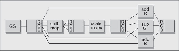
Figure 4-10: Flowgraph of Unspill Operation
This may look like a lot of nodes for a despill operation (excuse me, unspill operation), but you will think it well worth the trouble when you cannot get rid of those pink edges on the blonde hair. You might be able to use the unspill method for the entire plate, or you may find it more effective to mask off just the troublesome region of the picture for this special treatment.
4.5.2 Grading the Backing Color
How many times have you composited a picture only to find an ugly colored “fringe” around the foreground object? Perhaps you had a light gray fringe that glowed when you composited the foreground over a dark background, or a dark fringe when you composited it over a light background. You probably started eroding the matte to trim away the colored fringe only to find important edge detail disappearing along with the fringe. There is another approach that may help. It may be possible to change the color of the fringe to something that blends better with the background—perhaps a lighter or darker gray, or maybe some particular color, for example.
Remember Color Plate 47 discussed in Section 4.3.2, “Green Limited by Blue,” in which the three colored strips were placed over three slightly different green backing colors? When the despill operation was performed the three slightly different green backing colors suddenly became three very different colors, and the colors were different again depending on the despill method used (Color Plate 48 and Color Plate 49). Those “residual” backing colors blend with the edges of the foreground objects and contaminate them with their hue. If the greenscreen is brightly lit the edges will be light, and if it is dark the edges will be dark. This is the fringe that you see after your composite. If we could change the residual color of the backing, we would change the color of the fringe.
You can change the residual backing colors to whatever you want with the un-spill method. This is because the unspill method both lowers the green and raises the red and blue channels in the backing region. By scaling the spillmap appropriately for each channel, the red, green, and blue channels in the backing region can be set to virtually any color (or neutral gray) that you want. Another arrow for your quiver.