CHAPTER 10

Video

Film is a wonderfully simple medium in concept. A shutter flicks open for a fraction of a second, and a frame of film is exposed, capturing a moment of time in full color. If something happens to be moving, it naturally leaves an agreeable streak on the film to signal its motion. Video is not nearly so simple. Video suffers from a desperate need to pack the maximum picture into the minimum signal so it can be broadcast over the airwaves. All of the moving pictures must be squeezed into a single rapidly gyrating radio wave. This one fantastically high-pitched wave must carry a black and white picture, an overlay of all of its color, plus a little sound track tucked in on the side.

Even though one frame of video is packed into a tiny fraction of the space of a frame of film, it still looks surprisingly good. This is because the scientists and engineers who designed our modern video system very carefully placed the maximum picture information into the same parts of the visual spectrum as the most sensitive parts of human vision. There is a flurry of picture information wherever the eye can see fine detail. Where the eye is nearly blind, there is almost no picture information. Although they are brilliant in concept and execution, all of these compression techniques come at a price. They introduce artifacts.

Compared to an equivalent frame of film, each frame of video is degraded in a variety of subtle ways, both spatially and temporally, as carefully calculated sacrifices to data compression. These artifacts and defects are all neatly tucked away into the visual “corners” of the human perception system, but emerge to haunt you when the video is digitized and you try to manipulate it. Understanding the cause of each of these artifacts and how to compensate for them is the subject of this chapter.

10.1 Getting Video to and from a Workstation

The videotape that the client gives you could be analog or digital. Either way, it must become a digital image file on your workstation before you can do anything with it. There are two general approaches to getting the frames from tape to workstations. The first method is to use a digital disk recorder (DDR). The DDR is little more than a high-speed disk drive with some video circuitry. The video route using a DDR is shown in Figure 10-1. A videotape recorder (VTR) is connected to the DDR to play the videotape. The tape is played at normal speed and the video images are laid down on the DDR's disk drive in real time. A 10-second shot takes 10 seconds to lay down. The DDR will have two inputs, one for digital VTRs such as D1, and the other for analog VTRs such as BetaSP. The analog input will digitize the incoming video, whereas at the digital input it is already digital and just needs to be routed to the disk.

Figure 10-1: Video Route with DDR Setup

Once the video frames are on the DDR's disk, they can be transferred to the workstation as ordinary files over a network, such as Ethernet. When the shot is completed, the frames are transferred back to the DDR over the network, like any file. The transfer command includes information as to where on the DDR you would like the frames to be located. After the finished frames have all collected themselves on the DDR, the shot can be played back and viewed on a monitor in real time for review, then simply dubbed off to videotape on the same VTR that was used to load them.

The video capture card video route is illustrated in Figure 10-2, which is a lower-cost setup than the DDR. A special video card that is capable of digitizing incoming analog video in real time is installed in the workstation. If the input is digital video it is simply routed to the workstation disk drive. Once the video frames are on the disk drive they are available for compositing. When the finished shot is ready to go back to videotape, the video capture card can send the frames back to the tape recorder. Again, if it is an analog recorder, it will convert the digital files to analog for the VTR.

Figure 10-2: Video Route with Video Capture Card

10.2 How Video Works

Video is such a hideously complex medium to work with that simply memorizing a few rules or guidelines will not work. To be truly competent, you must actually understand it. This section describes how the video frame is put together in space and time and the artifacts this introduces to working with video. This background information is essential for understanding the rest of the chapter, which addresses the practical issues of how to deal with or work around those artifacts. After the operational principles of video are laid out, the difference between NTSC, the American television standard, and PAL, the European television standard, is described; they both use the same principles with just minor variations in frame size and frame rate.

The effort here is to avoid the usual video techno-babble and just describe the aspects of its operation that actually affect the digital manipulation of video images. It is video as seen from the digital compositor's point of view. As a result, it is mercifully incomplete. Knowing that it was invented by Philo T. Farnsworth and is encoded on a 3.58 megahertz subcarrier will not help you to pull a matte or resize a frame. Knowing how field interlacing works or how to compensate for the non-square pixels will. It contains everything you need to know, and nothing you don't. Let us begin.

10.2.1 Frame Construction

This section describes how a frame of video is constructed from interlaced fields and the troublesome effect this has on the motion blur of moving objects. This is essential information for understanding why and how to deal with interlaced images. Pixel data formation is also described because it is not a simple red, green, and blue data value for each pixel, even though a frame of video on your monitor appears to have typical RGB data. This has important implications for the amount of detail when pulling a matte.

10.2.1.1 The Scanning Raster

In this first approximation of the video frame, we introduce the concept of an idealized scanning raster. While film opens a single shutter to expose the entire frame at once, video is forced to peel the picture out serially one pixel at a time because it is being broadcast over a single carrier wave to the home TV receiver. It's like building up the scene a pixel at a time by viewing it through a tiny moving peephole, as shown in Figure 10-3. Real TV cameras, of course, do not physically scan scenes with raster beams. The image is focused on the back of the video capture tube, and there it is digitally scanned with a moving “raster.” The following description, then, is a helpful metaphor that will illuminate the problems and anomalies with interlacing and motion blur that follow.

The raster starts at the upper left-hand corner of the screen and scans to the right. When it gets to the right edge of the screen it turns off and snaps back to the left edge, drops down to the next scan line, and starts again. When it gets to the bottom of the frame the raster shuts off and snaps back to the upper left-hand corner to start all over again.

Figure 10-3: Digitizing a Scene to Video with a Scanning Raster Beam

This simple first approximation is not practical in the real world because it generates too much data to be transmitted over the limited bandwidth of the video carrier wave. A way had to be found to reduce the amount of transmitted data in a way that would not degrade the picture too much. Simply cutting the frame rate in half from 30 fps to 15 fps would not work because the frame rate would be too slow for the eye to integrate the frames into smooth continuous motion. To solve this little problem, the clever video engineers at NTSC introduced the concept of interlaced video, in which only half the picture is scanned each frame, reducing the demands on the electronics and the signal bandwidth for broadcast. But this half of the picture is not half as in the top or bottom half, but half as in every other scan line.

10.2.1.2 Interlaced Fields

Interlacing means that it takes two separate scans of the scene, called fields, which are merged together to make one frame of video. Field 1 scans the entire scene from top to bottom, but only the odd scan lines. Starting with the first scan line of active video (ignoring vertical blanking and other scan line activities that have nothing whatsoever to do with the picture you see on your monitor), it then scans lines 3, 5, 7, 9, and so on to the bottom of the frame. The raster snaps back to the top and field 2 rescans the entire scene from top to bottom again, but this time scans only the even scan lines, starting with line 2, then 4, 6, 8, and so on. These two fields are then merged, or interlaced, together on the TV screen to form a complete video frame.

Figure 10-4 illustrates how field 1 and field 2 are interlaced to make a full video frame. (The number of scan lines has been reduced to just 28 for clarity.) If the field 1 and field 2 pictures in Figure 10-4 were slid together they would fill in each other's blank lines to make a full picture. The reason this does not (usually) flicker is due to a combination of the persistence of vision and the “persistence” of the TV monitor. Each field stays glowing on the screen for a few milliseconds after it has been drawn by the raster, fading slowly (electronically speaking). So while field 1 is still up, field 2 is being drawn between its scan lines. While field 2 is slowly decaying, the next field 1 writes between its scan lines, and so on. These interlaced fields rapidly replace each other and blend together to form continuous motion to the eye.

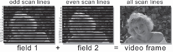
Figure 10-4: Even and Odd Scan Lines of Field 1 and Field 2 Combine to Make One Video Frame

10.2.1.3 Effects on Motion Blur

Interlacing even and odd fields was a wonderful ploy to cut down on the required bandwidth to broadcast the TV picture, but it brought with it some hideous artifacts. One example is the motion blur on moving objects. Think about it. With film, the shutter opens, the object moves, and it “smears” across the film frame for the duration of the shutter time—simple, easy to understand, and looks nice. With video, there is a continuously scanning raster spot that crosses the moving object many times per field, and with each crossing the object has moved to a slightly different location. Then it starts over again to scan the same frame for the next field but the object is in yet another whole place and time. Suffice it to say, this results in some rather bizarre motion blur effects on the picture. This all works fine when displayed on an interlaced video system, but creates havoc when trying to digitally manipulate the fields while they are integrated as static frames.

Let's take a look at how horizontal motion blur works with interlaced video fields. Figure 10-5 illustrates a simple ball moving horizontally which we will “photograph” in motion with both film and video. With film, the ball's motion with the shutter open smears its image horizontally, as shown in Figure 10-6. A simple and intuitive result. With interlaced video, the ball is captured at two moments during the video frame, appearing in two places. Worse, the two images are split between the odd and even lines, so the odd set of lines (field 1) shows the ball at an earlier moment, and the even lines (field 2) show the ball at a later moment (as in Figure 10-7). It's like looking at the scene twice through a Venetian blind that somebody is shuttering open and closed.

In the next case let's look at vertical motion blur as seen by film and video. The original ball moving vertically is depicted in Figure 10-8. Its film version can be seen in Figure 10-9 with a nice vertical motion blur, similar to the film motion blur of the horizontal ball. But once again, the interlaced video fields present some bizarre anomalies in Figure 10-10, and for the same reason as in the horizontal example. The ball was photographed twice in each frame in a slightly different position, and the two snapshots were interlaced by even and odd lines. When it comes time to operate on these images, these interlace artifacts must be properly addressed or the results will be truly awful.

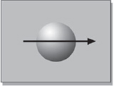
Figure 10-5: Object Moving Horizontally

Figure 10-6: Film Motion Blur

Figure 10-7: Interlaced Video Fields Motion Blur

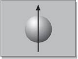
Figure 10-8: Object Moving Vertically

Figure 10-9: Film Motion Blur

Figure 10-10: Interlaced Video Fields Motion Blur

10.2.1.4 Field Dominance

This may sound like an unnecessary techno-video detail, but believe me, if you ever get it wrong on a project you will be extremely glad that you know about it. You will be able to turn calamity into heroism with practically a flick of a switch. We saw in the previous section how field 1 is interlaced with field 2 to make a full frame of video. But a video camera is a continuously running device. In point of fact, it is not putting out full “frames,” but continuous alternating fields. The only thing that distinguishes field 1 from field 2 is whether it starts on even or odd scan lines. To the eye, it is a continuous series of fields. This means that you could just as easily make a video frame from a field 2 followed by the next field 1. Nothing in the normal video pipeline would be harmed by this. Until you digitized the video to a workstation, that is.

When the video is digitized to a workstation it is no longer a continuous stream of fields. The video fields are now “frozen” and paired together to make video frames. Normally, each video frame would consist of a field 1 followed by the next field 2, as shown in Figure 10-11. This is called field 1 dominance. If, however, you delayed the digitizing until the start of field 2, each video frame would now consist of a field 2 followed by the next field 1. This would be field 2 dominance. These field 2 dominant frames would look fine on your workstation because you are not viewing them with an interlaced video monitor. Your workstation monitor is a progressive scan, meaning that it scans every scan line from top to bottom once. Even a local “movie” played on your workstation will look fine—until you send it back to the video monitor anyway.

Figure 10-11: Field Dominance

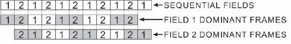
When images are sent to a DDR the scan lines are laid down just like they are on your system. The top scan line, being odd, goes to field 1, and the second scan line, being even, goes to field 2, and so on. The problem here is that the system assumes that the field 1 of each frame is the field 1 that comes before the field 2 of that frame, not after. If your digitized video was field 2 dominant, each field 1 actually belongs to the following frame of video, which is a moment later in time, rather than a moment earlier. The transfer utility that sends the frames from your workstation to the DDR knows nothing of this and assumes the field 1 comes before the field 2, not after. As a result, the two fields get swapped in time on the DDR. When you play the video, any motion in the picture has a wildly jerky appearance because the action is literally taking two steps forward followed by one step backward—a calamity of the first order.

To confirm that you have a field dominance problem, put the DDR in single field mode and single step through the video to follow the action. The motion will literally take one step forward, then one step backwards. This is your conclusive test. Now you get to be the hero. Announce to your stunned clients and colleagues that there is simply a field dominance problem and you will have it fixed shortly. The fastest and simplest fix is to switch the field dominance in the utility that transfers the frames from your workstation to the DDR. If that is technically or politically impossible, then the original video will have to be transferred to your workstation again with the dominance switched.

10.2.1.5 Color Resolution

You might reasonably assume that when you are looking at a 720 × 486 frame of NTSC video in RGB mode on your workstation you have 720 × 486 pixels of red, green, and blue. Of course, that would be wrong. Again, the contortions here are another data compression scheme to again reduce the bandwidth required to broadcast the picture. It is based on the observation that the eye is much more sensitive to detail in luminance (brightness) than it is to color. Why pack more color information into the image than the eye can see?

To take advantage of the eye's reduced sensitivity to color, the RGB image in the video camera is converted into another form upon output called YUV. It is still a three-channel image, but instead of one channel for each color, the YUV channels are mathematical mixes of the RGB channels. The “Y” channel is luminance only— what you would get if you took an RGB image and completely desaturated it to a grayscale image. All of the color information is mixed together in a complex way and placed in the “U” and “V” channels, which are referred to as “chrominance.” The hue is not stored in one channel and the saturation in the other. One channel carries the hue and saturation for orange-cyan colors, while the hue and saturation for yellow-green-purple are in the other.

Now that the video signal is converted to one channel of luminance and two channels of chrominance the data compression can begin. Since the eye is most sensitive to luminance, it is digitized at full resolution. Since the eye is less sensitive to the chrominance part of the picture, the two chrominance channels are digitized at half resolution. The digitizing of these three channels is referred to as 4:2:2, which is four samples of luminance for every two samples of one chrominance channel and two samples of the other chrominance channel. This means that a YUV frame consists of a luminance channel that is full resolution, plus two chrominance channels at half resolution. This results in a full frame of picture with the equivalent of just two channels of data, instead of three channels, like true RGB image formats. This lightens the data load by one third, resulting in a compression of 1.5 to 1.

Figure 10-12 illustrates the difference between a true RGB image and a YUV image. A short “scan line” of four pixels is illustrated for each. For the RGB image, all four pixels have unique data values in each channel. The YUV image does not. The Y (luminance) channel has four unique pixel values, but the U and V channels have only two chrominance data values each to span the four Y pixels.

This is obviously a bad omen for any chrominance (color)-based operation, such as pulling a bluescreen matte. The matte will have a serious case of the jaggies. The situation is not quit as bad as it seems from Figure 10-12, however. Since the Y channel is full res, when a YUV image is converted to RGB for the workstation each pixel does inherit some detail from it across all three channels. But this detail is a mathematical interpolation rather than the result of a direct digitizing of the original scene, so there is some loss of information, and therefore detail. A picture photographed with a film camera, then digitized to 24 bits RGB and resized to video resolution, will contain more fine detail than a 4:2:2 YUV version converted to RGB, even though they are both the same resolution and file size. You can't fool Mother Nature.

If you can have the film re-digitized with a 4:4:4 sampling, you will see a very big improvement in the matte's blocky pixels compared to what you got with the 4:2:2 digitizing. With 4:4:4 digitizing the U and V channels, like the Y channel, are scanned at full resolution.

Figure 10-12: Color Resolution of RGB versus YUV

10.2.2 NTSC and PAL Differences

NTSC (National Television Systems Committee) is American and PAL (Phase-Alternating Line) is European. They both operate under the principles described in the previous section, but there are important differences in the number of scan lines in a frame, frame rate, and pixel aspect ratios. Yes, video pixels are not square, so video frames become distorted when displayed on the square pixel monitor of your workstation.

10.2.2.1 Frame Rate

10.2.2.1.1 NTSC

NTSC video runs at 30 frames per second (fps), consisting of 60 interlaced fields per second. Well, sort of. Like all things video, there is more to it than that. It really runs at 29.97 frames per second. The reason for the slight discrepancy is that when TV went color in 1953, signal timings had to be juggled a bit to make things come out even, and 29.97 frames per second is the result. What effect does this have on you? Usually, none. However, you might want to know about drop frame time code, just in case you trip over it one day.

10.2.2.1.2 Drop Frame Time Code

Professional video standards have a continuously running time code embedded with the video images on a separate track in the format hours:minutes:seconds:frames. The problem is that if you run your time code clock on the assumption that there are exactly 30 frames per second when there are really 29.97, after half a minute your time code will be over-long by one frame. In one minute it will be over-long by two frames, and so on. The fix for this continuously drifting clock time problem is to drop a couple of frames out of the time code every minute—hence the term drop frame time code. Because commercials are so short, they normally use non-drop frame time code.

So how does this affect you? Two ways. First, when the client delivers a videotape you must ask if it is drop frame or non-drop frame, because it slightly changes the total number of frames you have to work with. Two tapes of the same run time, one drop frame and the other non-drop frame, will be off by two frames after one minute. This variable timing issue will also wreak havoc if you mix drop and non-drop video elements, then try to line them up based on their time codes. The second issue is that whenever you have to deliver a videotape to the client you should always ask if the tape should be drop or non-drop frame time code.

10.2.2.1.3 PAL

PAL video runs at exactly 25 frames per second (fps), consisting of 50 interlaced fields per second. There is no drop/non-drop frame time code issue with PAL because it runs at exactly the advertised frame rate.

10.2.2.2 Image Size

10.2.2.2.1 NTSC

A digitized NTSC frame is 720 × 486. That is to say, each scan line is digitized to 720 pixels, and there are 486 active scan lines of video. In truth, of the 720 pixels only 711 are picture and the remaining nine are black. For the sake of simplifying all calculations, we will assume that all 720 pixels are picture. This introduces an error of only around 1 percent, which is far below the threshold of visibility in video. The aspect ratio of the NTSC image as displayed on a TV screen is 4:3 (1.33).

10.2.2.2.2 PAL

A digitized PAL frame is 720 × 576. That is to say, each scan line is digitized to 720 pixels, and there are 576 active scan lines of video. In truth, of the 720 pixels only 702 are picture and the remaining 18 are black. For the sake of simplifying all calculations, we will assume all 720 pixels are picture. Again, this introduces an error of only around 1 percent, which is far below the threshold of visibility in video. The aspect ratio of the PAL image as displayed on a TV screen is 4:3 (1.33).

10.2.2.3 Pixel Aspect Ratio

If you calculate the image aspect ratio based on the image size data given in the previous section for video frames, you will get a rude surprise. While both the PAL and NTSC video images are supposed to have an aspect ratio of 1.33, when you do the math for NTSC you get an aspect ratio of (720 ÷ 486) = 1.48, and for PAL you get an aspect ratio of (720 ÷ 576 = ) 1.25. This is because neither PAL nor NTSC has square pixels! However, your workstation does have square pixels, and this introduces a number of messy problems. This section describes how the non-square pixels work, and how to compensate for them will be covered in Section 10.4.3, “Non-Square Pixels.”

10.2.2.3.1 NTSC

The aspect ratio of a pixel in NTSC is 0.9. That is to say, the pixels are 10 percent narrower than they are tall. Here's the story. The video frame has a very specific number of scan lines—exactly 525, of which exactly 486 contain picture, which is what we work with and therefore all we care about. One cannot arbitrarily increase or decrease the digitizing resolution vertically—there must be exactly one scan line of data to one scan line of video. There are no such hard barriers horizontally, however. The original analog video signal could be digitized horizontally at any desired resolution, limited only by the speed of the hardware. It was decided to digitize each scan line to 720 pixels as the best compromise between limiting data bandwidth and visual sufficiency.

This means, however, that the video is digitized more finely horizontally than vertically. If the horizontal digitizing resolution matched the vertical resolution to make square pixels, then each scan line would be digitized to about 648 pixels instead of 720. None of this causes a problem until you display a video image on your workstation monitor. When you do, the image suddenly stretches 10 percent horizontally.

Figure 10-13 illustrates what happens when a video image with non-square pixels is displayed on a workstation monitor that has square pixels (all effects have been exaggerated for the sake of clarity). Note that the circle on the video monitor on the left was perfectly round, but becomes stretched when displayed with the square pixels of the workstation. This stretching of the image has a couple of implications, which will also be addressed in Section 10.4.3, “Non-Square Pixels.”

10.2.2.3.2 PAL

The aspect ratio of a pixel in PAL is 1.1. That is to say, the pixels are 10 percent wider than they are tall. PAL is digitized to the same 720 pixels that NTSC is, but it has 576 scan lines of picture compared to NTSC's 486. When placed on a video monitor the PAL image is squeezed vertically, making its pixels wide. NTSC is squeezed horizontally, making its pixels tall. When a PAL image is displayed on the square pixel display of a workstation monitor it stretches vertically, which would make the circle in Figure 10-13 tall and skinny.

10.2.2.4 Country Standards

There are basically three world television standards distributed roughly by the political affiliations of the inventing countries. NTSC, invented in America, is prevalent in countries that are our neighbors and allies. PAL was invented in Europe, so is most prevalent there. The French, of course, had to develop their own television standard (SECAM) to preserve and protect their cultural uniqueness. The old USSR, unable to develop their own, opted to adopt the French SECAM format because of its singular virtue of being neither American nor European. You see, France is not really Europe. It's France.

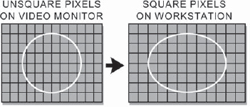
Figure 10-13: NTSC Image Stretches 10% Horizontally When Viewed on a Workstation Monitor

Following is a partial list for ready reference of the most prevalent countries that you might be doing business with. If you find yourself doing effects for Zimbabwe, you will have to look them up in a world television standards reference.

NTSC: America, Japan, Taiwan, Canada, Mexico, most of Central and South America

PAL: United Kingdom, Australia, China, Germany, Italy, and most of Europe

SECAM: France, Russia, and most of the old communist world

10.2.3 Types of Video

In addition to the exciting challenges offered by interlaced fields and non-square pixels, video also comes in a variety of types. Component video is better because it contains more information for digital manipulation. Composite video is necessary for broadcast. Some video formats are digital, others analog. Here we define each of these types with just enough depth to enable you to understand the various video formats, which is the topic of the following section. I told you video was hideously complex. Did I lie?

10.2.3.1 Component Video

A video camera shoots a scene as an RGB image internally but converts the video to YUV on output for videotaping as described in Section 10.2.1.5, “Color Resolution.” When the video is in this format it is referred to as component video because the video is separated into its luminance and chrominance components. In fact, this is the form of video we have been discussing all along. It is the highest resolution of video data and is the best for digital compositing.

10.2.3.2 Composite Video

Component video is unsuitable for broadcast because it is a three-channel format. It needs to be encoded into a single-channel format so it can be used to modulate a single carrier wave for broadcast purposes. When component video is encoded into a single channel like this it is referred to as composite video because it is a composite of the three components. This encoding process is yet another data compression scheme, and it both introduces artifacts and degrades the quality of the picture yet again compared to the original component version.

For composite video to be digitized for a workstation it must first be decoded through a transcoder to convert it back to component (YUV), then converted to RGB. The resulting RGB image does not have the sharpness and color detail of the original component version.

10.2.3.3 Digital and Analog

Not only does video come in component and composite formats, but there are analog and digital versions of each. The video signal in an analog format is laid down on tape as a continuously oscillating analog signal from the video camera, somewhat like an audio tape cassette. In order to become digitized to a workstation, the analog tape deck is connected to the analog inputs of a DDR, which digitizes the video to its disk as it is played. This digitized form can then be converted to RGB and sent to the workstation. Successive copies (dubs) of an analog tape degrade with each generation, and digitizing the tape several times will produce slightly differing results each time due to variations in reading the analog signal with each playing.

For a digital video format the video signal is laid down on tape as digital data, somewhat like a computer data tape. The tape's magnetic medium records only a series of 1’s and 0’s instead of the continuously oscillating signal of the analog formats. When a digital tape is laid off to a DDR it is connected to the digital inputs and the data is simply copied from the tape to the DDR. Successive copies (clones) of a digital tape do not degrade with each generation, and laying the video down to a DDR several times will produce identical results because it is simply copying the same digital data with each playing.

In reality, of course, digital tape formats are not totally flawless and unlimited clones cannot be made. The truth is that errors on the magnetic tape do occur, so digital formats include robust error detection and correction/concealment operations. When an error is detected, the error correction logic attempts to reconstruct the bad pixel from error correction data on the tape. If that fails, the error concealment logic takes over and creates a replacement by averaging adjacent pixels. This, of course, is not an exact replacement of the bad pixel, but is designed to go unnoticed.

10.2.3.4 Interlaced versus Progressive Scan

In Section 10.2.1.2, “Interlaced Fields,” we learned of the horrors of interlaced video. Since the video cameras scan the scene with an interlaced scanning raster, the tape recorders must lay the video down in the same interlaced format. As we saw, this interlaced scan technique introduces a number of problems from bizarre motion blur artifacts to field dominance hassles. The fact that the video world has gone digital and the growing interest in using high-resolution video cameras to shoot movies have combined to motivate the video industry to begin development of progressive scan video cameras.

Progressive scan video cameras simply scan the scene once from the top down, just as common sense would dictate, and rather like a movie camera. A video camera that records at 24 frames per second with a progressive scan is referred to as a “24P” camera. The use of these progressive scan video cameras for the video capture of elements that are to be digitally manipulated will eliminate the problems that interlaced scanning introduces.

10.2.4 Video Formats

Here is where we pull it all together to get specific about the most prominent video formats you are likely to encounter. They are described in terms of being component, composite, analog, or digital, plus a few words on their intended applications and how good the picture quality is for compositing.

10.2.4.1 The All-Digital Formats

This is a listing of the major all-digital professional videotape formats. There are several manufacturers that make various models of these videotape machines.

D1: A component digital format using a 19mm wide tape. This is the current standard for studio and postproduction work, where the extra data precision is needed to retain quality during digital manipulation.

D2: A composite digital format using a 19mm wide tape. This is the current standard for television production and broadcast. Accepts analog and digital inputs. The analog input is digitized internally. Output is both analog and digital.

D3: A composite digital format using 1/2-inch wide tape. Accepts analog and digital inputs. The analog input is digitized internally. Output is both analog and digital.

D4: No such format. Legend has it that Sony, being a Japanese company, decided to skip this model number because the number 4 is unlucky in Japanese culture, rather like the number 13 in Western cultures.

D5: A component digital format using 1/2-inch wide tape. Supports the NTSC and PAL standards. Also has an HDTV mode with about a 5:1 compression. In the HDTV mode the frame size is 1920 × 1080 with square pixels.

D6: An uncompressed HDTV interlaced and progressive scan format using a 19mm tape. Primary use is for electronic theater projection. Frame size is 1920 × 1080 with square pixels.

10.2.4.2 Sony

Sony struck off on its own and developed its own videotape standards, referred to as the beta format. They are all component formats for professional applications.

Beta: An analog component format using 1/2-inch wide tape. Fair quality, mostly used for ENG (Electronic News Gathering).

BetaSP: An analog component format using 1/2-inch wide tape. It is a higher-quality version of the Beta format. It is a very good-quality source of video for an analog format.

Digibeta: Digital Betacam. A digital component format using 1/2-inch wide tape. It is a high-quality source of video, even though it has about a 2.5:1 data compression, but D1 is better.

10.2.4.3 Consumer/Commercial

These formats are for the home consumer or the industrial commercial market. None of these formats is suitable for broadcast work. Nevertheless, a client may provide one because it is all they have.

VHS: The standard analog composite format for the consumer using a 1/2-inch wide tape. Low quality.

SHVS: An analog component format for the high-end consumer or commercial applications using 1/2-inch wide tape. As a component format it is higher quality than plain VHS.

U-Matic: An ancient analog composite format for commercial applications using a 3/4-inch wide tape. Low quality, but better than VHS.

DV: A digital component format for high-end consumer and low-end commercial applications using 8mm wide tape. Uses a very effective DCT (discrete cosine transform) compression scheme. Best quality of the nonprofessional standards.

10.2.4.4 HiDef

HiDef video is actually a collection of standards. Common to all of them is that they are digital, have square pixels, and have a 16:9 (1.78) aspect ratio picture. The variables are the image size, scan mode, and frame rate. While there are more variations than you would care to know about, Table 10-1 shows the ones you are most likely to encounter.

10.3 Telecine

Even if you work only in video, most of your video was probably shot on film and then transferred to video on a machine called a telecine (tell-a-sinny). These video frames are profoundly different from the video frames shot with a video camera. You need to understand how and why, so you can cope. Also, the client may turn to you for recommendations on the appropriate telecine setups for the best video transfer for your upcoming project together, so you need to be acquainted with a few telecine terms and procedures.

10.3.1 The 3:2 Pull-Down

There is no getting around the fact that film runs at 24 frames per second and video runs at 30 frames per second. One second of film must become one second of video, which means that somehow 24 frames of film have to be mapped into 30 frames of video. Some folks call it the “cine-expand.” The technique used to do this has historically been called the 3:2 pull-down, although some refer to it as the 2:3 pull-down. It is a clever pattern that distributes the film frames across a variable number of video fields until everything comes out even.

Seeking the lowest common denominator, we can divide both the 24 fps of film and 30 fps of video by 6, which simplifies the problem down to requiring that every 4 frames of film be mapped into 5 frames of video. This is done by taking advantage of the video fields. In the 5 frames of video there are actually 10 fields, so what we really need to think about is how to distribute the 4 frames of film across 10 fields of video.

Table 10-1: HiDef Video Standards
Image size	Scan mode	Frame rate
1920 × 1080	Progressive	24, 25, 30
1920 × 1080	Interlaced	25, 30
1280 × 720	Progressive	24, 30, 60
1280 × 720	Interlaced	30

The trick to putting 4 frames of film into 10 video fields is done with the film shutter pull-down. When the film is transferred to video, the film's electronic shutter is pulled down for each video field (there is no actual shutter—it is just a helpful metaphor for us non-telecine operators). To put one frame of film into one frame of video the shutter would be pulled down twice—once for field 1 and once for field 2. But what if we pulled the shutter down 3 times on the same frame of film, laying it down to 3 successive video fields? That frame of film would actually appear in 1½ frames of video. We could put one frame of film into 2 fields, the next frame of film into 3 fields, the third frame into 2 fields, and the fourth into 3 fields. Four frames of film are now laid into 10 fields, making 5 frames of video. For some odd reason, the eye does not notice the stutter step in the duplicate video fields, and the action blends smoothly.

Figure 10-14 illustrates the 3:2 pull-down pattern for one full cycle. The film frames are labeled A, B, C, and D, and each has a unique video field pattern. Frame A, for example, is the only one that exactly maps to one video frame by laying only on field 1 and field 2 of the same video frame. Note that the film frames have no compunction about starting or ending in the middle of a video frame. Film frame B, for example, ends in the middle of video frame 3, while film frame C is a two-field frame that starts in the middle of video frame 3.

Viewing the situation from the video side, if you single-step through these frames on your workstation you will see a repeating pattern of “clean” and “mixed” video frames. The mixed video frames have a different film frame in each field, so the action is “fragged” along scan lines, like the interlace motion blur shown in Figure 10-7. The clean frames have the same film frame in both fields. From the pattern of clean and mixed video frames in Figure 10-14 you can see that once you find the two adjacent mixed frames you know you are on video frames 3 and 4. From there you can back up 2 frames and know that you are on video frame 1, the A frame of film.

10.3.2 Pin Registration

Although all telecines move the film using the sprocket holes, at the gate where the film frame is digitized there may or may not be any registration pins to hold the film frame steady and register it accurately while it is being scanned. As a result, the video frames may wobble (gate weave) or chatter a bit, depending on how well adjusted the telecine's film transport mechanism is. In fact, if you watch the corners of your TV while a movie is playing you can sometimes actually see this gate weave. For normal TV viewing of the movie of the week, this is not a problem. For compositing, however, it is.

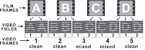
Figure 10-14: The 3:2 Pull-Down Pattern for Transferring Film to Video

You cannot composite a nice steady title or graphic over a wobbling background layer, or worse, two wobbling layers over each other. If you do not want to have to stabilize your elements before compositing (which takes time and softens the images), then you want video that was transferred on a pin-registered telecine.

10.3.3 Recommendations to the Client

Ideally, you will have a chance to talk to the client about the job before the film has been transferred to video. This way you can give the client some tips on how best to transfer the film to video for a happy compositing experience. The two big issues you want dealt with are a pin-registered telecine and no 3:2 pull-down.

A pin-registered transfer costs the client a bit more than a non-pin-registered transfer. Just point out that if you have to stabilize the video the filtering used to reposition the frame softens the image. If the client is unmoved by the reduced quality argument, then hit her with the big guns—you will charge her three times as much as a pin-registered telecine costs to stabilize the video. Voilà! A pin-registered transfer.

The other issue is the 3:2 pull-down—you don't want one because you will just have to spend time and trouble to remove it. If you are working on a Flame system it has such elegant tools for removing the 3:2 pull-down that this is not a real issue. If you are working with a generic compositing software package on a workstation, however, it is a big deal. The real problem here is actually communicating with the client. Although all digital compositors are highly qualified experts in their field, in film and video production there are, uhm, “variations” in skill levels. When talking to someone who does not even know what a 3:2 pull-down is, you may have to express the request a couple of different ways until the client gets it. Try each of the following phrases until the light bulb goes on.

1. A 30 frame per second transfer: This is the professionally correct form of the request to the telecine operator. It means that 30 frames of film are laid down to one second of video rather than the usual 24 frames per second; hence no 3:2 pull-down is needed. This is not as bizarre a request as it might seem, since many TV commercials are actually filmed at 30 fps, then transferred to video at 30 fps.
2. A one-to-one transfer: This would be one frame of film to one frame of video, hence no 3:2 pull-down.
3. No cine-expand: Do not expand (stretch) the cine (film) to make the 24 film frames cover 30 video frames.
4. No 3:2 pull-down: Could it be clearer than this?

One other telecine issue to be mindful of is over-exuberant image sharpening. When a telecine gets old, the operators might crank up the image sharpening to compensate. This can introduce ringing edge artifacts and also punch up the grain, which will be much more noticeable on a still frame on your workstation than on the moving footage on a video monitor. Advise the client to make sure this is not overdone because there is no image processing algorithm that can back out this edge artifact.

There is also noise reduction. This is another adjustable setting on the telecine process. While it is reducing noise (grain) in the transferred video, it also softens the image, so it must not be overdone, either. If the video needs softening, it is better to do it on the workstation where it can be tweaked as necessary. If it is laid into the video at telecine, you are stuck with it. Another artifact that excessive noise reduction can introduce is a “ghost” printing of one frame over the next.

Advise the client to make sure that the telecine transfer is as optimized as it can be for the following digital compositing operations. This way you won't inherit a set of utterly avoidable problems at the workstation that increases your production time (increasing costs) and lowers overall quality.

10.4 Working with Video

Now we will take all of the fascinating things we have learned about how video works and see how to work around all of the problems that video introduces to compositing and digital manipulation. Now that you know all about interlacing, we will see how to get rid of it. Now that you understand the 3:2 pull-down, we will see how to pull it up. And now that you are comfortable with non-square pixels, we will develop ways to work around them.

All of the following procedures and techniques are intended for compositors working with video frames on a conventional workstation with some brand of compositing software. If you are using Flame or an online video effects system such as a Harry you could actually skip this section, because they have internal automatic processes to hide the complexity of video from the operators.

10.4.1 De-Interlacing

If the video was mastered (shot) on video, the video frames are all interlaced and will probably need to be de-interlaced before you can proceed. If you are simply going to pull mattes, color correct, and composite, then de-interlacing won't be necessary. De-interlacing is necessary if there is any filtering of the pixels. Filtering (re-sampling) operations are used in translations, scales, rotations, blurs, and sharpening. Integer pixel shift operations such as moving the image up one scan line or over two pixels do not require filtering. To convince yourself of the need for de-interlacing, just take an action frame of interlaced video with visible motion blur and rotate it 5 degrees and observe the carnage.

There are three de-interlacing strategies. They vary in complexity and quality and, of course, the most complex gives the best quality. The nature of the source frames, the requirements of the job, and the capabilities of your software will determine the best approach. The reason for having all of these different approaches is in order to have as many “arrows in your quiver” as possible. There are many ways to skin a cat, and the more methods you have at your disposal the better you can skin different kinds of cats, or something like that. Gosh, I hope you are not a cat lover.

10.4.1.1 Scan Line Interpolation

This is the simplest and, not surprisingly, the lowest-quality method. The idea is to discard one field from each frame of video (field 2, for example), then interpolate the scan lines of the remaining field to fill in the missing scan lines.

Figure 10-15 illustrates the sequence of operations for scan line interpolation. A single field is selected from each video frame, then the missing scan lines are interpolated. The example in Figure 10-15 looks particularly awful because simple scan line duplication was used instead of a nice interpolation algorithm to illustrate the degraded image that results. Good compositing software offers a choice of scan line interpolation algorithms, so a few tests are in order to determine which looks best with the actual footage. This approach suffers from the simple fact that half of the picture information is thrown away and no amount of clever interpolation can put it back. The interpolation can look pretty good, even satisfactory, but it is certainly a quality level down from the original video frame.

10.4.1.2 Field Averaging

This next method retains more of the original picture quality, but is a bit more complex.

Figure 10-16 illustrates the sequence of operations for field averaging. Starting at the left, the frame is separated into its two fields. Each field gets the scan line interpolation treatment, making two full interpolated frames of video. These two frames are then averaged together to make the final frame.

Although this looks better than the simple scan line interpolation method does, it is still not as good as the original frame. Technically, all of the original picture information has been retained, but it has been interpolated and then averaged back together, slightly muddling the original image. Details will look sharper with this technique, but fast action can have a “double printed” look which might be objectionable. A test should be done and sent to the DDR for real-time playback on an interlaced video monitor to determine the best results for the actual picture content of the shot.

Figure 10-15: (a) Original Frame; (b) Single Field; (c) Interpolated Scan Lines

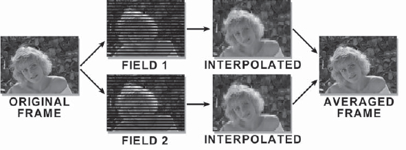
Figure 10-16: De-Interlacing with Field Averaging

10.4.1.3 Field Separation

The previous methods degrade the quality of the video image somewhat because the video fields are interpolated in various ways, losing picture information. This method retains all of the picture information and thus offers the best quality. It is also much more complicated. Illustrated in Figure 10-17, the idea is to separate the fields of each frame, performing no interpolations, then to use the separated fields as new frames. In essence, the video has been converted into a 60 “frame” per second movie. Although there is no degradation from frame interpolation, a number of messy complications have been introduced.

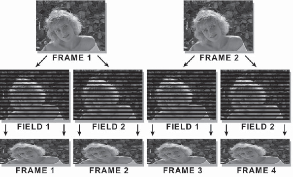
Figure 10-17: De-Interlacing with Field Separation

Each new “frame” is one-half of its original height due to half of its scan lines being missing, and the number of frames has been doubled. Both of these issues add complications to the job, but again, all of the picture data is retained. After the compositing is done with the “short frames,” they are re-interlaced before being sent to the DDR in exactly the same field order as they were de-interlaced. Watch your field dominance. Review Section 10.2.1.4, “Field Dominance,” for a refresher, if necessary.

Okay, now for the bad news. Since the short frames are half-height, all geometric operations must be done half as much in Y as in X. For example, to scale the image by 20 percent overall, you have to scale by 20 percent in X but only 10 percent in Y. The reason is that these short frames will become stretched in Y by a factor of two when re-interlaced, so all operations in Y will become doubled. The same holds for blurs and translations—half as much in Y as in X. Rotations are a special case. If you must rotate, the frame must first be scaled by two in Y to “square up” the image, rotated, then scaled back to half-height. A bit of a hassle, to be sure, but if maximum detail retention is the major concern, this is the way to go. Again, dedicated video systems like Flame and digital video effects switchers have built-in features that take care of these issues automatically.

10.4.2 The 3:2 Pull-Up

If the video was mastered on film and then transferred to video at 24 fps, the only interlaced frames will be the pull-down frames. The 3:2 pull-down frames will probably have to be removed with a 3:2 pull-up before proceeding. If you are simply going to pull mattes, color correct, and composite, then the 3:2 pull-up won't be necessary. The pull-up is necessary if there is any filtering of the pixels. Filtering (re-sampling) operations are used in translations, scales, rotations, blurs, and sharpening. The following procedures will make no sense whatsoever unless you are familiar with the information in Section 10.3.1, “The 3:2 Pull-Down.”

The 3:2 pull-up introduces the problem that the number of frames in the shot are reduced by 20 percent, which throws off any video time code information you may have been given. A little arithmetic can correct the timing information, however, by multiplying all times by 0.8 for the pull-up version of the shot. A further timing issue is that time code for video is based on 30 frames per second, and when the shot is pulled up it once again becomes 24 frames per second. As a result, some video time codes will land in the cracks between the film frames, making the exact timing ambiguous.

Ideally, your software will have a 3:2 pull-up feature and your troubles will be limited to discovering which of the five possible pull-up patterns you are working with and the timing information now requiring a correction factor. Watch out for changes in the pull-up pattern when the video cuts to another scene. If the film was edited together first, then transferred to video continuously (like a movie), then the pull-up pattern will be constant. If the film was transferred to video and then the video was edited (like a commercial), each scene will have its own pull-up pattern.

If your software does not have a 3:2 pull-up feature, you will have to “roll your own.” By studying Figure 10-14 in Section 10.3.1, “The 3:2 Pull-Down,” a painful but suitable procedure can be worked out. The hard part will be to determine the “phasing” of your shot—where the pattern starts, the “A” frame. Looking closely at the video fields in Figure 10-14, you will see a pattern of “clean” frames with no interlacing and “mixed” frames with interlacing. Reading video frames 1 through 5, the pattern is clean, clean, mixed, mixed, clean. Step through the video frames until you find the two mixed frames, then back up two. That's the “A” frame. Good luck.

10.4.3 Non-Square Pixels

The non-square pixels of NTSC video shown in Figure 10-13 introduce a variety of issues when they get to your workstation. Blurs and rotations don't work quite right. Adding new elements that were created with square pixels (such as an Adobe Photoshop painting) becomes problematic. Picture content created in video with non-square pixels suddenly stretches 10 percent in X when it lands on your workstation. To avoid having to continually compensate for the non-square pixels, the image can first be “squared” by stretching it in Y before manipulation, then restoring it when done.

When creating new images on a square pixel monitor (your workstation) you will undoubtedly want to create it as a 1.33 image so that you don't have to continually compensate for non-square pixels during manipulation. When the image is completed it is deformed to 1.48 by squeezing it in Y before sending it to the DDR.

10.4.3.1 Manipulating an Existing Video Image

If you blurred a video frame on your workstation by 20 pixels in both X and Y, when it was viewed back on the video monitor the X axis would appear to have been blurred by only 18 pixels. This is because when the image is sent back to the video monitor it is squeezed in X by 10 percent, which reduces your blur in X by 10 percent. In the real world, however, this is not such a great difference and can be ignored in most situations. The important thing is that you know what is going on and know how to fix it if it ever does become an issue.

Rotations of more than a few degrees, however, are a more serious problem. A little thought experiment will reveal why. Remember the stretched circle in Figure 10-13? If that were rotated 90 degrees it would be tall and thin. When viewed back on a video monitor it would become even thinner, and no longer a circle. Again, in the real world, if the rotation is just a few degrees the deformation may not be objectionable. If it is objectionable, then the image must be “squared” before the rotation. Figure 10-18 shows the sequence of operations for squaring the video image.

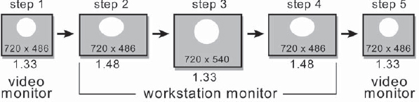
Figure 10-18: “Squaring” a Video Image on a Workstation

Step 1 shows the original video image displayed on a video monitor with non-square pixels. The aspect ratio of the image is 1.33 and the circle appears circular.

Step 2 shows the video frame transferred to the workstation monitor with square pixels. The image is the same size (720 × 486), but now has an aspect ratio of 1.48 due to the square pixels, and the circle is stretched horizontally by 10 percent, as is the entire image.

Step 3 shows the squared video frame on the workstation. The image size has been increased to 720 × 540 by stretching it in Y, the circle is once again circular, and the aspect ratio of the image is again 1.33. All transformations and blurs are done on this squared version.

Step 4 shows the squared image once again restored to its stretched form by resizing it back to 720 × 486, which is done after all filtering operations are completed. It is now ready to send to the DDR.

Step 5 shows the frame sent to the DDR and displayed on a video monitor. The non-square pixels of the video monitor squeeze the image 10 percent in X, restoring the circle to its proper shape and the image to a 1.33 aspect ratio.

This sequence of operations will restore the image to its correct aspect for filtering operations, but it is not without losses. Simply resizing an image from 720 × 486 to 720 × 540 and back will reduce its sharpness in Y a bit. This can't be helped.

10.4.3.2 Creating a New Image for Video

When you create an original image on your workstation with square pixels and then transfer it to video with squeezed pixels, the picture content will be squeezed 10 percent in X. Here is how to compensate. Start with the squared image size of 720 × 540 as shown in Step 3 of Figure 10-18. That is a 1.33 aspect ratio image with a width of 720. Create or place your image into this 720 × 540 image size. At this juncture, a circle will be a circle. After the image is completed, resize it to 720 × 486, as shown in Step 4. This will squeeze it in Y by 10 percent, introducing the 10 percent horizontal stretch. A circle will now look like it does in Step 4 when displayed on your workstation. Send this stretched version to the video monitor and the stretched circle will become squeezed to perfectly round again, as seen in Step 5.

Don't create a 640 × 486 image and then stretch it in X to 720. While mathematically correct, this stretches the picture data in X, which softens the image, degrading it. Creating it as a 720 × 540 and then squeezing in Y shrinks the image data, preserving sharpness.

10.4.3.3 PAL Pixels

PAL video suffers from the same non-square pixel issues, but the numbers are a bit different because the PAL pixel aspect ratio is 1.1 instead of NTSC's 0.9. This essentially reverses all of the stretch and size issues described in the previous section. When the image moves from video to the square pixels of the workstation the image appears stretched in Y instead of X, but the same blur and rotation issues still apply. To make a square version of a PAL frame, the original 720 × 576 frame is resized to 788 × 576.

10.4.4 Interlace Flicker

If you were to create a video frame on your workstation that consisted of a white square on a black background it would look fine on your workstation monitor. But when it was displayed on a video monitor you would suddenly notice that the top and bottom edges of the white square flickered. The reason for the flicker is that both the top and bottom edges of the white square consist of a white scan line adjacent to a black scan line. As the interlaced video fields alternate, the adjacent black and white scan lines take turns displaying, so the top and bottom edge flickers.

In the middle of the square each white line is adjacent to another white line, so they do not flicker as they “take turns.” The white square did not flicker on your workstation because its monitor uses a progressive scan instead of an interlaced scan. As we saw in Section 10.2.1.2, “Interlaced Fields,” interlaced scanning was developed specifically for broadcast television in order to lower the bandwidth of the transmitted picture. Interlace flicker is hardly ever an issue with live action scenes shot with cameras, because it is very difficult to get a perfectly straight high-contrast edge to line up exactly on the video field lines. If it does, then even a live action scene will exhibit interlace flicker.

When you create graphics of any kind on a workstation, however, they will invariably line up exactly on the scan lines. As a result, you stand a very good chance of introducing interlace flicker with any synthetic image, so it would be good to know how to prevent it. The fundamental cause is the two adjacent high-contrast scan lines, as in the white square. Knowing the cause suggests a solution—actually, two solutions. The first is to lower the contrast. Don't have a zero black scan line adjacent to a 100 percent white scan line. Perhaps a light gray and a dark gray would do, or two colors other than black and white.

The second solution is to soften the edges so that the hard white edge blends across a scan line or two to the black lines. If you don't want to run a light blur over the image, you could try repositioning the offending graphic half a scan line vertically. The natural pixel interpolation that occurs with a floating point translation might be just enough to quell your throbbing graphics.

And, of course, if your graphics package has a button labeled “anti-aliasing,” be sure to turn it on. Anti-aliasing is an operation that eliminates the jaggies in graphics. It calculates what percentage of each pixel is covered by the graphic element so that the pixel can be given an appropriate percentage of the element's color. For example, an 80 percent gray element that covers 50 percent of a pixel might end up making that pixel a 40 percent gray. Even with anti-aliasing, however, if your graphic element has a horizontal edge exactly lined up on a scan line it could end up with a hard edge and flicker like a banshee.

10.5 Working with Video in a Film Job

Perhaps you have a monitor insert in a feature film shot, or maybe you have to shoot the video out to film by itself. Either way, the idiosyncrasies of video will have to be coped with if there is to be any hope of getting good results. Video that originated on video will have to be handled differently than video that originated on film. How to compose to the film aperture with a 1.33 video frame that has non-square pixels is just some of the information in this section.

10.5.1 Best Video Formats

Very often the client will ask you what is the best video format to deliver to you for film work. The key issue in this is what format the video footage was originally captured on. Starting with video mastered on VHS and then dubbing it to D1 will not improve the quality of the video. It is amazing how many clients don't realize this until it is explained.

Having said that, the highest-quality video is D1. It is digital, component video, and uncompressed (except for that little half-res chrominance thing described in Section 10.2.1.5, “Color Resolution”). The next best is DigiBeta. It is digital, component video, but has a compression of about 2.5 to 1 (in addition to the chrominance thing). The compression causes some loss of picture detail, Sony's denials notwithstanding. This could be important when working with blue or green screens, since the loss of chrominance detail inherent in video is already hurting you. After that the next best is BetaSP. It is an analog format (bad), but it is component (good), but also has the 2.5 to 1 compression (bad). Nevertheless, it is a high-quality video source.

If the client has BetaSP, or any analog source, ask the client to make a digital dub (DigiBeta or D1) for you to import for the job. The main reason for doing this is that BetaSP is an analog tape, so settings on the front of the tape deck can alter the video levels affecting color and brightness. If the client makes a digital dub for you, the client will have made the color choices instead of you, and the video is read off the digital tape the same every time.

If the client's tape is D2, a digital composite format, it will not be as high quality as a D1 or DigiBeta, or perhaps even old analog BetaSP. Being a composite video format, the picture information has been compressed and encoded into the NTSC format, with a resulting loss of detail. It must go through a transcoder to convert it to component video, then the component video is converted to RGB for your workstation.

10.5.2 Video Mastered on Video

For video that was mastered (shot) on video, the frame rate is 30 fps and the frames will all be interlaced. For video to be incorporated into film, either as a monitor insert in a film effects shot or simply to transfer the video to film, it has to be de-interlaced and the frame rate reduced to 24 frames per second. How to de-interlace the video was covered in agonizing detail in Section 10.4.1, “De-Interlacing.” The speed change, however, has a couple of options.

After the video has been de-interlaced using your method of choice, frame averaging in your compositing software can be used to reduce the frame rate from 30 fps to 24 fps. This can look good if there is not too much motion in the picture (people dancing the jitterbug), or if the motion is not very high contrast (a white cat running through a coal bin). The frame averaging technique introduces cross-dissolved frames, which look like double exposures (because they are). This can become objectionable.

If the frame averaging does not work, another approach is to have the video transferred to PAL. The black boxes that do that have very elegant algorithms for averaging the video scan lines together and are much superior to simple frame averaging. This is not a flawless process and, depending on the black box used (there are a few to choose from) and the scene content, there can be artifacts. Testing the footage at a couple of conversion facilities might give you some good choices. The other issue with the PAL version is that it runs at 25 fps, not 24.

This is an easy one. Let the PAL video run at 24 fps with no speed change—one frame of video to one frame of film. It now simply runs 4 percent slow. This is the standard way PAL is transferred to film in Europe. No one can see a 4 percent slowdown, but you can hear it. The sound track must now be stretched 4 percent to stay in sync with the picture, but that is easy for the client to do. Make sure to mention this little audio detail to the client.

By far the best approach for a speed change from either 30 fps or 25 fps video frame rates to the 24 fps of film is with one of the new standards conversion boxes that use “motion compensation” algorithms. These systems actually do a motion analysis on each pixel to determine its motion from frame to frame, then create intermediate frames from this data. It is not frame averaging. They are literally shifting pixels to the position they would have had if the shutter had been open at the desired moment in time. Along the way, they can also convert the image to a progressive scan, which relieves you of the awful chore of de-interlacing and throwing away half of the picture information. They can even up-res the video to HiDef (1920 × 1080) if you want.

10.5.3 Video Mastered on Film

If the video was mastered (shot) on film and then transferred to video at 24 fps, there will be 3:2 pull-down frames to remove. This procedure was also discussed in arduous detail in Section 10.4.2, “The 3:2 Pull-Up.” Once the 3:2 pulldown is removed the video returns to the 24 fps speed of the original film, and you are good to go.

If the film was shot at 30 fps and transferred at 30 fps there will be no 3:2 pull-down frames, because one frame of film is on one frame of video. There is still the need for the speed change, of course.

10.5.4 Gamma Correction

As we learned in Chapter 9, “Gamma,” video comes with a built-in gamma correction of 2.2, making it quite “hot” (bright). Film is designed for a lower gamma, so a gamma correction will be required to make the video right for film. However, your particular production environment may include gamma corrected video transfers from the DDR to your workstation, then additional gamma corrections may be done to the images from your workstation to the film recorder. These are studio dependent setups, so it is not practical to offer any rules of thumb here. The best procedure may be simply to set your monitor for the proper display of film frames in your environment, then gamma correct the video to match. Use a gamma correction rather than a brightness operation because brightness operations scale the RGB values, and that is not what is needed.

10.5.5 Frame Size and Aspect Ratio

Let's say you have a 720 × 486 video image to somehow position into a film frame, while also correcting for the non-square video pixels. If the client wants the video to completely fill an academy aperture, which is common in a video to film transfer, simply resize the video frame to the academy aperture in one operation and you're done. Don't do it in two steps by first squaring the video to establish a 1.33 video frame, then resizing the 1.33 version up to film size. Each of those two operations introduces a filtering operation, softening the image each time. The image will be suffering from excessive softness as it is. A little image sharpening might be helpful on the film resolution frames, but this also increases noise and adds an edginess to the image if overdone.

The academy aperture has an aspect ratio of 1.37, which is close enough to the video aspect ratio of 1.33 to ignore. When the 720 × 486 video frame (which has an aspect ratio of 1.48 as seen on your workstation) is resized to academy it becomes a 1.33 image again just like on TV, correcting for the non-square pixels. The full frame of video fits nicely into the frame of film. But what if the video frame doesn't fit into the film frame so nicely?

If the mission is to fit the video footage into a film aperture of 1.85, for example, there are basically two choices, as shown in Figure 10-19. The entire video frame can be fitted from top to bottom in a 1.33 “window” within the 1.85 format, but there will be the black “curtains” on either side. The advantages are that the image is sharper and you get to keep the entire picture, but the black curtains may be objectionable. The other alternative is to crop the video frame to 1.85 and fill the entire film frame. The problems with this format are that the increased size results in a much softer image than the fit format, and the original picture content is now seriously cropped. The 1.33 video frames are composed (framed) more tightly than 1.85 film frames, and cropping video like this can sometimes result in seeing only a pair of eyes and a nose instead of a face. Be sure to discuss these two composition options with the client. It is amazing how many of them will be totally surprised to discover that they must choose between these two options (or perhaps an in-between compromise).

10.5.6 Cropping Non-Square Pixel Frames

If it is necessary to crop the video frame to fit a film aperture, it would be most elegant to make a single crop and a single resize to the target size. This will avoid multiple scaling operations and the increased softening that they introduce. It takes a little extra figuring to make a correct crop that compensates for the non-square pixels of a 720 × 486 video frame, but the following procedure will help. The example given is for a 1.85 film aperture.

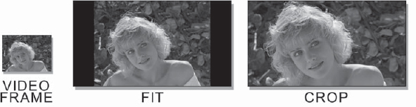
Figure 10-19: Alternative 1.85 Film Compositions for Video Frames

Step 1: Calculate the width of an exact 4:3 (1.33) aspect ratio version of the image based on the number of scan lines. The number of scan lines times the aspect ratio gives you the width: 486 × 1.3333 = 648 pixels wide, so the 1.33 version is 648 × 486.

Step 2: Calculate the height you need for a 1.85 crop of this 1.33 version (648 × 486) of the image. The image width divided by the aspect ratio gives you the height: 648 ÷ 1.85 = 350 scan lines high.

Step 3: Crop the 350 scan lines out of the original 720 × 486 video frame. A 720 × 350 crop is not a 1.85 image, but is in fact a 2.06 aspect ratio (720 ÷ 350 = 2.06 aspect ratio). However, when the 720 × 350 image is resized to the 1.85 film aperture, it will square up the image. In other words, we have cropped a single window out of the 720 × 486 video frame, which will compensate for the non-square pixels when it is resized to 1.85.

This procedure also works for the 720 × 576 PAL frames, with minor modifications. For Step 1, the 1.33 aspect ratio calculation results in a frame size of (576 × 1.3333 = ) 768 × 576. For Step 2, you still calculate how many scan lines are needed for 1.85, but you are using the longer PAL scan line of 768 pixels (768 ÷ 1.85 = 415 scan lines). For Step 3 you would crop 415 scan lines out of the original 720 × 576 PAL image, then resize it to the 1.85 film aperture.

10.6 Working with Film in a Video Job

If you have frames of scanned film to incorporate into video, several operations must be performed on the film scans. The film frame aspect ratio will have to match the video, non-square pixels will have to be introduced, the frame size will have to be reduced, and the film speed will have to be changed. Following are the steps for preparing film frames to be used in a video format. Be sure to use a gamma correction, not a brightness operation, to raise the brightness of the film frames up to video levels.

Step 1: Calculate the target video image height. Using the 1.33 form of the video frame calculated previously (648 × 486 for NTSC, 768 × 576 for PAL), calculate the needed height of the video image using the image width divided by the desired aspect ratio. For full frame video the aspect ratio is 1.33, so the height is (648 ÷ 1.33 = ) 486, as expected for a full frame of video. For a 1.85 letterbox format, the height becomes (648 ÷ 1.85 = ) 350.

Step 2: Calculate the target video frame size. Using the width of 720 for an NTSC video frame, the full frame version becomes, unsurprisingly, 720 × 486. The 1.85 letterbox version becomes 720 × 350.

Step 3: Crop a window out of the film frame that matches the target aspect ratio for the video. For full frame video, crop a 1.33 window from the film. For a 1.85 letter-box, crop a 1.85 window. This cropped window could be the full size of the film frame, or some portion thereof. It matters not.

Step 4: Resize the window cropped from the film down to the target video frame size calculated at Step 2. For full frame video, the film crop destination size is 720 × 486. For the 1.85 letterbox it is 720 × 350.

Step 5: Pad the video frame out to 486 scan lines, if needed. If it is a full frame video, then you already have 486 scan lines. For the 1.85 letterbox, you need to pad (486 – 350 = ) 136 scan lines. Pad half this number of scan lines above the image and half below.

Step 6: Speed change the film to video frame rates. The fastest and easiest way to do this is to let the DDR do it. Send the video-sized film frames to the DDR, then set the DDR to play them back with a 3:2 pull-down as they are laid off to videotape. If your DDR does not have this “cine” feature, then you will have to introduce the 3:2 pull-down with your compositing software as you write the frames to disk, then send the cine-expanded frames to the DDR for layoff to videotape. Failing both of those, it is entirely possible, if not highly painful, to create your own cine-expand operation within your software using the information in Section 10.3.1, “The 3:2 Pulldown.”

10.7 Working with CGI in a Video Job

Ideally, your cgi rendering software will offer you the options for an interlaced 30 fps 720 × 486 image with a pixel aspect ratio of 0.9 and a gamma of 1.0. Any cgi package worth its weight in polygons will at least offer the correct frame rate and frame size. If anything is missing it will probably be the interlacing and the pixel aspect ratio options.

Rendering on fields and interlacing may be helpful if there is extremely rapid motion in the action. Usually good motion blur and a 30 fps render are just fine. Some folks actually prefer the look of a 24 fps render that is cine-expanded. They feel it makes the cgi look more “filmic.”

If your rendering software does not offer a non-square pixel aspect ratio option, you will have to render a 1.33 image and then resize it. For NTSC, render a 720 × 540 and resize to 720 × 486. For PAL, render a 788 × 576 and resize to 720 × 576. Squeezing the rendered frames like this distorts the anti-aliasing a bit compared to rendering the frames with the correct aspect ratio pixels. If this becomes a visible problem, try increasing the anti-alias sampling.