

There are many ways to combine images by using image blending operations rather than a composite. These operations have the virtue of not requiring a matte, which is a huge advantage because creating a matte is often a difficult and time-consuming process. Two images are input to an image blending operation and its output is the new image. It’s as simple as that. Image blending is also the core technology behind speed changes, a phenomenon that is growing in demand. While these operations have been seen earlier in the context of working with mattes, in this chapter the focus is on how they are used to blend two color images together for an artistic treatment.
The two keys to working with image blending operations are knowing when to use which one and how to control them. This chapter covers both topics. Each image blending operation has a section describing when to use it as well as tips on how to adjust the appearance of the blended image and a production case study. Most of the image blending operations also have “no-change” colors that you can take advantage of to limit the effects of the image blending to just the parts of the picture you want.
Homage is paid to Adobe Photoshop image blending modes because of Photoshop’s enormous contribution to the entire visual effects industry and its application to our work in digital compositing. We are all Adobe Photoshop users and many readers will want to relate what they read here to Photoshop. All of these image blending operations are found in Photoshop, and most of them are found in the Photoshop Layers blending modes. For those not found in the Layers blending modes their secret locations are revealed.
7.1 THE MIX OPERATION
We start our tour of image blending with the ubiquitous and humble mix operation. The mix is used whenever you want to “super” (superimpose) one image over another in such a way that both images are still visible, like the examples in Figure 7-1 through Figure 7-3. A mix is performed internally by first darkening the A and B images and then adding them together. The amount of darkening for each image is reciprocal, which means, for example, if one image is darkened by 25% the other is darkened 75% so that their darkening adds up to 100%. A slider or percentage number will be available so the amount of the mix can be adjusted to taste. In Photoshop the mix operation would be equivalent to the Layer Opacity setting.
Figure 7-1 Image A
Figure 7-2 Image B
Figure 7-3 Mix of A and B
The mix is the image blending operation used to do a dissolve. A dissolve is just a mix operation where the amount of mix is animated over time. The mission is to transition from image A to image B in gradual steps over time like the example in Figure 7-4. The sequence starts with image A at 100%, then image A fades down as image B fades up, ending with image B at 100%. The dissolve is the process of transitioning from image A to image B. The mix is the mathematical operation performed at each frame to achieve the dissolve.
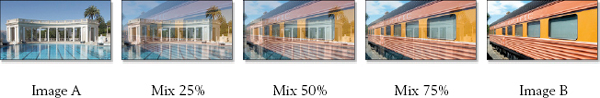
Figure 7-4 The mix operation performs the dissolve between two images
The pixel behavior of the mix operation can be seen in Figure 7-5. The horizontal and vertical bars images have five bars each ranging from zero black to 100% white. They have been blended together with the mix operation set to 50% to produce the “Mixed” image. Any pixel in the Mixed image can be traced back to the horizontal row and vertical column that it was made from to see the effect of blending them at 50%. This illustration shows all of the cross-combinations of mixing light pixels with dark, dark with dark, light with light, etc.
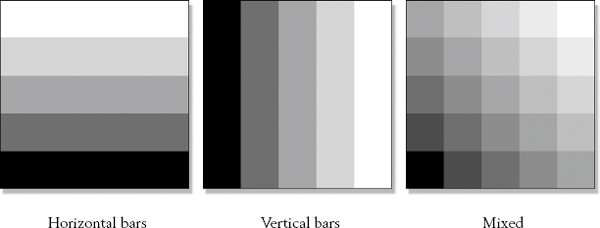
Figure 7-5 Pixel behavior of the mix operation
The multiply operation simply multiplies two images together on a pixel-by-pixel basis. The visual results are analogous to putting the source image in a slide projector and projecting it onto an object in the target image. This technique is the solution for all those shots where a character or object moves in front of a projector. It is also useful when you want to paint the source image onto the target image while retaining some of the color and detail of the target image, as if it were stained. Photoshop supports the multiply operation. Perhaps you have wondered what it might be used for.
The case study for the multiply operation is a television commercial for a shameless floral company that wishes to besmirch the natural beauty of Yosemite’s El Capitan (Figure 7-6) with crass commercialism by projecting their flower product (Figure 7-7) onto its majestic face. Sometimes, as professionals, we even have to work on hemorrhoid commercials. The prepped flower is shown in Figure 7-8 with a white surround, which is multiplied by the El Capitan image to produce the final results in Figure 7-9.
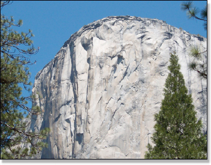
Figure 7-6 El Capitan
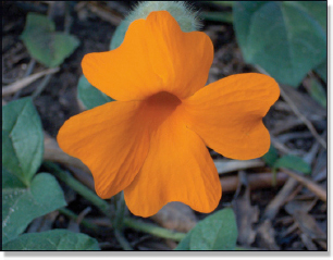
Figure 7-7 Flower
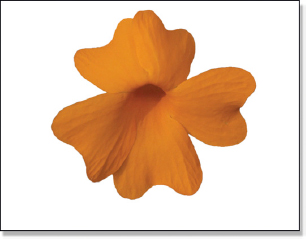
Figure 7-8 Prepped flower
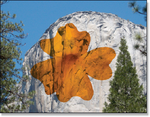
Figure 7-9 Multiplied flower
The prepped flower has a white surround because white is the “no-change” color for the multiply operation. Any pixel multiplied by white (one) is always the original pixel. When any two pixels are multiplied together the results are always darker than either of the original pixels. Why this is so will be demonstrated below. In the meantime, this means that the projected image may need to be brightened up for the multiplied results to look right. This may also mean that both images might need to be promoted to 16 bits prior to the multiply so they will tolerate the brightening without introducing banding.
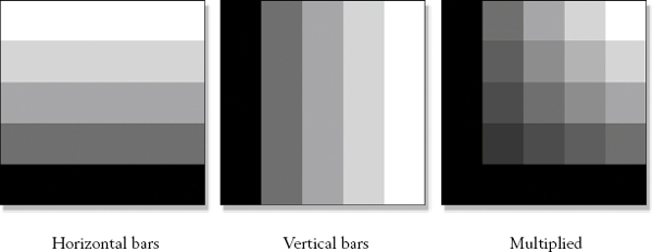
Figure 7-10 Pixel behavior of the multiply operation
The pixel behavior of the multiply operation is cunningly revealed in Figure 7-10. The two bars images have been multiplied together to produce the “Multiplied” image. It shows all of the possible cross-combinations of multiplying dark and light pixels—for these five shades of gray, anyway. As we might expect of a multiply operation, any black in either image produces black in the multiplied image. What may not be expected is that in the multiplied image the pixels are darker than their source pixels.
To see why this is so, consider two pixels with a value of 0.4 and 0.6, for example. When multiplied together the result is 0.24 (0.4 × 0.6), a result that is darker than either original pixel. Any pixel in the Multiplied image can be traced back to the horizontal row and vertical column that it was made from to confirm the darkening effect of multiplying them together.
7.3 THE SCREEN OPERATION
The screen operation is one of the most powerful and useful of the image blending operations because it solves a very common problem in digital compositing, and that is to add light rays to a shot. Glows around lights, laser beams, God rays, and flashlight beams are just a few of the many applications for the screen operation. All you do is prepare the “light layer” element then screen it with the background. No mattes, no fuss, and, most importantly, no clipping. Photoshop has this operation and uses the same name.
Our case study for the screen operation is a television commercial designed to grant a heavenly aura to the banal Las Vegas gambling casino pictured in Figure 7-11. Such is the power of the screen operation. The art department has prepared the plate of God rays shown in Figure 7-12. Areas of the picture that we do not want to change are made zero black in the God ray plate because black is the no-change color for the screen operation. The God rays are screened with the background and the results shown in Figure 7-13.
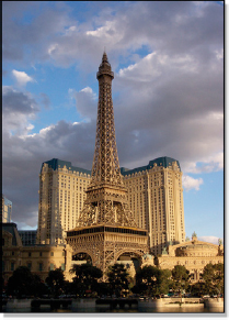
Figure 7-11 Background
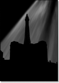
Figure 7-12 God rays
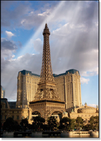
Figure 7-13 God rays screened
The reason that the screen operation is such an excellent simulation of light beams is that, like real beams of light, they do not block or obstruct the background image like a composite would. A semi-transparent composite would actually first darken the background pixels, and then add in the light. This causes a loss of detail in the background lowering its contrast and flattening it out. The screen operation adds the light without obscuring the background just like real beams of light. It can even be used to add atmospherics to a shot such as smoke or dust when they are photographed over black and have no matte.
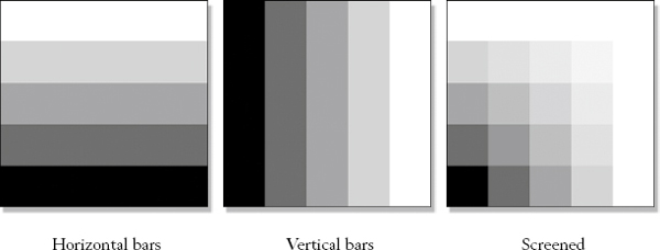
Figure 7-14 Pixel behavior of the screen operation
The secrets of the screen operation’s pixel behavior are revealed in Figure 7-14. The two bars images have been screened together to produce the “Screened” image which shows all of the possible cross-combinations of screening dark and light pixels. Comparing it with the Multiply results in Figure 7-10 above, you can see why the screen operation is considered an inverted multiply. With the multiply operation, if either pixel is black the results are black. With the screen operation, if either pixel is white the results are white. Also, with the screen operation the pixels are lighter than their source pixels, but with the multiply operation they are darker.
7.4 THE MAXIMUM OPERATION
When two images are “max’d” (maximumed) together the computer compares them pixel by pixel and simply uses whichever pixel has the greater value in the output image. This can be a useful operation for lifting a light colored element out of one plate and merging it into another. This is especially useful when the item of interest is on a gradient rather than a smooth uniform surface, which seems to be the case with many real-world pictures. The rules are that the light colored element must be surrounded by a darker color and the destination plate must have a similar dark color. This actually happens more often than you might think. Photoshop offers this operation but calls it lighten rather than maximum. Perhaps they call it lighten because the resulting image retains the lightest pixels of each image.
The case study of the maximum operation is the classic Victorian house in Figure 7-15. Previous shots of the house had clouds in the sky, but on this day Mother Nature was uncooperative. The mission is to lift the clouds from the shot in Figure 7-16 and place them over the house. Figure 7-18 shows the prepped cloud plate. The cloud layer was first color corrected to approximate the blue sky color in the original plate then masked with black. This prepped cloud plate was then max’d with the original plate to produce the results in Figure 7-17.
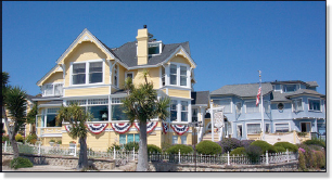
Figure 7-15 Original plate
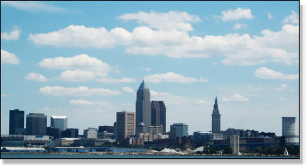
Figure 7-16 Clouds to be lifted
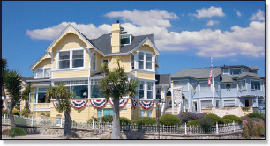
Figure 7-17 Max’d clouds
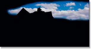
Figure 7-18 Prepped clouds
The clouds were prepped with a black surround because black is the no-change color for the maximum operation. Any pixel max’d with black will always result in the original pixel. The virtue of maxing the layers together rather than a composite with a matte is that the maximum operation feathers in the clouds without a matte line. Because the gradients of the two skies are slightly different a matte line would have been unavoidable. The prepped clouds’ blue sky was also color corrected to closely match the target plate because the maximum operation is done on a channel-bychannel basis so all three channels must be close to the target.
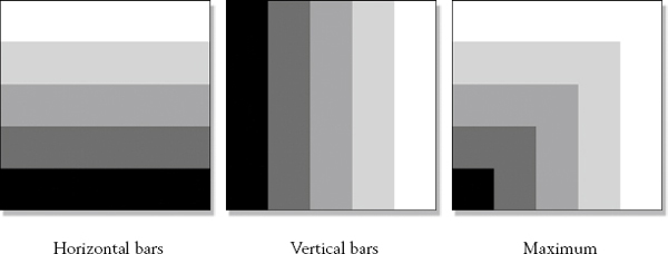
Figure 7-19 Pixel behavior of the maximum operation
The results of the maximum operation are shown in Figure 7-19. The brightest pixel value from either image has been retained in the “Maximum” image.
7.5 THE MINIMUM OPERATION
The minimum operation is conceptually identical to the maximum operation, only different. The computer compares the two images on a pixel-by-pixel basis and then uses whichever pixel is the minimum value in the output image. This can be useful for lifting dark elements out of one plate and placing them in another. The rules here are that the object of interest must be dark and surrounded by a fairly uniform lighter color. The target image must also have a similar light color. Keep in mind that the source image can be color corrected to get the surround colors similar. Photoshop offers this operation but calls it darken rather than minimum, probably because the resulting image keeps the darker pixels from the two source images.
The case study for the minimum operation starts with the original plate in Figure 7-20. The frenzied director wanted the lighthouse dramatically framed by the sun when the Goodyear blimp flew by. Delayed by a headwind, the blimp was late and the sun had dipped too low by the time the blimp lumbered by in Figure 7-21. The blimp must be lifted out of Figure 7-21 and seamlessly placed in the original plate. The blimp plate is prepped with a white surround in Figure 7-22 and then min’d with the original plate to produce the dramatic shot in Figure 7-23. The director was thrilled. Shot saved, hero compositor.
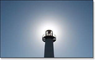
Figure 7-20 Original plate
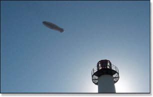
Figure 7-21 Blimp to be lifted
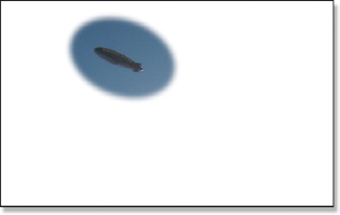
Figure 7-22 Prepped blimp
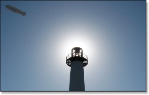
Figure 7-23 Min’d blimp
The blimp was prepped with a white surround because white is the no-change color for the minimum operation. Any pixel min’d with white will always result in the original pixel. Again, the minimum operation blended the blimp without any of the matte lines that a composite would have produced, plus it was quick and easy to create the prepped blimp plate with a simple soft-edge mask even though the blimp was moving.
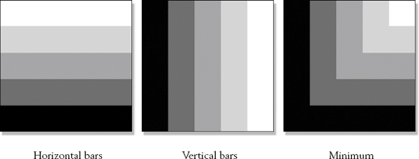
Figure 7-24 Pixel behavior of the minimum operation
The minimum operation is shown in Figure 7-24. The darkest pixel from either image has been retained in the “Minimum” image.
7.6 THE ADD OPERATION
The add operation, not surprisingly, simply adds two images together on a pixel-bypixel basis. Similar in look to the screen operation, the add operation is also good for adding atmospherics and other subtle detail to a shot. The add operation can give the atmospheric element more “presence” in the shot than the screen operation, but there is a danger of introducing clipping. In Photoshop the Add operation is not found in the Layers blending modes but in the Image > Apply Image as well as in the Image > Calculations.
The case study for the add operation starts with the night buildings in Figure 7-25. A creepy atmosphere is needed for a cheesy detective movie, so the fog layer from Figure 7-26 needs to be added. The fog was shot on a black screen, so the only preparation was to lower the black level so it does not milk up the blacks in the finished picture shown in Figure 7-27.
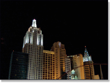
Figure 7-25 Original plate
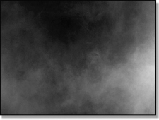
Figure 7-26 Fog
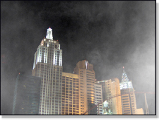
Figure 7-27 Fog added
The no-change color for the add operation is black since adding black (zero) to any pixel always results in the original pixel value. As mentioned above, the add operation is dangerous to use because it can introduce clipped pixels. If a pixel in the fog plate with a value of 100 is added to a pixel in the original plate with a value of 200, the results will obviously be 300. However, the computer will clip the 300 to 255 because that is the maximum value allowed. Always check for clipped pixels when using the add operation. In fact, this operation is so dangerous that Photoshop hides it in the Image > Apply Image and the Image > Calculations menus.
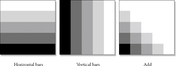
Figure 7-28 Pixel behavior of the add operation
The add operation results are shown in Figure 7-28. The pixel values from the two bars images have been summed together in the “Add” image, but over half of them are pure white. This is because their totals exceed 255 so they are all clipped.
(Download www.compositingVFX.com/CH07/Horizontal bars.tif and Vertical bars.tif to try these image blending operations on your workstation.)
7.7 THE SUBTRACT OPERATION
The subtract operation does exactly what you would expect—subtract one image from another. While very useful for the internal workings of advanced keying operations such as matte extraction and despill, it is not particularly useful for the type of image blending applications that we are discussing here. Perhaps this is why Photoshop buries the subtract operation in the Image > Apply Image and the Image > Calculations menus.
7.8 NO-CHANGE SUMMARY TABLE
All of the image blending operations listed above except for mix have a nochange color that you can use to prevent areas of one image from affecting the other. Table 7-1 is a summary list of each operation and its associated no-change color for handy reference.
7.9 ADOBE PHOTOSHOP BLENDING MODES
Adobe Photoshop has a long list of image blending modes in the Layers palette that include all that we have seen here (except they call maximum “lighten” and minimum “darken”) plus many more. The other Photoshop blending modes, such as “Overlay,” “Soft Light,” and “Hard Light,” use complex mathematical equations to perform their blending operations. Some digital compositing programs can duplicate Photoshop blending modes, and others cannot. And herein lies a trap.
Table 7-1 No-change color summary
| Operation | No-change color |
|---|---|
| Mix | None |
| Screen | Black |
| Maximum | Black |
| Minimum | White |
| Multiply | White |
| Add | Black |
| Subtract | Black |
If the art director does a “pre-viz” (pre-visualization) of a shot for the client using one or more of these exotic Photoshop blending modes, the client will reasonably expect the final composite to look the same. The problem here is that if the compositing program does not support the Photoshop blending modes that the art director used to create the pre-viz version then the compositor may not be able to deliver a matching shot. The hapless compositor will be forced to spend a great deal of time in a frustrating attempt to match the look of the pre-viz. In the end, after a great deal of work, the results might be close, but they will never be an exact match. The bottom line is that the art director must not use image blending operations for a pre-viz that cannot be duplicated by the compositors.
7.10 SPEED CHANGES
A very important class of image blending operations is speed changes. A shot might be 115 frames long and it needs to be shortened to 97 frames to fit the cut. Or perhaps the actor was too quick in his furtive glance so the director wants it slowed down for dramatic impact. The demand for this effect is skyrocketing because of the growing tendency to edit feature films with off-line editing systems as if they were an MTV show with lots of fancy editorial effects, including speed changes. Think of it as job security for us compositors.
When a shot is lengthened or shortened some method must be used for generating the in-between frames. There are three different image blending techniques that one might choose from, each with its own advantages and disadvantages. Following is a description of each one, their relative strengths and weaknesses, and when to use them.
7.10.1 Skip Print/Frame Duplication
The simplest of all speed changes is to simply drop frames out of the shot. If every other frame is dropped the shot is half as long and the action twice as fast. Ugly, but easy. In movieland this is referred to as a skip print, but each compositing program has its own terminology for this. To lengthen a shot, frames may be duplicated. This would be the frame duplication method. There is no attempt to make an in-between frame, so these two methods can be lumped together and referred to as integer (whole number) speed changes.
Of course, in the real world your speed change shots will rarely be exactly double or half the speed. More often it will be like the example above where you need to take 115 frames down to 97. That’s an awkward 15.65% speedup in the shot requiring that you drop 18 frames out of the shot. To drop 18 frames out of 115 means you need to drop one frame every 6.38 frames. There is no frame 6.38, only frame 6 or frame 7, so the computer simply drops the frame nearest to 6.38. Not much of an image blending strategy. This, unfortunately, is the only option with an integer speed change.
There are two main problems with integer speed changes. The first is that because the correct in-between frames are not used the action can look odd to the eye. It can stutter or clatter across the screen. The second problem is that the motion blur will not be correct for the new speed. If the action is sped up the motion blur will be insufficient and can introduce motion strobing—where the motion takes on a staccato-like jitter. If the shot is slowed down the motion blur can be excessive resulting in a blurry looking shot. Keeping the motion blur correct for a speed change shot is a very important issue.
7.10.2 Frame Averaging
One step up from the integer speed change is frame averaging, but it is a small step up. With this method the computer actually makes an in-between frame to smooth out the action and avoid the stutters and judders of the integer method. It also helps with the motion blur problem (sort of). Frame averaging does pretty much what its name implies—it averages adjacent frames together over the length of the shot using the mix operation we saw earlier. This results in a shot with a series of cross-dissolves like the example in Figure 7-29.

Figure 7-29 Frame averaging uses cross-dissolves
Frame 1 and frame 2 in Figure 7-29 are original frames from the shot and we need to make frame 1.5 exactly halfway in between. Using a mix operation set to 50% we get the averaged frame in the middle. If our speed change needed a frame 1.2 we would mix 80% of frame 1 and 20% of frame 2. The 15.65% speed change in the integer example above is now trivial for the computer using frame averaging. It just calculates what mix percentages are needed for each new frame and then mixes them accordingly, creating a “rolling cross-dissolve” to produce the new shot. Mixing the frames like this even introduces a pseudo motion blur.
Table 7-2 shows how the frame average rolling cross-dissolve is calculated to stretch a 10-frame shot into a 14-frame shot. The top row shows the new output frame numbers and the bottom row is the frame average values calculated for each frame. The original frame 1 should be used in tact as frame 1 of the new shot and frame 10 should also be used in tact as frame 14, but each of the in-between frames is some averaged floating-point value. Frame number 5, for example, calculated a frame average of “3.8” from the original clip, which means it will do an 80% mix of frame 3 with frame 4. Similarly, frame number 13 calculated a frame average of “9.3” resulting in a 30% mix of frame 9 with frame 10.
Table 7-2 Frame averaging 10 frames to 14 frames

This sounds pretty good and works fairly well if the action in the shot is not very quick or the camera move is not very fast. If a shot is slowed down (stretched) and there is fast action, the frame averaged shot looks “dissolvey” because, well, it is. As we saw above, if you used an integer speed change on a fast action shot it would look “strobey.” Is there nothing that can be done to speed change a fast action shot?
7.10.3 Optical Flow
The answer to the nagging question of how to speed change a fast action shot is optical flow. Also known as motion vector or motion analysis, optical flow is another of those wondrous things that only a computer can do. The concept is that the computer compares two adjacent frames and creates a list describing how small groups of pixels have moved from the first to the second frame. One small group of pixels moved to the right a bit. Another small group moved down a bit. And so it goes over the entire frame. To describe the motion of each pixel group the computer uses a little mathematical “arrow,” called a vector. The length of the vector records how far the pixels moved and its orientation indicates the direction of movement.
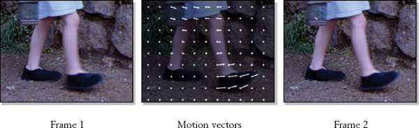
Figure 7-30 Optical flow uses motion vectors
Figure 7-30 offers a simplified illustration of the motion vectors in optical flow. After comparing small pixel groups in frame 1 to frame 2, the computer decides how far and in what direction each group moved to create the motion vectors. The white dots indicate a region that did not move at all. The regions with vectors that had movement are indicated by the direction of the arrow and the arrow lengths indicate how far they moved. Note that the region where the foot is moving a lot has long vectors, while the lantern and shirt only moved a little so have short vectors.
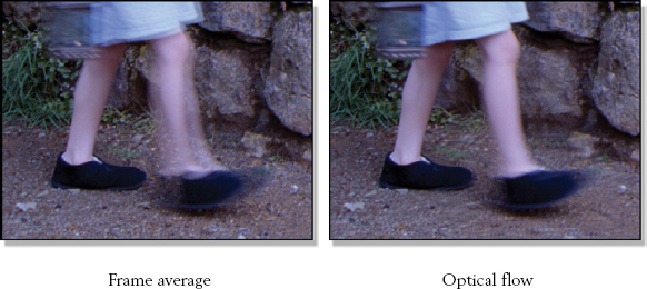
Figure 7-31 Comparison of frame average and optical flow for frame 1.5
Once we have the motion vectors for frame 1 to frame 2, it is now possible to synthesize a much more realistic in-between frame. Suppose we need frame 1.5. The computer shifts the pixels from frame 1 by half the distance of the motion vectors and creates an “honest” frame 1.5. The visual results of using the motion vectors to generate a new frame are vastly superior to a simple frame average. Just compare the exact same frame 1.5 in Figure 7-31 created with frame averaging and optical flow. The frame averaged version appears as exactly what it is—a 50% mix of frames 1 and 2. The optical flow version, however, is a “synthesized” frame using the motion vector information from the optical flow calculations.
One key advantage of optical flow is that once the motion vectors are generated they can be used to create any arbitrary fractional frame between frames 1 and 2, such as frame 1.2, frame 1.8715, or anything at all. Figure 7-32 shows a sequence of actual optical flow interpolated frames between the same frame 1 and frame 2 used above. The interpolated frames represent where the action should be on frames 1.25, 1.5, and 1.75. This technology can even be used to completely replace a destroyed frame. If frame 5 is lost, just use optical flow to interpolate a new frame between frames 4 and 6. Optical flow is truly wondrous.
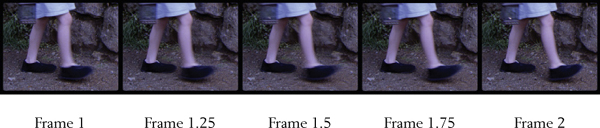
Figure 7-32 Speed change with optical flow
But wait—there’s more! Another key advantage of optical flow technology is that it can also change the shutter timing of a shot. If a shot were seriously shortened then the motion blur in the original frames would be insufficient for the shorter version and could introduce motion strobing. Conversely, if a shot is seriously extended then the original motion blur could be excessive, making the shot look soft and smeared. Most optical flow programs offer an option to change the shutter timing, which in turn alters the motion blur of the retimed shot.
So that was the good news. Now for the bad news. Optical flow is a spectacular solution to the speed change problem, BUT—and this is a very big but—it frequently also introduces artifacts that have to be fixed. Optical flow programs (and there are several available) are not flawless and can get confused under certain conditions. Those conditions vary from brand to brand, but they are all vulnerable. When this happens it can be major surgery to repair the artifacts, which might require elaborate techniques akin to wire and rig removal. While this is time-consuming and can drive up costs and schedules, the results of optical flow are well worth it.