
Before we get into the really cool stuff about compositing visual effects shots, we first need to develop some key concepts and bulk up our vocabulary. While digital imaging is a very technical subject, we will explore it here with less tech and more illustrations. The key concepts can be understood without binary math or quadratic equations with the help of some carefully crafted explanations. A detailed account of digital imaging would in fact be a whole other book in itself. In fact, there are many such books available. Once you have a foundation in digital imaging basics on a conceptual level from this book you can then comfortably move on to more advanced books on the subject. One that leaps to mind is Digital Compositing for Film and Video by Steve Wright.
The first topic in this chapter is the structure of digital images. That is, how pictures on a monitor, digital projector, or film are represented inside the computer. This is essential information because this is what the digital compositor actually works with. We then take a look at key attributes of digital images that affect manipulating them with a computer such as resolution, aspect ratio, and bit depth. All of the images that we work with must come from and go to some kind of file format, from which there is a confusing array to choose. There is a special section on just the key file formats that you will likely need to work with and a neat little summary of when to use which one. Very useful stuff if you ever plan to save an image to disk.
2.1 STRUCTURE OF DIGITAL IMAGES
Digital images have a “structure”—that is they are built up of basic elements that are assembled in particular ways to make a digital image. The basic unit of a digital image is the pixel, and these pixels are arranged into arrays and those arrays into one or more layers. Here we take a tour of those pixels, arrays, and layers to see how they make up a digital image.
Digital images are divided into little “tiles” of individual color called pixels*. This is necessary for the computer to be able to access each one individually in order to manipulate it. Each pixel is also filled with one solid color. When the pixels are small enough they blend together to form a smooth image to the eye, like the example of Marcie, Kodak’s famous film girl seen in Figure 2-1. However, if you move closer than the normal viewing distance you might start to see her pixels, as in Figure 2-2. If you get way too close you can clearly see her pixels in Figure 2-3.
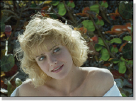
Figure 2-1 Marcie
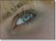
Figure 2-2 Close up
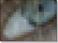
Figure 2-3 Marcie’s pixels
Pixels have two attributes essential to the computer. First, they are organized in neat little rows and columns like a checkerboard, and in computerland this is called an array. Having the pixels arranged into an array like this is essential for the computer to be able to locate them. The horizontal position of a pixel in an array is referred to as its position in “X” (the classic horizontal direction) and its vertical position is referred to as “Y” (the classic vertical direction). This gives each pixel a unique location, or “address,” in X and Y. For example, if you had an image that was 100 pixels wide and 100 pixels tall, you could identify the exact location of a specific pixel by saying it was 50 columns over (50 in X) and 10 rows down (10 in Y). Shorthand for this is to say its XY location is 50,10. This pixel would be distinct from its neighbor that was located one column to the right at 51,10 or in the row below at 50,11. In fact, each pixel would have a unique XY location in the image and could be addressed by the computer that way. Which it is.
The other key attribute that a pixel has is its single color. By definition, a pixel is all one solid color. Color variations or textures are not allowed within a pixel. The color of each pixel is represented by a number. In fact, pixels are simply sets of numbers that represent colors that are arranged in neat rows and columns. They don’t become a picture until those numbers are turned into colors by a display device such as a TV set or computer monitor.
2.1.2 Grayscale Images
Grayscale images are known by many names, such as black and white images, one-channel images, and monochrome (one color) images. The variety of names is due to the fact that several different technical disciplines have developed their own terms to describe the same thing. This happens a lot in computer graphics because it historically merges many disciplines. For purposes of clarity and brevity, I will refer to them here as grayscale images. Grayscale images are very common in computer graphics and due to their simplicity they are a nice way to gently approach the topic of digital images. They have only one channel, or layer, while color images have three channels or more, which we will see shortly.
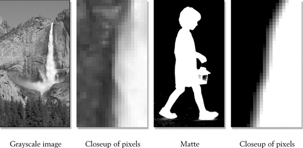
Figure 2-4 Examples of grayscale images and their pixels
An example of a grayscale image is digitizing a black and white photograph, but another, perhaps more pervasive, example are all of the mattes in the world. Mattes are used to composite one image over another. These two examples are illustrated in Figure 2-4. They are both grayscale images, so they have no color. While the two examples appear quite different, the one thing they have in common is that they are both one-channel images. That is to say, they have one channel, or layer, that is made up of just one array of pixels with brightness values ranging from black to white and shades of gray.
(To view high resolution versions see www.compositingVFX.com/CH02/Figure 2-4 grayscale.tif and Figure 2-4 matte.tif)
To witness this one channel array of pixel values up close and personal, Figure 2-5 zooms into a tiny region of pixels in the grayscale image of Figure 2-4. The numbers in Figure 2-5 are the code values of each pixel. They are called code values because their numerical values encode, or quantify, the brightness of each pixel. The gray chip that each code value sits on represents how bright that pixel will appear when displayed on a monitor. These code values are organized into the array that the computer uses internally to represent the picture. The key points here are that there is only one array of code values—it is called a channel—and the code values represent only a brightness, not a color.
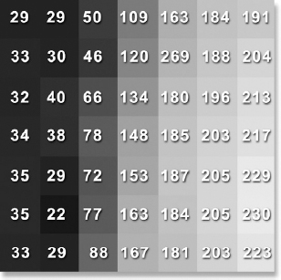
Figure 2-5 An array of pixels
2.1.3 Color Images
The human eye appears to see a full spectrum of color in the real world, but is actually only sensitive to red, green, and blue wavelengths of light. We get all of the in-between colors because the brain “mixes” portions of red and green, for example, to get yellow. The same trick is used in all of our image display devices such as television, flat panel displays, digital projectors, and feature film. These display devices actually only project red, green, and blue colors, which our brains cheerfully integrate into all of the colors of the rainbow. To make a color display device for humans, then, all you need is red, green, and blue, which is abbreviated to RGB.
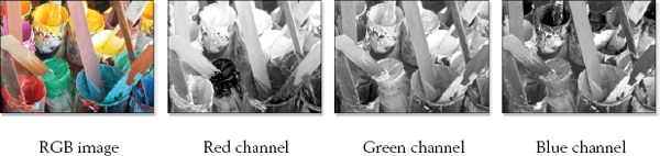
Figure 2-6 An RGB image is made of up three channels
Digital images that need to convey color to human eyes obviously must have RGB data in them. In the previous section we saw how a grayscale image has only one channel and it is made up of a single array of numbers to represent brightness values from black to white.
However, if we use three of these channels we can assign one channel to red, one to green, and the other to blue. This scheme will allow us to assign a unique RGB code value to each pixel in our color image by putting different code values in the red, green, and blue channels of each color pixel. We now have a color image composed of three channels, which is referred to as an RGB image, illustrated in Figure 2-6. Note how the yellow paint cans in the RGB image appear bright in the red channel, medium in the green channel, and dark in the blue channel. Having these different values in each channel is what gives the image its colors.
The odd thing about the RGB image is that while the data in each channel represents the values of the red, green, and blue colors on a pixel-by-pixel basis, the data itself in each channel is various shades of gray. It is different shades of gray because the data actually represents the amount of brightness of that channel for each pixel. This is what Figure 2-7 illustrates.

Figure 2-7 Gray RGB data becomes color
Consider the red pixel on the left in Figure 2-7. The three gray RGB chips above it create the red pixel and you can see how the R (red) chip is very bright, while the G (green) and B (blue) chips are very dark. If you have lots of red and very little green and blue that means you have red. The yellow pixel next to the red has bright R and G values above it, but a low (dark) B value, which is the quintessential definition of yellow. The skin tone chip shows a more typical RGB combination to make a common skin tone color. The gray pixel on the end shows a special case. If all three of the RGB values are the same it produces gray. In fact, that is the definition of gray—all three channels having equal values of brightness. When the RGB values of a pixel are different from each other we get color.
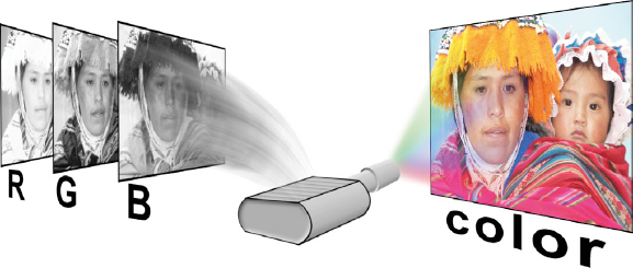
Figure 2-8 Gray RGB data gets its color from the display device
So if the RGB data is actually gray, where does the color come from? The color comes from the display device itself (television, digital projector, etc.) as illustrated in Figure 2-8. The gray data for the red channel, for example, is fed to the red lamp of the digital projector, which fills the entire screen with the appropriate amount of red light at each pixel. The green and blue data go to their respective lamps. The red, green, and blue images on the screen are superimposed over each other and the eye sees—color! The key point to walk away with is that a color image is a three-channel image that contains separate RGB data in each channel, and the data in these channels is, in fact, gray.
Adobe Photoshop can handily illustrate this point. Load any color photographic type image into Photoshop (as apposed to a simple graphic). Select the Channels palette (note that even Photoshop calls them channels), then turn off the visibility (the eyeball icon) for each channel except the Red channel. You should be staring at a gray image. Now click on the Green channel and see another, yet different, gray image. Try the Blue channel. It’s different yet again. It is important to think of RGB images as three channels of gray data simply because that is how the computer thinks of them. And to master digital compositing, you need to know how the computer thinks so you can out-think it.
2.1.4 Four-channel Images
A three-channel RGB image can have a matte included with it that is placed in a fourth channel, making it a four-channel image. This fourth channel is called the alpha channel, which is represented by the letter “A,” so a four-channel image is referred to as an RGBA image. The most common example of an RGBA image is CGI, such as the example in Figure 2-9. It is also entirely possible to have images with even more than four channels, but it will likely be later in your career before you encounter them.
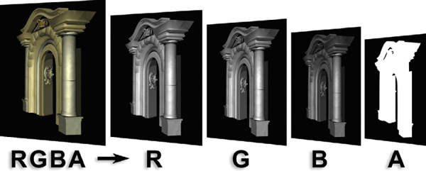
Figure 2-9 A four-channel RGBA image
The RGB channels of a four-channel image contain the picture’s color information, but the matte in the alpha channel is used for compositing. We will soon learn more about using this all-important matte in the next chapter, Compositing CGI.
2.2 ATTRIBUTES OF DIGITAL IMAGES
Now that the structure of digital images is behind us, we can take a look at the various attributes of digital images. They come in different sizes, shapes, and data precision, plus there are differences in how the image data is represented internally. In this section we will start by digitizing an image to see what that is about, then have a ripping good discussion of the difference between image aspect ratio, pixel aspect ratio, and display aspect ratio, three very confusable concepts which we will attempt to de-confuse.
2.2.1 Digitizing Images
Simply put, computers are merely incredibly fast number-crunchers. Even though they perform an enormous variety of functions, in the end all they can do is manipulate numbers (plus a little Boolean logic along the way). As a result, anything they work on must first be reduced to numbers. The letters of the alphabet are even assigned numbers in order to produce a text file such as an email, text message, word processor document, or a book. Sound is converted to numbers to make the MP3 files heard on iPods and CDs. And, of course, pictures must be converted to numbers before the computer can work with them. If it is not first converted to numbers the computer simply cannot deal with it.
Converting a picture (or a sound track) to numbers, or digits, is referred to as digitizing it. Once the computer has the digitized image, everything becomes possible. There are two things to understand about digitizing images. The first is how it is done, and the second is what problems it introduces. We have an example here that will illustrate both points by severely abusing a digitized image. It’s not a pretty picture.

Figure 2-10 Original picture
Figure 2-11 Sampling points
Figure 2-12 Digitized picture
Figure 2-10 starts with the original picture to be digitized. Whenever the image is digitized its colors are measured or “sampled” at regular intervals, represented by the black dots in Figure 2-11. The colors under these sampling points are converted to a number, and then the entire pixel gets that number and becomes a solid color as shown in Figure 2-12. You can actually trace the sampling points becoming pixels by looking, for example, at the sample point on the white collar in the middle of Figure 2-11 and finding the big white pixel in the middle of Figure 2-12. You can similarly map other sample points from various locations around the picture.
The hideous results in Figure 2-12 are caused by the fact that we have sampled the picture by far too few pixels to make a good digitized image, but it neatly illustrates our two key points. First, when an image is digitized it is converted into an array of discrete pixels, each assigned a unique color that was sampled from the original image. Second, when an image is digitized, information is permanently lost. If we had sampled the original picture by, say, 1000 pixels across instead of the absurd 10 pixels in Figure 2-12 we would have a very nice looking digitized image, visually indistinguishable from the original. It would still have some lost information, but the loss would be below the threshold of visibility. The lesson is, the higher the sampling rate the less the loss. We will soon see what kind of problems this loss of information can cause.
2.2.2 Image Resolution
Image resolution refers to how many pixels wide and how many pixels tall a digital image is. For example, if an image were 400 pixels wide and 300 pixels tall the image resolution would be 400 by 300, or written as 400 × 300. An NTSC video image has a resolution of 720 × 486. A standard academy aperture feature film frame has an image resolution of 1828 × 1332. The images from a digital camera might have an image resolution of 3072 × 2048 or more.
Notice that nothing was said about the “size” of the image. This is because the actual display size of an image varies depending on the display device it is viewed on. An obvious example would be a small 11-inch TV screen and a large 32-inch TV screen. The display size is very different, but the NTSC image resolution is identical—720 × 486. A feature film could be projected on a small screen in a little theater or a huge screen in a large auditorium. Again, the display size is very different but the 35mm film image resolution is the same.
We do have to be careful here because the term “resolution” has a very different meaning in other disciplines. The usual meaning for the word outside of digital compositing is not how many pixels in the entire image, but how many pixels per unit of display—that is, how many pixels per inch or dots per centimeter. Where life gets real confusing is when a compositor with his definition of image resolution gets into a conversation with an Adobe Photoshop artist that has the other definition of resolution. To deal with this too-common conundrum there is a special “reluctant” section at the end of this chapter titled DPI designed specifically to sort this out.
2.2.3 Image Aspect Ratio
The aspect ratio of an image is actually a description not of its size or its resolution, but of its shape. It describes whether the image is tall and thin or low and wide. Every job you work on will have an established aspect ratio as well as an image resolution and all of your work must conform to it. The aspect ratio of an image is also frequently needed when trying to fit one image over another. The aspect ratio is simply the ratio of the image’s width to its height, so it is calculated by dividing the image’s width by its height. For example, if the image resolution is 400 × 300, divide 400 by 300 to get an aspect ratio of 1.33, the classic video resolution. Keep in mind that the image aspect ratio applies to the image file itself, not necessarily how it will look when finally displayed. As we will see shortly, sometimes the image aspect ratio and its display aspect ratio differ.
An aspect ratio of 1.0 would mean that the width and height are identical, making it a square image. An aspect ratio of less than 1.0 would be a tall and thin image, and greater than 1.0 the image gets wider as the number goes up. Figure 2-13 illustrates several common aspect ratios starting with a square example of 1.0 followed by the typical NTSC aspect ratio of 1.33, then a couple of common feature film aspect ratios. The key observation to note here is that as the aspect ratio number gets larger the image gets wider.
(To view a high resolution version see www.compositingVFX.com/CH02/Figure 2-13.tif)
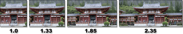
Figure 2-13 The image gets wider as the aspect ratio gets larger
There is one last thing to discuss before we leave the exciting subject of aspect ratios. As we have seen, different disciplines have different ways of describing the same thing. Film folks like to do the math and describe their movie aspect ratios as a decimal number like 1.85 and 2.35. Video people don’t.
Video folks prefer to leave their aspect ratios in the form of ratios like 4 × 3 (4 by 3) and 16 × 9 (16 by 9). They may also write these as 4:3 and 16:9 just to mix things up a bit. If you do the math, a 4 × 3 aspect ratio calculates out to 1.33 (4 ÷ 3) and the 16 × 9 is the same as 1.78 (16 ÷ 9). Again, these are simply two different ways of describing the same shaped image. Having two different ways of doing it, depending on who you are talking to, just adds to the fun of digital compositing.
2.2.4 Pixel Aspect Ratio
As we saw earlier, digital images are made up from pixels. Yes, like images, pixels also have a shape, and that shape is also defined by its aspect ratio. But not all pixels are equal—this is to say, square. A square pixel, like a square image, would have a pixel aspect ratio of 1.0, but many display systems do not have square pixels. Figure 2-14 illustrates the most common non-square pixel aspect ratios you will encounter in production.
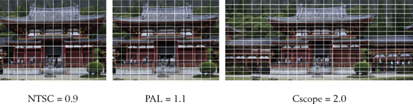
Figure 2-14 Common pixel aspect ratios
The left example illustrates an NTSC video pixel that has a pixel aspect ratio of 0.9, making it tall and thin. The middle illustration depicts a PAL video pixel that has a pixel aspect ratio of 1.1, making it short and wide. While most feature film formats have square pixels, the Cinemascope format (Cscope) is a special wide screen format that has a pixel aspect ratio of 2.0, making its pixels very, very wide. Fortunately, all HDTV (High Definition Television) video formats have square pixels.
These non-square pixels have no impact when they are in their native display environments—NTSC pixels on NTSC television sets, etc. Where they do affect digital compositing is when they are taken out of their native environments, like to a workstation for digital compositing or Adobe Photoshop painting. Suddenly the pixel aspect ratio becomes a major issue that must be dealt with correctly, or there will be trouble. Coping strategies on how to deal with these non-square pixels are addressed in their respective chapters on “Working with Video” and “Working with Film.” At this point we are just trying to get familiar with the troubling concept of non-square pixels in order to set things up for the next section—the display aspect ratio.
2.2.5 Display Aspect Ratio
We have seen how the image aspect ratio describes the shape of the image and the pixel aspect ratio the shape of the pixel. These two factors combine to define the display aspect ratio—the shape of the image after it is projected with its display device. This is altogether important because the aspect ratio of the image may be different than the aspect ratio of the display that it is displayed on, and that difference is caused by the pixel aspect ratio. Not to worry, any compositing program worth its pixels has image viewer options to compensate for non-square pixels so that you can view the image with its proper display aspect ratio. The good news is that if the pixels are square (an aspect ratio of 1.0) then the image aspect ratio and the display aspect ratio are identical. We will see why momentarily.
The display aspect ratio is simply the image aspect ratio multiplied by its pixel aspect ratio. A few examples will serve to make this clearer. We will start with the most severe case, and that is the Cscope film format with a pixel aspect ratio of 2.0 (see Figure 2-14). If a Cscope frame were displayed on your workstation uncorrected, it would look squeezed like the example in Figure 2-15. The image resolution of a Cscope image is 1828 × 1556, so its image aspect ratio would be 1.175 (1828 ÷ 1556). It would appear like this on your workstation monitor because the monitor has square pixels. But the film projector doubles the image in width giving the projected film a pixel aspect ratio of 2.0. If we multiply the pixel aspect ratio (2.0) by the image aspect ratio (1.175) we will get the display aspect ratio of 2.35 (1.174 × 2.0).
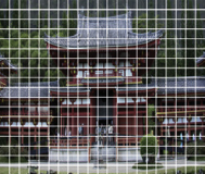
Figure 2-15 Squeezed Cscope image
We know that NTSC and PAL television have an aspect ratio of 1.33, but consider the NTSC image in Figure 2-16. Its resolution is 720 × 486, making its image aspect ratio 1.48 (720 ÷ 486). What is wrong here? We have not factored in the NTSC pixel aspect ratio of 0.9. If we multiply the image aspect ratio of 1.48 by the pixel aspect ratio of 0.9 we will get a display aspect ratio of 1.33 (1.48 × 0.9). If this NTSC image is displayed uncorrected on a workstation it will stretch about 10% in width compared with how it will look on TV because the workstation has square pixels.
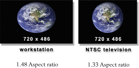
Figure 2-16 NTSC image display aspect ratios
For PAL, the image resolution is 720 × 576 so its image aspect ratio is 1.25 (720 ÷ 576) as shown in Figure 2-17. Here again we don’t get the expected 1.33 aspect ratio for television. When we factor in PAL’s pixel aspect ratio of 1.1 by multiplying it by the image aspect ratio we do get the expected 1.33 (1.25 × 1.1). By the by, if you were to dig out a calculator and check the math here you would find slight discrepancies in the calculated image aspect ratio. This is due to small round-off errors in the numbers used in these examples in order to simplify our story and the math, so it is harmless. If a PAL image is displayed uncorrected on a workstation monitor it will stretch about 10% vertically compared with a television monitor, due to the workstation’s square pixels.
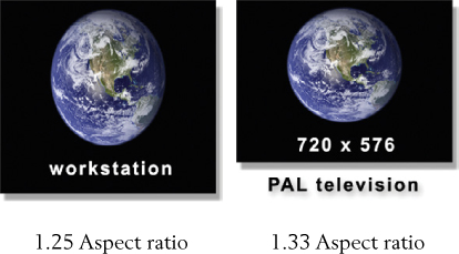
Figure 2-17 PAL image display aspect ratios
(To view high resolution versions see www.compositingVFX.com/CH02/Figure 2-17 ntsc.tif and Figure 2-17 pal.tif)
This brings us to HDTV, which mercifully has square pixels. I like to think this is due in no small part to the vitriolic cries of outraged digital compositors complaining about working with the non-square pixels of NTSC and PAL. Because square pixels have an aspect ratio of 1.0, when the display aspect ratio is calculated by multiplying the image aspect ratio by 1.0 there is no change. The conclusion is that the display aspect ratio and image aspect ratio are the same for images with square pixels.
You have undoubtedly heard that computers only work with ones and zeros. This is literally true. Each one and zero is called a bit (binary digit—get it?), and these bits are organized into 8-bit blocks called bytes. Here is a byte—00000001. Here is another one—11001010. If you group 8 bits into a byte the number of possible combinations of ones and zeros is only and exactly 256, and their values range from 0 to 255. In other words, an 8-bit byte can hold any integer number between 0 and 255. The number of bits being used is what is meant by the term bit depth. If the number of bits was increased to 10 we could make 1024 different numbers. If they were reduced to 4 we could only make 16 numbers. The greater the bit depth, the more numbers we can make.
To relate this back to digital images, if a pixel’s brightness is described by an 8-bit byte then there can only be 256 brightness values ranging from black (0) to white (255). This seems sensible enough. For an 8-bit three-channel RGB image, then, each channel can have only 256 brightness values ranging from 0 to 255. The maximum possible number of different color combinations becomes 256 × 256 × 256 (for all three channels), or about 16.7 million colors. That may sound like a lot of colors, but read on.
Modern compositing packages also support 16-bit images. When the bit depth is increased from 8 to 16 bits per pixel, we now have a whopping 65,536 possible brightness steps from black to white (0 to 65,535). But note this—the black isn’t any blacker nor the white any whiter. There are simply a lot more tiny brightness steps in the 16-bit image compared with the 8-bit image. In fact, the 16-bit image has 256 brightness steps for each one in the 8-bit image. The maximum number of different colors for a 16-bit RGB image becomes 65,536 to the third power, or a tad over 281 trillion. That will usually do it.
Figure 2-18 Smooth sky gradient
Figure 2-19 Banding sky
Now for the part about why you care about all this. The 8-bit image with its 256 brightness steps is barely adequate to fool the human visual system into seeing smooth continuous colors like the sky gradient in Figure 2-18. If such marginal images are heavily processed during compositing (which often happens), the number of brightness steps becomes depleted. Instead of 256 steps there might remain only, say, 100 or less. A smooth gradient cannot be made with only 100 steps of brightness, so the resulting image erupts with banding like the sky in Figure 2-19. (To view a high resolution version of the banding see www.compositingVFX.com/CH02/Figure 2-19.tif). Increasing the bit depth of images protects them from banding. If you start with far more steps of brightness than you need then you can lose some of them without seeing any problems. Therefore it is common practice in digital compositing to “promote” 8-bit images to 16 bits to avoid banding. Better yet, use 16 bits to create the original image in the first place.
2.2.7 Floating Point
The discussion above about bit depth pertained to integer data. That is to say, the 8-bit data, for example, ranged from 0 to 255, using only whole numbers. There were no decimals like 10.3 or 254.993. However, decimals are a very important alternative way to represent pixel values so they are also supported by compositing programs. The computer can easily convert integer data to floating point and Figure 2-20 illustrates how this is done using 8-bit data as an example.

Figure 2-20 Floating-point representation of 8-bit data*
The floating-point value of zero is set to the 8-bit integer value of zero, and the floating-point value of 1.0 is set to 255, the largest number that 8 bits can make. For 16-bit data 1.0 is set at 65,535. Two important benefits and one problem result from working in float (“float” is salty computer talk for floating point).
The first important benefit is that, unlike integer numbers, you can multiply and divide float numbers, which is constantly done in digital compositing. Case in point: suppose you want to multiply two pixels that are 50% gray. Logic tells you that if you multiply 50% times 50% the answer has to be 25%. However, if you are working in 8-bit integer a 50% gray pixel is 128. If you multiply 128 times 128 you get 16,384, a far cry from 25%. If the same problem is done in float, however, it becomes 0.5 times 0.5, which is 0.25, exactly 25%. The float value of 0.25 can then be converted back to an integer value of 64. Much better.
The second benefit of float is to avoid clipping the pixel values. Suppose you wanted to add two 8-bit pixels together, each with a value of 160. The answer will obviously be 320. But since 255 is the largest number we can make with 8-bit integer data the 320 gets whacked (or, more technically, clipped) to 255 by the computer. Data lost, picture ruined. However, if we are working in float the value of 160 becomes 0.625. If we add 0.625 to 0.625 we get 1.25, a value greater than one. While 1.0 is the brightest pixel value that can be displayed on the monitor, the computer does not clip the 1.25 to 1.0. Instead, it preserves the entire floating-point number. No clipping, picture saved.
The problem float introduces is that it is slower to compute than integer. In fact, that is why integer was used in the first place—because it was faster. However, modern computers have become so fast that the speed penalty for working in float is getting less and less over time.
2.2.8 Multiplying Images
In the floating-point discussion above it was pointed out that by using floating-point data the computer could multiply two pixels together. If follows, then, that two images can be multiplied together. Multiplying two images together may sound a bit daft—sort of like multiplying a bird times a rat to get a bat—but in actuality it is a hugely important and common operation when working with digital images. It is at the very core of the compositing process as well as matte and masking operations, so pausing to take a closer look would be a good idea.
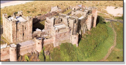
Figure 2-21 Color image

Figure 2-22 Mask
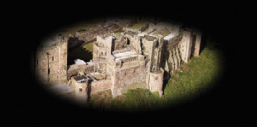
Figure 2-23 Multiplied
Consider the color image in Figure 2-21 and the elliptical mask in Figure 2-22. These two images have been multiplied together and the results are in Figure 2-23. Now let’s follow the action. The white pixels in the center of the mask have a floating-point value of 1.0. When those pixels are multiplied by their partner pixels in the color image the color pixels are unchanged and go to the multiplied image in Figure 2-23 totally in tact. The black pixels around the outside of the gradient have a floating-point value of zero, so when they are multiplied by their partners in the color image the results are zero, resulting in the black region of the multiplied image. The gray pixels around the gradient have a range of values between zero to 1.0, so in that region the multiplied image has pixels that range between black and the original color image, giving it the soft edge fade-off. Multiplying a color image by a mask like this is done all the time in digital compositing.
2.3 IMAGE FILE FORMATS
Every image you receive from or deliver to a client or colleague will be in a file, and files come in a wild variety of different formats. It’s a real zoo out there, and you need to pick your file formats wisely. There are several reasons why you care about this issue. First, if you deliver a file, or one is delivered to you, in a format that the target program cannot read you are dead in the water before you even start. Second, some file formats compress the image file in ways that degrade the image. There are times when this is OK and times when this is not. Third, picking the wrong file format can make the file size much larger than it needs to be. Most folks do not appreciate having their disk space, download time, network bandwidth, and production time wasted.
Before actually looking at the file formats, however, there are a few key concepts to know about certain image types and compression schemes. In this section we will take a look at the difference between photographic images and graphics because the type of image you have mightily affects the choice of compression scheme. The EXR file format gets its own special mention because of its emerging importance in the visual effects industry.
2.3.1 Photographic Images vs. Graphics
There are really two major types of images: photographic images and graphic images. Photographic images are real scenes captured by some kind of camera—digital or film. Their key feature is that their pixel values vary considerably all over the image, thus making them “complex.” Graphics, on the other hand, are basically simple images created with a graphics program or drawn with a paint system such as Adobe Photoshop. Their key feature is that their pixel values don’t vary very much at all over the image.
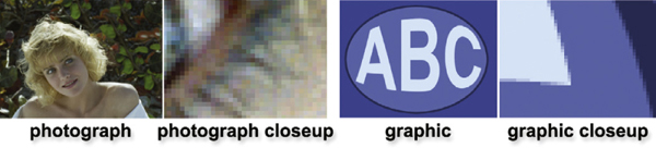
Figure 2-24 Pictures and graphics have very different pixel variations
Figure 2-24 illustrates this profound difference between the two types of images at the pixel level. In the photograph closeup no two pixels are the same color. In the graphic closeup there are large areas of identical pixel values. These differences are used when selecting a compression scheme. A lossless type of compression would be used on the graphic because the file size could be compressed by taking advantage of all the pixels of the same value. Such a scheme would be useless on the photograph and result in virtually no file size reduction. A lossy compression scheme would noticeably damage the graphic, but could go unnoticed in the photograph if not pressed too far.
2.3.2 Indexed Color Images (CLUT)
The file size of any RGB image can be considerably reduced by converting it to an indexed color image. The computer first does a statistical analysis of all the RGB colors in the image, and then produces a Look-Up Table (LUT) of only 256 colors, which represent the closest 256 averages of all the colors in the RGB image. It then creates a one-channel 8-bit “index” image where each pixel is really a pointer or index to one of the colors in the color table. To display the image in color the computer looks at each pixel in the index image, follows that index to its color chip in the LUT, gets that RGB value and displays it on the monitor—like the red arrows in Figure 2-25.
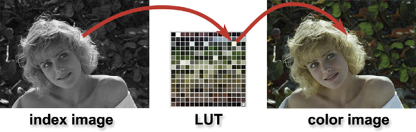
Figure 2-25 An indexed color image
Even though the range of colors is seriously reduced (256 colors instead of 16 million) the resulting color image looks surprisingly good (if you don’t look too closely). The Marcie color image in Figure 2-25 is an actual index color image. The reason it looks so good is that the 256 colors in the LUT are full 24-bit RGB values. Since there are only 256 of them they do not increase the file size by much. A common abbreviation for index color images is CLUT, which stands for Color Look-Up Table.
CLUT images work very well for graphics, especially if the graphic has fewer than 256 colors in it. The CLUT version would then be a lossless compression. Photographic images can be converted to a CLUT, of course, but they get badly hammered in the process. They might look OK for a web site, but not for printing an 8 × 10 portrait.
Almost all file formats offer some kind of data compression feature. Some types of data compression are lossless, meaning that after the compressed file is opened the image is an exact replica of the original. However, some compression schemes are lossy, meaning that the compressed image has suffered some losses, or degradation.
Two predominant lossless compression schemes are RLE and LZW. RLE (Run Length Encoding) is almost always used for rendering CGI images. LZW (Lempel-Ziv-Welch, the guys that invented it) is important because it is available in a great many image file formats. Since these are lossless compression schemes they reduce file size without any degradation of the image. They can also be used together. Use them freely on CGI and graphics knowing that they will not harm your pictures. LZW can be used on photographic images but there will be minimal compression.
Two predominant lossy compress schemes are jpeg and mpeg-2. Jpeg is intended for still images and basically removes fine detail in the image to reduce its file size. It degrades the image quality, and if set too high can degrade it seriously. Mpeg-2 is specifically designed for moving pictures such as video. It starts by performing a jpegtype compression on selected key frames, and then shrinks the in-between frames by constructing a list of what the differences are between the key frames.
2.3.4 EXR
EXR is short for OpenEXR, a floating-point image file format developed by ILM that is fast becoming an industry standard. This makes it very likely that you will encounter it early in your digital compositing career and more likely over time, so it behooves us to take a moment to look at it closely. The next section talks about the various important image file formats, but EXR is both unique and important enough to get its own spot in the sun, especially because it was specifically developed with us compositors in mind. Here is a summary of its main features:

• High dynamic range—designed specifically to accommodate high dynamic range image data such as film scans and photorealistic CGI elements. The dynamic range (darkest to brightest) of an average monitor might be around 150 to one and projected film perhaps 2000 to one, while EXR’s dynamic range is over a billion to one!
• Many channels—while the typical CGI render is a four-channel image, EXR is expandable to any number of channels. The purpose is to avoid having to render the multiple passes of a CGI object into multiple separate files. They can all be in their own channels within one EXR file.
• Lossless compression—designed for feature film work, film frames are large photographic images that take up a lot of disk space and network transfer time. A unique lossless compression scheme is supported that cuts file sizes in half without any degradation to the image and it is very fast to compress and uncompress.
• Short float—a floating-point format, but instead of the usual 32-bit float, implements a unique 16-bit “short float.” This solves the speed penalty usually associated with floating point while maintaining more than enough precision even for feature film work. In other words, the speed of integer with the precision of float.
ILM released OpenEXR to the world as an open standard for free in 2003 in order to rapidly propagate it into the visual effects industry. It has worked. Most 3D animation and compositing programs now support EXR. It has even penetrated the ubiquitous Adobe After Effects and Adobe Photoshop.
2.3.5 File Formats
We cannot discuss every file format in the known universe since that would be an entire book on its own. What we have here is a mercifully brief description of several of the most common file formats that you are likely to encounter in your budding digital compositing career. No effort is made to tell you everything about each file format, as that would be tedious and boring. What is told here is just what pertains to our type of work.
It is standard practice to add an extension to the filename of an image to identify what file format it is. If the file is a tiff format, for example, it would be named “file-name.tif,” a jpeg image would be “filename.jpg,” and so on. Based on this, the file formats are listed below in alphabetical order based on their filename extensions:
• .bmp—a flexible Windows image file format that supports both photographs and graphics. Images can be saved as 8 or 16 bits, BW, RGB, RGBA, and CLUT. No compression.
• .cin—cineon, an older, very specialized file format specifically for 10-bit log film scans. No compression, no options, no nothing. Supports BW, RGB, and RGBA images.
• .dpx—digital picture exchange, a modern file format for 10-bit log film scans that is replacing the cineon format. Supports multiple channels, multiple bit depths, and linear as well as log data. HDTV video frames are sometimes saved in the .dpx format.
• .exr—short for OpenEXR, Industrial Light and Magic’s extended dynamic range file format for working with feature film images. It features floating-point data and the enormous dynamic range of brightness and color required for top-quality feature film work.
• .gif—most commonly seen as an 8-bit CLUT file format for graphics that is extensively used for the web. Includes support for animations in one file and assigns one CLUT color for hard-edged transparency. Also supports 8- and 16-bit images, BW, RGB with lossless compression, but nobody seems to care.
• .jpg—jpeg, or Joint Picture Expert Group, is an older lossy compression file format specifically designed for photographic images. Main feature is the ability to dial in the amount of compression to make the file size smaller, which also effects how much picture information is lost. Excessive compression causes serious loss of picture quality and introduces artifacts.
• .jp2—jpeg 2000, a newer lossy compression file format also specifically designed for photographic images. Based on completely different technology than jpeg, it compresses image files to a smaller size while introducing fewer artifacts.
• .mov—Apple’s® ubiquitous QuickTime® movie file format is used to store moving pictures. The QuickTime file format is actually a “wrapper” that supports a long list of possible compression schemes called codecs (code/decode). While many programs can read QuickTime movies, trouble comes when the movie was compressed with a codec that the program trying to read the file doesn’t have.
• .png—the Windows version of a gif file that supports true transparency.
• .psd—Adobe Photoshop file format that supports separate layers for the various elements of an image. Intended for Photoshop picture editing, so not supported by very many other programs.
• .tga—targa, a Windows-based file format that supports CLUT, BW, RGB, RGBA, 8 bits per channel and lossless compression.
• .tif—tiff, the most important image file format because it is supported by virtually every digital imaging program in the known universe. An extremely flexible and fully featured file format that supports multiple channels, 8- and 16-bit images, and lossless compression. Ideal for CLUT, BW, RGB, RGBA, graphics, photographs, CGI, and virtually every other image type except a compressed photograph (use jpeg or jpeg2000).
• .yuv—a file format specifically for video frames. Many programs can read yuv files and convert them to RGB for display on the monitor, and then write out the results as a yuv file.
2.4 DPI
Even though we shouldn’t have to be doing this in a book on digital compositing, it is unfortunately necessary to digress for a moment to discuss dpi, or “dots per inch,” simply because it is a constant source of confusion and disarray in visual effects. Dpi is a concept used in the print media such as books and magazines. It also shows up in Adobe Photoshop on the Image Size dialogue box as “Resolution.” In the context of printing, resolution means how many pixels are printed per inch of paper. In the context of digital compositing, resolution means the width and height of an image in pixels. Already we are conflicted.
If you had an image that was 100 pixels wide and printed it in a magazine as a one-inch wide picture you would obviously have 100 pixels spread across one inch of paper. The picture would therefore have a print resolution of 100 pixels per inch. For the sake of honoring print tradition, it would actually be referred to as 100 dpi (dots per inch). Now suppose you had a 500 pixel image and printed it as a five-inch picture. The resolution would still be 100 dpi because in one inch of picture you still have 100 pixels. Never mind the fact that the picture is five inches wide. But suppose your 500 pixel image was printed as a one-inch picture. You would now have a 500 dpi image because 500 pixels were spread over one inch. For a given image width in pixels, the smaller it is printed, the more pixels per inch, the greater the dpi. For a fixed picture size, the higher the dpi the sharper the image will be (Figure 2-26).
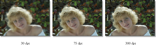
Figure 2-26 Increasing the dpi makes the picture sharper
You can actually watch this in action in Photoshop. Load in any image then go to the Image Size dialogue box. First, uncheck “Resample Image” near the bottom. This tells Photoshop not to change the image “Pixel Dimensions: Width or Height” (what we digital compositors call image resolution). Now go to the “Resolution” window and change the number and watch the “Document Size: Width and Height” values change. Now change the “Width or Height” values and watch the “Resolution” value change. What is happening is that we have locked the image width and height so that the actual pixel counts are not changed while altering the dpi to see how the resulting picture will get printed larger or smaller on paper.
There are two points to this story. The first is that if an image is created in Photoshop for a visual effects shot the question of what the dpi should be may come up. The answer is that the dpi is irrelevant. It is only the image Width and Height in pixels that are important to us. This will confound some Photoshop artists that are print oriented. The second point is that when images are taken from a visual effects shot to Photoshop or to print (such as PR photos) this may also raise the question of the dpi. Again, the dpi is irrelevant; it is the Width and Height in pixels that matters. For print, some may be tempted to scale the image up so it can be printed as a larger picture. If you want the picture printed larger, just lower the dpi.
*Obligatory history lessoon: “pix” is a slang abbreviation of “pictures”, and “el” comes from “element” so pix + element = pixel, meaning “picture element”.
*To the attentive mathematician the floating-point numbers displayed in Figure 2-20 will be seen to be slightly off. For example, the correct calculation of the floating-point value for 128 is 128 ÷ 255 = 0.50196078431. However, the story is easier to follow if things are simply rounded off to the intuitive values used above.