Multilevel Modeling of Longitudinal and Functional Data
McGill University
I signed on to write this commentary because I was confused. Thirty-two years of teaching multivariate statistics to psychology graduate students, and of being a consultant on research projects in a range of disciplines, had not left me with a clear sense of what multilevel analysis was all about. Seemingly related terms in statistics journals, such as hierarchical linear model (HLM), empirical Bayes estimation, random coefficient model, variance component, repeated measures, longitudinal data analysis, latent curve analysis, and even the term multilevel itself seem to have similar but not completely consistent implications. Moreover, my own research preoccupation is with the modeling of functional data, that is, observations that are curves or images, and I wished that I had the links with these areas of statistics better arranged in my mind. So a read through these three fine papers convinced me to organize what I thought I knew, learn some new things, and try to share some of this with readers of this valuable volume. All three papers are solidly data oriented, all three sets of authors were already on my admiration list, and all propose some rather up-market statistical technology for a rather challenging data context. If I can add a little something, either to a reader’s appreciation, or to future research efforts, it will be a great pleasure.
I begin by exploring the term multilevel, which, it appears, means rather different things if applied to data and research designs than it means if applied to models and parameter spaces. Because for me data always have precedence over models and mathematics, I’m happy to agree with the authors in their use of the term. Moreover, more of my focus in what follows will be on data rather than model characteristics, hence, first two multilevel data sections, one on the general situation, and one focused on longitudinal data. There follows two multilevel model sections, again offering a general multilevel framework, followed by specifics for the data of focus. Then we return to consider features of longitudinal data, an important special type of multilevel data. The chapter concludes with a review of some modeling strategies along with an assessment of what these three papers have achieved. The references that have been especially helpful to me are annotated at the end.
To save space, I hope that neither the readers nor the authors will object if I refer to Curran and Hussong; Kenny, Bolger, and Kashy; and Raudenbush as CH, KBK, and R, respectively.
MULTILEVEL DATA
An observation, Yij, is organized on two levels. The lower or most basic level is associated with subscript j = 1, …, ni, and corresponds to the most elementary unit of data that we wish to describe. For CH and R, who consider longitudinal data, this is the value of a variable at the year indexed by j. For KBK, on the other hand, this basic unit is the partner with whom a person interacts. On the other hand, lower level units may, themselves, be collections of variable values. For example, we may refer to an individual’s entire longitudinal record as vector yij, so that the individual is the lower-level unit.
However, observations are also organized by a higher level index i =1, …, m, and this refers to one of m categories within which lower units fall, or within which they are nested. For the National Longitudinal Survey of Youth analyzed by CH, the National Youth Survey analyzed by R, and most longitudinal data, the upper level unit is the individual who is measured at ni time points. The upper level for KBK corresponds to the m = 77 persons, each of whom interacts with a number of partners. The number of lower basic units ni can vary over upper level index i. Upper level units are considered either random or fixed, with random units being categories that will normally change if the data collection process is replicated (e.g., subjects or schools), whereas fixed units are those such as treatment groups that will be reused over replications.
Third and higher-level types of classification of units are often needed, and R, for example, considers schools to be a third level for the Sustaining Effects Data, where students are second- level units, and time points are at the lowest level. This necessitates another subscript, so that the observation in this case would be Yijk.
Covariates are often a part of multilevel data designs, and these may be indicated by the vectors xi and zij, having p and qi elements, respectively, and with the number and nature of subscripts indicating whether these covariates are associated with upper or lower levels of data organization. We shall use xi to refer to covariates for upper-level units and zij for lower-level covariates.
For example, R’s models for the National Youth Survey data use as covariates a constant level, coded by 1, and age, aij (he exchanges the roles of i and j in his notation). This means that the covariate vector zij = (1, aij)t. In fact, as we see, the same covariate vector is used for the upper-level units (individuals), so that a set of covariates may appear twice in the same model, once for modeling lower-level effects and once for modeling upper-level effects. Similarly, CH propose the same multilevel model in their Equations 4.5 to 4.7, with the covariates being, in their notation, 1 and t, (their t corresponding to my j). KBH use the gender and physical attractiveness of the partner as lower-level covariates and subject gender as the upper level covariate.
SPECIAL FEATURES OF LONGITUDINAL DATA
Repeated measures, longitudinal data, and times series are all terms with a long history in statistics referring to measurements taken over time within a sampling unit. Add to these the term functional data, used by Ramsay and Dalzell (1991) to describe data consisting of samples of curves. Each curve or functional datum is defined by a set of discrete observations of a smooth underlying function, where smooth usually means being differentiable a specified number of times. A comparison of Analysis of Longitudinal Data by Diggle et al. (1994) with the more recent Functional Data Analysis by Ramsay and Silverman (1997) highlights the strong emphasis that the latter places on using derivative information in various ways. The more classic repeated measures data are typically very short time series as compared with longitudinal or functional data, and time series data are usually much longer. Most time series analysis is directed at the analysis of a single curve and is based on the further assumptions that the times at which the process is observed are equally spaced and that the covariance structure for the series has the property of stationarity, or time invariance.
The Missing Data or Attrition Problem
Longitudinal or functional data are expensive and difficult to collect if the time scale is months or years and the sampling units are people. Attrition due to moving away, noncompliance, illness, death, and other events can quickly reduce a large initial sample down to comparatively modest proportions. Much more information is often available about early portions of the process, and the amount of data defining correlations between early and late times can be much reduced.
Although there are techniques for plugging holes in data by estimating missing values, a few of which are mentioned by CH and R, these methods implicitly assume that the causes of missing data are not related to the size or location of the missing data. This is clearly not applicable to measurements missing by attrition in longitudinal data. Indeed, the probability of a datum being missing can be often related to the features of the curve; one can imagine that a subject with a rapidly increasing antisocial score in CH’s data over early measurements is more likely to have missing later measurements. I am proposing, therefore, to use the term missing data to refer to data missing for unrelated reasons and the term attrition to indicate data missing because of time- or curve-related factors.
The data analyst is therefore faced with two choices, both problematical to some extent. If only complete data records are used, then the sample size may be too limited to support sophisticated analyses such as multilevel analysis. Moreover, subjects with complete data are, like people who respond to questionnaires, often not typical of the larger population being sampled. Thus, an analysis of complete data, or a balanced design, must reconcile itself, like studies of university undergraduates, with being only suggestive by a sort of extrapolation of what holds in a more diverse sampling context.
Alternatively, one can use methods that use all of the available data. The computational overhead can be much greater for unbalanced designs, and in fact the easily accessible software packages tend to work only with balanced data. In any case, as already noted, results for later times will tend to both have larger sampling variance, due to lack of data, and be biased if attrition processes are related to curve characteristics. Thus, although using “missing-at-random” hole-filling algorithms, such as developed by Jennrich and Schluchter (1986) and Little and Rubin (1987), may make the design balanced in terms of the requirements of software tools in packages such as SAS and BMDP, the results of these analyses may have substantial biases, especially regarding later portions of the curves, and this practice is risky. I must say that my own tendency would be, lacking appropriate full data analysis facilities, to opt to live with the bias problems of the complete data subsample rather than those that attrition and data substitution are all too likely to bring.
Registration Problem
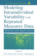
Figure 4.1 displays curves showing the acceleration in growth for ten boys, and we see there that there are two types of variation happening. Phase variation occurs when a curve feature, such as the pubertal growth spurt, occurs at different times for different individuals, whereas the more familiar amplitude variation occurs when two units show differences in the characteristics of a feature even though their timings may be similar. We can see that averaging these curves results in a mean curve that does not resemble any of the actual curves; this is because the presence of substantial phase variation causes the average to be smoother than actual curves.
In effect, phase variation arises because there are two systems of time involved here. Aside from clock time, there is, for each child or subject, a biological, maturational or system time. In clock time, different children hit puberty at different times, but, in system time, puberty is an event that defines a distinct point in every child’s growth process, and two children entering puberty can reasonably be considered at equivalent or identical system times, even though their clock ages may be rather different.
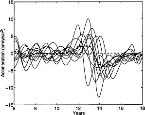
Figure 4.1: Acceleration curves for the growth of 10 boys showing a mixture of phase and amplitude variation. The heavy dashed line is the mean curve, and it is a poor summary of curve shapes.
From this perspective, we can imagine a possibly nonlinear transformation of clock time t for subject i, which we can denote as hi(t), such that, if two children arrive at puberty at ages t1 and t2, then h1 (t1) = h2 (t2). These transformations must, of course, be strictly increasing. They can be referred to as time warping functions. If we can estimate for each growth curve a suitable warping function h such that salient curve features or event are coincident with respect to warped time, then we say that the curves have been registered. In effect, phase variation has been removed from the registered curves, and what remains is purely amplitude variation. The first panel of Figure 4.2 displays the warping functions hi(t) that register the 10 acceleration curves in Figure 4.1. The second panel of Figure 4.2 shows the registered acceleration curves in Figure 4.1.
The multileveling modeling methods considered by these three authors, and in most applications, concern themselves solely with amplitude variation. However, it seems clear that children evolve in almost any measurable respect at different rates and at rates that vary from time to time within individuals. The potential for registration methods to clarify and enhance multilevel analyses seems important. Recent references on curve registration are Ramsay and Li (1998) and Ramsay and Dalzell (1995).
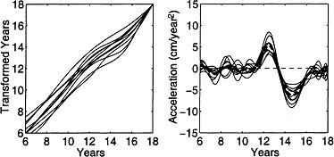
Figure 4.2: The left panel contains the warping functions for registering the growth acceleration curves in Figure 5.1, and the right panel contains the registered curves.
Serial Correlation Problem
Successive longitudinal observations usually display some amount of correlation, even after model effects are removed. Typically, this correlation between successive residuals decays fairly rapidly as the time values become more widely separated. This serial correlation is obvious in CH’s Table 3.1, for example, and we know from studies of human growth that heights measured 6 months apart have correlations between residuals of about minus 0.4. This may be due to “catch-up” processes that ensure that slow growth is followed by more intense growth episodes. Negative serial correlation causes actual observations to tend to oscillate rapidly around a smooth curve that captures the longer-scale effects, whereas positive serial correlation results in slow smooth oscillations. Modeling these serial effects requires introducing some structure in the covariances among successive errors eij. Diggle et al. (1994) have an excellent discussion of these effects, as well as modeling strategies, and all three papers mention the problem. We return to this issue in the modeling sections.
Resolution of Longitudinal Data
The amount of information about a curve that is available in a set of ni measurements is not well captured by ni itself. Let us consider other ways of thinking about this.
An event in a curve is a feature or characteristic that is defined by one or more measurable characteristics.
1. Levels are heights of curves and are defined by a minimum of one observation. The antisocial score of a child at time 1 in CH’s data is a level.
2. Slopes are rates of change and require at least two observations to define. Both CH and R are concerned with slope estimation.
3. Bumps are features having (a) the amplitude of a maximum or minimum, (b) the width of the bump, and (c) its location; they therefore are three-parameter features.
We may define the resolution of a curve as the smallest size on the time scale of the features that we wish to consider.
Discrete observations are usually subject to a certain amount of noise or error variation. Although three error-free observations are sufficient, if spaced appropriately, to define a bump, even the small error level present in height measurements, which have a signal-to-noise ratio of about 150, means that five observations are required to accurately assess a bump, corresponding to twice- yearly measurements of height. More noise than this would require seven measurements, and the error levels typical in many social science variables will imply the need for even more. This is why R says that slope inferences cannot be made with only two observations. We may, therefore, define the resolution of the data to be the resolution of the curve that is well-identified by the data. The five observations per individual considered by CH are barely sufficient to define quadratic trend, that is, a bump, and confining inferences to slopes for these data is probably safer, especially given their high attrition level.
However, the data resolution is not always so low, and many data collections methods under development in psychology and other disciplines permit the measurement of subjective states over time scales of hours and days rather than weeks and months. Brown and Moskowitz (1998) offer an interesting example of higher-resolution emotional state data. Equipment for monitoring physiological or physical data are now readily available with time scales of seconds or milliseconds and with impressive signal-to-noise ratios. The optical motion tracking equipment that is used in studies such as Ramsay, Heckman, and Silverman (1997) has sampling rates of up to 1,200 Hz and records positions accurate to within a half a millimeter.
MULTILEVEL MODELS
Notation
Here we use notation that has become fairly standard in statistics texts and journals, such as Diggle et al. (1994) and Searle, Casella, and McCulloch (1992) as well as for multilevel analysis in other sciences. We shall use β and ui to indicate regression coefficient vectors to be applied to covariate vectors xi and zij, respectively, so that
Yij = xiβ + zijui + eij.
This model can be expressed more cleanly in matrix notation, so we will need to use the vector notation y to indicate a vector containing all of the lower-level observations. The length of this vector is N = Π ni. Within this vector, the lower level index j will vary inside the upper index i. At the same time, we need to gather the covariate vectors xi and zij into matrices X and Z, respectively. These two matrices will both have N rows.
Here is what these matrices look like for R’s rather typical longitudinal data model specified in Equations 2.1 and 2.2, which, when these equations are combined, and we exchange the roles of i and j, is
Yij = β00 + β10aij + u0i + u1iaij + rij
First, let matrix Ti have ni rows and 2 columns; and in column 1 place 1’s, and in column 2 place the centered age values aij. Then the matrix X has 2 columns, and contains
![]()
and matrix Z contains 2 m columns and is
Corresponding to matrix Z, we also define vector u as containing, one after another, the individual covariate vectors ui = (u0i, uli)t.
Upper Model Level
The behavior of observations Yij given fixed values of regression coefficients β and ui is determined by the behavior of the residual or error term eij. In the most commonly used multilevel model, this error distribution is defined to be normal with mean 0. In some applications, it is assumed that these errors are independently distributed for different pairs of subscripts, and that they have variance σ2. However, for longitudinal data where the lower level of data is an observation of an outcome variable at a specific time, this may be too simple. In this setting, therefore, we specify the covariances among errors by gathering the errors eij into a large vector e, just as we did for the observations Yij, and declare in the upper level model that e is normally distributed with mean vector 0 and with variance-covariance matrix of R order N. The upper level model may also be expressed as, conditional on β and u,
y ~ N (Xβ + Zu, R)
or, in other words, given fixed known values of β and u, y has a normal distribution with mean Xβ + Zu and variance-covariance matrix R. Thus, the upper level model for statisticians corresponds to the lowest level of the data. Perhaps this indicates that they see themselves as reporting up to mathematicians rather than down to we scientists on the ground.
Lower Model Level
One of the paradigm shifts in statistics has been the gradual acceptance by statisticians of a Bayesian perspective. The process has been fraught with controversy, and there is no lack of statisticians who would not like to be thought of as Bayesians, but the concept that parameters, too, have random distributions has caught on. According to the Bayesian view, we must now specify the random behavior of our regression coefficients β and u.
Our lower model level assumptions are that (i) β and u are independently distributed, (ii) β is normally distributed with mean β0 and variance-covariance matrix B, and (iii) u is normally distributed with mean 0 and variance-covariance matrix D.
These assumptions imply that the observation vector y is unconditionally normally distributed with mean Xβ and variance-covariance matrix
var(y) = XBXt + ZDZt + R
Upper level (in the model sense) parameters β and u are often called effects, lower model level matrices B, D, and R are called variance components, and coefficient vector β0 can be called a hyperparameter.
Variance Components
Notice that R is N by N, and therefore too large to estimate from the data without strong restrictions on its structure. It is often assumed to be diagonal and of the form σ2I. However, special alternative structures may be required for longitudinal data, and we consider these in the next section.
However, D may also be large, and is of order 2m in the models used by CH and R. Because m may be large, special structural assumptions are required to reduce the number of variances and covariances to be estimated from the data. If we can assume that between-subject covariances are 0, then D has a block-diagonal structure, with the same variance-covariance submatrix, denoted here by C, in each diagonal block, that is, D has the structure
This simplifies things considerably because we now only have to estimate q(q + 1)/2 variance components. For CH’s example, q = 2, and C is specified in their Equation 3.1. However, sometimes this independence between upper data level units is not sensible; schools as an upper level, for example, which are geographically close, will share many features in common, and their effects should be considered to be correlated.
Parameter independence assumption i is especially important and is perhaps the central structural characteristic of the multilevel model. It asserts that lower level variation in the data sense is unrelated to higher level variation. There are certainly situations where this might be challenged. For example, we might suppose that where lower level units are students and upper level units are schools, certain types of students will respond differently to being placed in certain types of schools, such as parochial, than they will in other types, such as public schools. In fact the assumption is critical to methods for fitting the model.
Assumptions ii and iii indicate, by their specifications of the mean vectors for β and u, that the general or upper-level mean structure is determined by hyperparameters 0, and that lower-level unit means are centered on this mean structure.
Effects as Fixed or Determined by Further Covariates
A specialization of this model is often assumed; the upper data level parameter is declared to be a fixed parameter, which corresponds to the assumption that B–1 → 0. This case is referred to as the mixed multilevel model. In this case, the variance-covariance matrix for y simplifies to
On the other hand, because we can think of β as a random variable, we can propose a linear model for its variation. This is what CH do in their Equations 3.8 and 3.9. Consequently, let W be a p by r matrix of covariates for modeling β, and let α be a vector of r regression coefficients for the model β = Wα + e*. Then we have
var(y) = XWBWtXt + ZDZt + R
where B is now the variance-covariance matrix for α. Actually, this does not really require a modification of our multilevel model notation because the net effect is simply to replace X by XW, and β by α, and this is therefore formally the same model.
Multilevel Modeling Objectives
The multilevel model does three things. First, it specifies a relatively specific covariance structure for observation vector y. The smaller the numbers of columns for X and Z, and/or the more specialized their structure, the more restrictive this model is. The papers of CH and R offer examples of how a simple initial covariance structure specification can be incrementally extended, with a test after each extension indicating whether the fit to the observed variance covariance matrix has significantly improved. Moreover, as we shall see in discussing longitudinal data, there is the potential in most multilevel software to further specialize the structure of the two variance-covariance matrices D and R.
Secondly the multilevel model is especially powerful for estimating lower-level data effects defined by the ui′s. It is often the case that there are few measurements within upper-level units to define these effects, or in extreme cases insufficient data to define them uniquely, but the model permits each unit to borrow information from other units to supplement sparse or missing information. The result is much like increasing the sample size for each unit. This borrowing of strength depends, first, on the data within a unit being relatively weak, either because of the limited number of observations available or because of the high noise level in measurements, and second on the degree of uniformity of variation across upper level units that is, the extent to which variance component matrix D is small relative to error component R.
Finally, upper model level effects captured in β are often the main interest and in this multilevel analysis shares goals with ordinary multiple regression. Indeed, β may be captured by averaging across equivalent lower level effects within the ui′s. This is what KBK aim at in their use of ordinary and weighted least squares methods, and they are quite right to point out that, relative to this task, there may be little achieved by going to the more demanding multilevel technology. How important is it to get the variance-covariance structure right, if all we need are upper-level fixed effect estimates? Diggle et al. (1994) suggest that in many situations a simple variance components model, such as that in classical repeated measures ANOVA, may be preferable from the perspective of effect estimation, even when the data confirm a more complex model. I tend to agree; when the sample size is modest, it’s more important to conserve degrees of freedom for error by economizing on the model than pulling out all the stops to make bias small.
However, in social science applications, one has the impression that the primary focus is on estimating variance components, so that the multilevel model belongs squarely in the long tradition of such models, which includes principal components, factor, and canonical correlation analysis as well as structural equation modeling. Both CH and R model how well the fit to the data improves when both effects and variance components are added to an existing model.
SPECIAL FEATURES OF LONGITUDINAL MODELS AND FUNCTIONAL DATA
Let us now have a look at modeling longitudinal data, with the possibility that the number of observations ni may be rather larger than for the data sets considered by CH and R. These remarks are selected from material in Ramsay and Silverman (1997).
Within-Subject or Curve Modeling
There are two general approaches to modeling curves f:
1. Parametric: A family of nonlinear curves defined by a specific model is chosen. For example, test theorists are fond of the three-parameter logistic model, P(θ) = c + (1 – c)/{1 + exp[–a(θ – b)]}, for modeling the relationship between the probability of getting a test item correct as a function of ability level.
2. Nonparametric: A set of K standard fixed functions ϕk, called basis functions, are chosen, and the curve is expressed in the form
f(t) = α1θ1(t) + α2θ2(t) + … + αkθk(t)
The parametric approach is fine if one has a good reason for proposing a curve model of a specific form, but this classic approach obviously lacks the flexibility that is often called for when good data are available.
The so-called nonparametric approach can be much more flexible given the right choice of basis functions and a sufficient number of them, although it is, of course, also parametric in the sense that the coefficients k must be estimated from the data. However, the specific functional form of the basis functions tends not to change from one application to another. However, this approach is linear in the parameters and therefore perfect for multilevel analysis. Here are some common choices of basis functions:
1. Polynomials: θk(t) = tk–1. These well-known basis functions (or equivalent bases such as centered monomials, orthogonal polynomials, and so on) are great for curves with only one or two events, as defined previously. A quadratic function, for example, with K = 3, is fine for modeling a one-bump curve with 3 to 7 or more data points. These bases are not much good for describing more complex curves, though, and have been more or less superseded by the B-spline basis described subsequently.
2. Polygons: θk = 1 if j = k, and 0 otherwise. For this simple basis, coefficient αk is simply the height of the curve at time tk, and there is a basis function for each time at which a measurement is taken. Thus, there is no data compression; and there are as many parameters to estimate as observations.
3. B-splines: This is now considered the basis of choice for nonperiodic data with sufficient resolution to define several events. A B-spline consists of polynomials of a specified degree joined together at junction points called knots, and is required to join smoothly in the sense that a specified set of derivatives are required to match. The B-spline basis from which these curves are constructed has the great advantage of being local, that is, nonzero only over a small number of adjacent intervals. This brings important advantages at both the modeling and computational levels.
4. Fourier series: No list of bases can omit these classics. However, they are more appropriate for periodic data, where the period is known, than for unconstrained curves of the kind considered by CH and R. They are, too, in a sense, local, but in the frequency domain rather in the time domain.
5. Wavelets: These basis functions, which are the subject of a great deal of research in statistics, engineering and pure mathematics, are local simultaneously in both the time and frequency domain and are especially valuable if the curves have sharp local features at unpredictable points in time.
Which basis system to choose depends on (a) whether the process is periodic or not and (b) how many events or features the curve is assumed to have that are resolvable by the data at hand. The trick is to keep the total number K of basis functions as small as possible while still being able to fit events of interest.
Basis functions can be chosen so that they separate into two orthogonal groups, one group measuring the low-frequency or smooth part of the curve and the other part measuring the high-frequency and presumably more variable component of within-curve variation. This opens up the possibility of a within-curve separation of levels of model. The large literature on smoothing splines follows this direction, and essentially uses multilevel analysis, but refers to this as using regularization.
Variance Components
We have here the three variance components: (a) R containing the within-curve variances and covariances, (b) D containing the second level variances and covariances, and (c) B containing the variances and covariances among the whole-sample parameters α.
The behavioral science applications that I’ve encountered tend to regard components in R as of little direct interest. For nonlongitudinal data, it is usual to use R = σ2I, and, as Diggle et al. (1994) suggest, this may even be a wise choice for longitudinal data because least squares estimation is known to be insensitive to mis-specification of the data’s variance-covariance structure. However, in any case, the counsel tends to be to keep this part of the model as simple as possible, perhaps using a single first-order auto-correlation model if this seems needed. More elaborate serial correlation models can burn up precious degrees of freedom very quickly and are poorly specified unless there are large numbers of observations per curve.
It is the structure of D that is often the focus of modeling strategies. If, as is usual, between-subject covariances are assumed to be 0, then we noted previously that D is block-diagonal and the m submatrices C in the diagonal will be of order K and all equal. Both CH and R consider saturated models in which the entire diagonal submatrix is estimated from the data. Of course, as the number of basis functions K increases, the number of variances and covariances, namely K(K + 1)/2, increases rapidly. The great virtue of local basis systems, such as B-splines, Fourier series, and wavelets, is that all covariances sufficiently far away from the diagonal of this submatrix can be taken as 0, so that the submatrix is band-structured. The PROC MIXED program in the SAS (1995) enables a number of specialized variance-covariance structures.
The contents of B will be of interest only if the group parameters in β are considered random. This seems not often to be the case for behavioral science applications.
CONCLUSIONS
Multilevel analysis requires a substantial investment in statistical technology. Programs such as SAS PROC MIXED can be difficult to use because of unfriendly documentation, poor software design, and options not well adapted to the structure of the data at hand. Although this is not the place to comment on algorithms used to fit multilevel models, these are far from being bulletproof, and failures to converge, extremely long computation times, and even solutions that are in some respect absurd are real hazards. Indeed, the same may be said for most variance components estimation problems, and there is a large and venerable literature on computational strategies in this field. The best known variance components model for behavioral scientists is probably factor analysis, where computational problems and the sample sizes required for stable estimates of unique variances have led most users with moderate sample sizes to opt for the simpler and more reliable principal components analysis.
The emphasis that CH and R place on testing the fit of the various extensions of their basic models might persuade one that fitting the data better is always a good thing. It is, of course, if what is added to the model to improve the fit is of scientific or practical interest. In the case of multilevel models, what are added are the random components and whatever parameters are used to define the variance-covariance structures in D and R.
On the other hand, adding fitting elements may not be wise if the effects of interest can be reasonably well estimated with simpler methods and fewer parameters. For example, if there is little variability in the curve shapes across individuals, then adding random coefficients burns up precious degrees of freedom for error. The resulting instability of fixed effect parameter estimates, and loss of power in hypothesis tests for these effects, will more than offset the modest decrease in bias achieved relative to that for a simple fixed effects model. As for variance components, is worth saying again along with Diggle et al. (1994) and others that modeling the covariance structure in D and R will usually not result in any big improvement in the estimation and testing of the fixed effect vector β. KBK have added an important message of caution in this regard.
If you are specifically interested in the structure of D and/or R, and have the sample size to support the investigation, then multilevel analysis is definitely for you. If you want to augment sparse or noisy data for a single individual by borrowing information from other individuals, so that you can make better predictions for that person, then this technique has much to offer. However, if it is the fixed effects in β that are your focus, then I wish we knew more about when multilevel analysis really pays off. If you have longitudinal data, it might be worth giving some consideration to the new analyses such as curve registration and differential models emerging in functional data analysis. To sum up, which method to use very much depends on your objectives.
REFERENCES
Brown, K. W., & Moskowitz, D. S. (1998). Dynamic stability of behavior: The rhythms of our interpersonal lives. Journal of Personality, 66, 105–134.
Diggle, P. J., Liang, K.-Y., & Zeger, S. L. (1994). Analysis of longitudinal data. Oxford: Clarendon Press.
Jennrich, R., & Schluchter, M. (1986). Unbalanced repeated-measures model with structured covariance matrices. Biometrics, 42, 809–820.
Little, R. J. A., & Rubin, D. B. (1987). Statistical analysis with missing data. New York: John Wiley and Sons.
Ramsay, J. 0., & Dalzell, C. (1991). Some tools for functional data analysis (with discussion). Journal of the Royal Statistical Society, Series B, 53, 539–572.
Ramsay, J. O., & Dalzell, C. (1995). Incorporating parametric effects into functional principal components analysis. Journal of the Royal Statistical Society, Series B, 57, 673–689.
Ramsay, J. O., Heckman, N., & Silverman, B. (1997). Spline smoothing with model-based penalties. Behavior Research Methods, 29(1), 99–106.
Ramsay, J. O., & Li, X. (1998). Curve registration. Journal of the Royal Statistical Society, Series B, 60, 351–363.
Ramsay, J. O., & Silverman, B. W. (1997). Functional data analysis. New York: Springer.
SAS Institute. (1995). Introduction to the MIXED procedure course notes (Tech. Rep.). Cary, NC: SAS Institute Inc.
Searle, S. R., Casella, G., & McCulloch, C. E. (1992). Variance components. New York: Wiley.