
17
Spatial Data Acquisition and Processing
The topic of spatial signal processing is now approached to draw attention to the fact that the anti-aliasing signal processing technology described in this book was initially developed for handling signals in the time and frequency domains but is also applicable in the area of spatial signal processing vital for all types of radar systems. While various types of problems could be attacked on the basis of this technology, the following discussions are focused on the issue of the complexity reduction of large-aperture antenna arrays. Specifically, the potential of pseudo-randomization of large-aperture antenna arrays is considered and evaluated as an approach applicable for reducing the number of sensors in the array. To achieve good results in this area, it is suggested that the positive experience obtained at signal processing in the time domain can be adjusted to the specifics of spatial signal processing. The rationale of this approach is based on the fact that irregular taking of signal sample values in the time domain is equivalent to the irregular spacing of sensors in the array.
Although historically the problems of randomizing the temporal signal processing have received much more attention than the analogous problems of spatial data acquisition and processing, the potential usefulness of deliberate randomization in this area has not been overlooked. A number of publications provide evidence of this. However, at first glance, these publications have nothing to do with randomized processing of signals. They are mainly works dealing with radar antennae. The fact that a number of radar characteristics can be enhanced by randomizing their antenna designs had already been discovered in the early 1960s. It was found that when antenna sensor elements are spaced randomly rather than regularly, undesirable aliasing effects are reduced and other improvements in system functioning can be achieved.
A survey of the research results obtained in the field of array signal processing, the theory of which is relatively well developed, lies beyond the scope of this book. To establish the methodological, terminological and notation basis for the following discussions, a brief description of the principles and relationships relevant to the antenna arrays and array signal processing is given in Section 17.1. Typical spatial signal processing subsystems, usually included in the structures of these array systems, are considered.
Although antenna arrays are used for signal transmission or receiving, the central problem in array signal processing is beamforming. Proper beamforming is essential for concentrating signal energy in a required direction at their transmission and also allows an estimation to be made of the direction of signal arrival at their receiving. While transmission and receiving of signals seem to be distinctly different operations, the beamforming procedures in both cases have much in common. This allows just one of these cases to be considered and to extend the results of the analysis over both areas. Following this reasoning, the signal receiving case is selected as the basis for studies of the suggested specific beamforming techniques suitable for complexity reduction of the array signal processing systems. The discussions concern, first of all, various aspects of the signal direction of arrival (DOA) estimation.
17.1 Sensor Array Model
Consider a linear array of sensors shown in Figure 17.1(a). Suppose that the sensors are distortion-free, isotropic (capable of receiving signals from all directions equally well) and spaced equidistantly. To simplify consideration of the basic principles of such array functioning, suppose also that the signal impinged on the array from a far-field source is described as a narrowband signal with a common centre frequency f or as a nonmodulated sinusoidal carrier at the frequency f. Assume that the angle between the signal plane and the array axis is equal to Θ. In this situation, the signals received by sensors 2, 3, 4,... are delayed with respect to the signal received by sensor 1 and these delays depend on Θ and the intervals d, 2d, 3d,... between the respective sensors. Indeed, the signal at sensor 2 is delayed for a time interval τ2 during which the signal covers the distance d sin Θ and as the signal propagation speed is equal to c, then c τ2 = d sin Θ or τ2 = (d/c) sin Θ. For the kth sensor, the delay
![]()
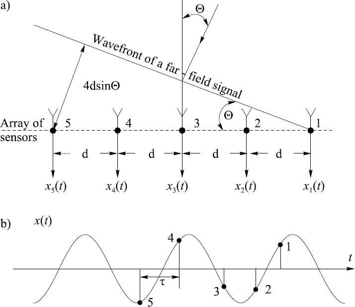
Figure 17.1 Basic array model: (a) delays in signal paths to various sensors depending on the signal arrival angle; (b) array signal formed from digital sample values taken off the sensors at their simultaneous sampling
As the phase shift between the output signals of sensors is ϕ = −2π fτ radians, the phase shift between the adjacent sensor outputs is given as
![]()
Now suppose that all sensor outputs are sampled simultaneously and the respective signal values are read out in this way. Obviously, all these readings are from one and the same sinusoid and intervals between the sample values (Figure 17.1(b)) are equal to the delays mentioned. On the other hand, this sample sequence forms a discrete signal depending on the signal source frequency and location. This array signal
![]()
where A is the amplitude of the received signal, dk is the coordinate of a sensor (with respect to sensor 1) and Ω and ϕ are the wavenumber (spatial frequency) and the array signal phase respectively. It can be seen from Figure 17.1 that Ω = sin Θ (f/c) and Equation (17.3) can be rewritten as

Now suppose that there are m = 1, 2, 3,..., M rather than one signal sources. In this case the received signals, arriving from various directions, add up so that the resulting sequence of the sensor output signal sample values, taken repeatedly at time instants tn, can be considered as the following vector:
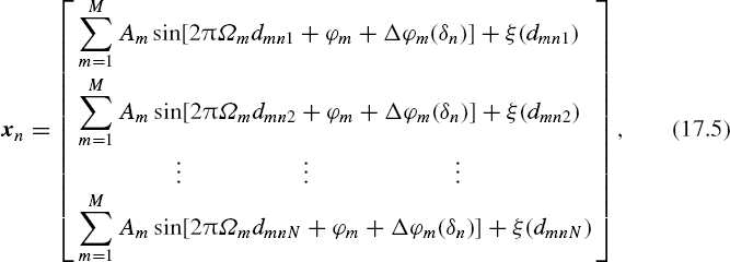
where Am, Ωm and ϕm are amplitudes, wavenumbers and phases of the array signal components respectively, ξ(dmnk) are the noise sample values and Δϕm(δn) are the additional phase delays that appear in special cases when additional delays dn are inserted. Note that when the sensor coordinates are denoted as dmnk, it is presumed that this coordinate may change from one instant tn to another. As that is usually not the case (the sensor positions are fixed), these coordinates can be denoted as dmk.
In more general and specific cases, the signals impinged on an array should be considered as being wideband or narrowband rather than one sine function. Then, naturally, its definition is more complicated.
17.2 Temporal and Spatial Spectra of Array Signals
While the application area of arrays covers a large variety of tasks, solution of every one of them is based, in some way, on relationships of array signal temporal and/or spatial spectra. Basic relationships of this kind will be considered.
Suppose that the far-field signals impinged on a linear array of the type considered above are sufficiently well approximated by a finite number of complex exponential functions. Suppose also that there are altogether m signal sources. Then the signal of the mth source can be written as
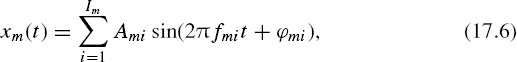
where Ami, fmi and ϕmi are the amplitudes, frequencies and phases of the signal components respectively and Im is the number of components in the signal emitted by the mth source.
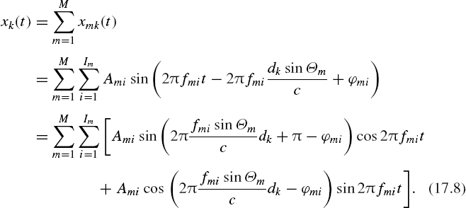
The first sensor will be chosen as a reference point in time and in distance. Then, if the distance to the kth sensor is dk and the arrival angle of the signal from the mth source is denoted by Θm, the component of the kth sensor output signal coming from the mth signal source can be given as

The complete output signal of the kth sensor, containing components coming from all signal sources, can then be defined as
The function A sin(2πft + ϕ) can be represented in the following form:
![]()
where a = A sin ϕ and b = A cos ϕ.
The coefficients a and b are orthogonal projections of the sine function on cos 2πft and sin 2πft. Suppose that a snapshot multitude {xk(tn)}, n = ![]() , has been obtained and that these data have been decomposed by applying some high-performance method and that parameters of the signal components as well as the orthogonal projections have been estimated as a result of temporal spectral analysis with errors not exceeding some given margins. Then two essential cases can be distinguished.
, has been obtained and that these data have been decomposed by applying some high-performance method and that parameters of the signal components as well as the orthogonal projections have been estimated as a result of temporal spectral analysis with errors not exceeding some given margins. Then two essential cases can be distinguished.
17.2.1 When Signal Source Frequencies Do Not Overlap
Suppose that the ith frequency of the mth signal source does not overlap any other frequency of the other signal sources. Then the orthogonal projections corresponding to this frequency, which follows from Equation (17.8), are
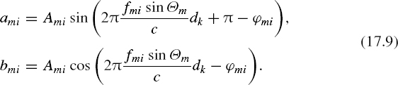
It can be seen from Equations (17.9) that these projections can be interpreted as spatial sinusoidal functions with sample values obtained at points dk. To estimate the wavenumbers Ωmi, spatial spectral analysis of data {ami, bmi} can be performed. According to Equation (17.8),
![]()
It follows from Equation (17.10) that
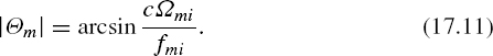
To determine the sign of Θm, Equations (17.9) are rewritten as
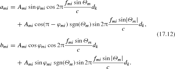
Then the orthogonal projections ami and bmi can be given in the following form:

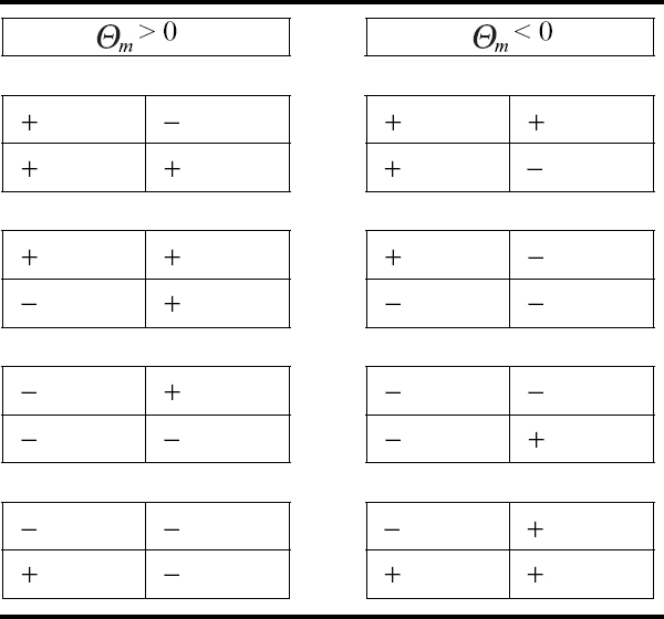
In order to determine the sign of Ωm, Table 17.1 displays the signs of these projections at all possible positions of the phase angleϕmi (it can be in any of the four quadrants). The amplitudes and phases of the respective sine functions can also be determined from the projections given in (17.13).
17.2.2 When Signal Source Frequencies Overlap
Suppose that some of frequencies in spectra of signals coming from different signal sources overlap. Assume that the frequency fmi is common for all signal sources and denote it by f1. Then the projections corresponding to this frequency, obtained in the course of the temporal spectral analysis as follows from Equation (17.8), can be written as
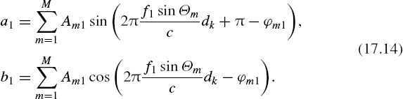
As Θm differs for various signal sources, then projections a1 and b1 can be interpreted as M sums of sine functions at the following wavenumbers:
![]()
Now Equations (17.14) can be rewritten as
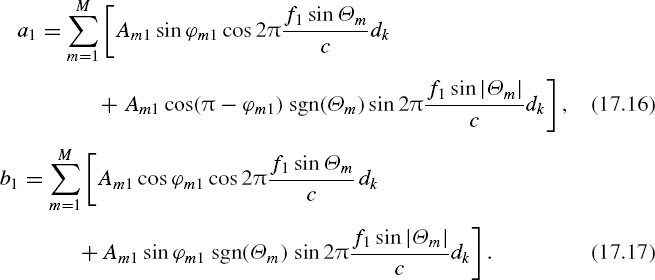
To estimate wavenumbers Ωm, m = ![]() , decomposition of a1 and b1 has to be carried out. As the frequency f1 has been estimated at the stage of the temporal spectral analysis, then, by applying Equation (17.14),
, decomposition of a1 and b1 has to be carried out. As the frequency f1 has been estimated at the stage of the temporal spectral analysis, then, by applying Equation (17.14),
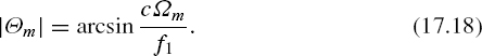
Amplitudes, phases and signs of the arrival angles Θm then can be estimated for all wavenumbers Ωm in the same way as in the case considered above where frequencies do not overlap.
17.2.3 Aliasing in the Spatial Domain
Signal processing as described so far in this section is commonly used for spatial spectrum analysis of a signal received by an array of sensor elements. The temporal signal sampling is then periodic and the sensors in the array are placed equidistantly. Up to certain temporal and spatial frequencies this approach represents a good technical solution to the problem of spatial signal filtering. However, there are limitations. The upper frequency of the signal temporal spectrum is limited, as usual, by the sampling frequency used at the analog-to-digital conversions of the sensor output signals. Obviously this spectrum should not exceed a frequency equal to one-half of the sampling rate.
The minimal wavelength of array signal components is limited by the value d of the interval between the array elements. To guarantee that there is no aliasing, at least two samples from a signal wavelength should be taken, i.e. λmin ≥ 2d and Ωmax = 1/λmin. If the wavenumber of an array signal component exceeds the given limit, aliasing occurs. Clearly, there is a row of indistinguishable wavenumbers that is analogous to the indistinguishable temporal frequencies. As the distance between the array signal digital values is equal to d, the following wavenumbers completely overlap and are accepted by regular arrays as one and the same:
![]()
The aliasing effect is well known and in array beam characteristics it is displayed as the so-called grating lobes. This effect has somehow to be avoided. Otherwise spectra of the signals and noise outside the alias-free range will overlap the spectra within this range and distort the results of signal processing.
The obvious way of enlarging the range free of spatial aliasing is to place sensors closer. However, if this approach is used then, depending on the number of sensors for a given aperture, the complexity of such arrays and of their signal processing systems is directly tied to the required wavenumber range of the spatial spectrum analysis to be performed. There are other problems as well. For instance, cross-interferences between sensors do not allow the sensors to be placed too close, thus limiting the achievable upper boundary of this range.
The fact that the inability to distinguish certain spatial signals is caused by the regularity of their sample value taking procedure was recognized a long time ago and there have been attempts to avoid such aliasing by spacing array elements randomly. However, so far they have not led to sufficiently good results. It seems that the main obstacle preventing the achievement of significant progress in this direction is lack of sufficiently well-developed special digital signal processing techniques that are successful in this area. That is the reason why this topic is included for consideration in this book. There is clearly an analogy between conditions for signal processing in the spatial and the time domains. This means that some part of the suggested advanced signal processing techniques based on nonuniform temporal signal sampling could also be exploited for alias-free processing of array signals. On the other hand, conditions for array signal processing are also quite specific. Therefore it is often not obvious how the positive experience gained in the area of processing nonuniformly sampled temporal signals could be transferred to the area of array signal processing. The discussions in the following sections should help to clarify this matter to some extent.
The potential possibility of array complexity reduction is based on the assumption that if the intervals between sensors in arrays are not equidistant and special anti-aliasing techniques are applied then these intervals between sensors do not necessarily have to be less than half of the shortest wavelength of the array signal components. If that is the case, then the number of sensors in the array with the same aperture and complexity of the array, directly related to the quantity of used sensors, can be reduced. The central issue of this matter, of course, is elimination of aliasing.
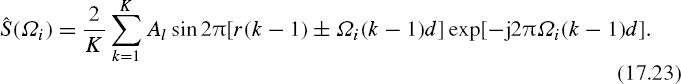
Discussions of this issue will start by considering the spectrum analysis of spatial signals taken off a linear array of isotropic distortion-free sensor elements. Suppose that the obtained array signal reflects a signal impinged on the array that comes from a direction Θ and can be described as an unmodulated sinusoidal carrier. The estimate of the spatial spectrum for a single simultaneous reading of the sensor outputs can be written as
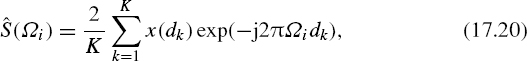
where Ωi is the considered wavenumber and K and dk are the number and the coordinates of the sensors respectively. Suppose that the array signal is a sine function at one of the wavenumbers:
![]()
where Ωs is the array signal spatial sampling rate and is inversely proportional to the distance (mean distance) between the sensors. As the power spectrum does not depend on the signal phase, to simplify the expressions the signal phase can be omitted and Equation (17.20) can be rewritten as

Properties of this estimate depend to a large extent on the positions of the sensors. Consider the case where they are spaced equidistantly with the interval d between them. Then, apparently, dk = (k – 1)d, Ωs = 1/d and estimate (17.22) becomes
This expression clearly shows that when the sensors are spaced equidistantly, the value of the power spectrum estimate at Ωi is the same for all values of r. This means that they are the same for all array signal components at wavenumbers belonging to the row (17.21) if only the amplitudes Al of these components are the same.
The situation is quite different when the intervals between the sensors are not equal. Then the estimate (17.22) will differ at various wavenumbers (at various values of r), which actually means that under these conditions it should be possible to suppress the aliasing effects. This suggests that it should be possible to diminish the negative effect of aliasing by spacing the sensor elements irregularly. Consequently, by applying this technique of array irregularization, it should be possible to use a lesser number of sensors in arrays, because the upper boundary of the required wavenumber range is then no longer determined by the mean distance between the sensors. The computer simulation results given below confirm this presumption.
17.3 Beamforming
Beamforming for arrays is the most important function allowing signal energy to be concentrated in a specific direction or to tune the array in a given direction so that it becomes most sensitive to signals coming from that direction while suppressing all signals and noise received from other directions. Figure 17.2 illustrates the classical direct method for beamforming in the case of signal reception.
When a signal is impinged on a linear array from a direction characterized by the signal arrival angle Θ, as shown in Figure 17.2(a), this signal is received by separate sensors delayed for time intervals τ2, τ3, τ4, τ5 (τ1 = 0). If the delays in the sensor channels are equalized by inserting additional delays, as shown in Figure 17.2(b), and then a reading of the sensor output values is taken simultaneously, the same spatial signal sample value will be obtained at all sensors. Therefore, these outputs can be summed as shown and amplification of the signal, received from the direction to which the array has been tuned by inserting the indicated specific delays, will result while signals coming from other directions will be suppressed.
It can be shown that the signal at the output of the adder is given as
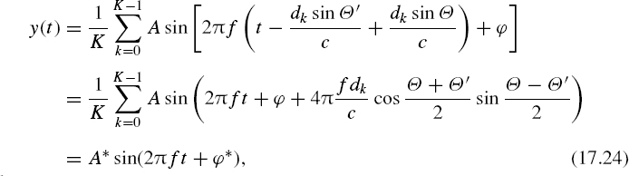
where
![]()
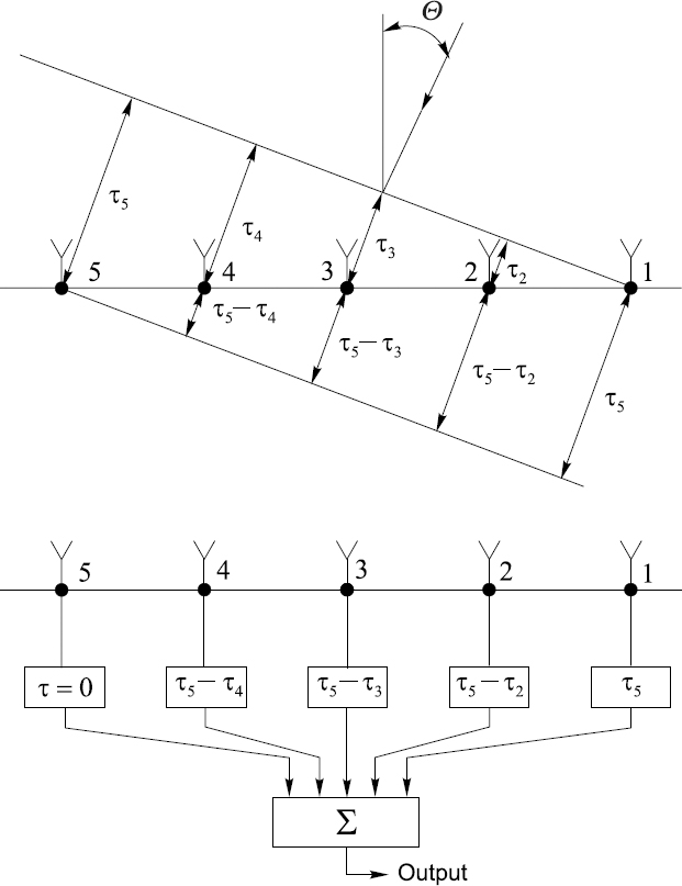
Figure 17.2 Illustration of the direct beamforming principle
and, in turn,
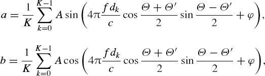
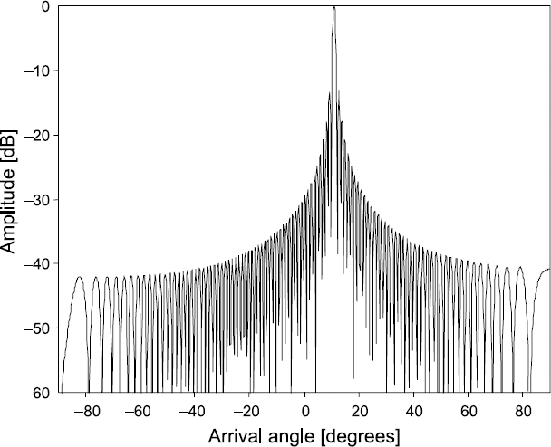
Figure 17.3 Directional pattern of an array of 128 equidistantly spaced sensors (Θ = 11°)
where Θ is the signal arrival angle and Θ′ is the angle to which the array has been tuned. The directional pattern of such an array, containing 128 equidistantly spaced sensors, is shown in Figure 17.3. The array is tuned to Θ = 0°. The directional pattern is obtained on the basis of Equation (17.24) by varying the signal arriving angle. Signals arriving from angles differing from Θ are significantly suppressed.
To see what happens under other conditions the sensor number in the same aperture is reduced to 32. In this case the array directional pattern is as shown in Figure 17.4. It can be seen that aliasing occurs and corresponding grating lobes appear. To avoid aliasing and suppress the grating lobes in this way, the sensors should be spaced in the array irregularly. The obtained directional pattern of such an array is given later in Figure 17.9 and is commented on in Section 17.5.
17.4 Signal Direction of Arrival Estimation
To estimate an array signal direction of arrival (DOA) and the received signal parameters, both temporal and spatial spectral analyses have to be carried out. When this kind of signal processing is considered, it soon becomes clear that there are several possible ways of approaching the task of the DOA.
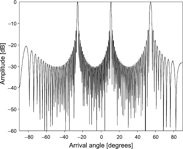
Figure 17.4 Directional pattern of a regular array of 32 sensors under aliasing conditions (Θ = 11°)
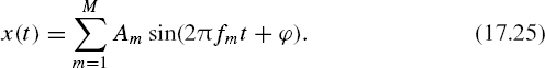
To simplify the following analysis and taking into account the fact that for DOA estimation a single sine function model of signals is applicable, the basic spectral analysis approaches are considered in the case where there are M signal sources and the signal x(t) received by all sensors can be given as
Then the signal sample value xkn taken off the kth sensor at the instant tn is described by the following equation:
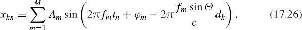
It can be seen that there are two variables: tn and Θ. One of them can be taken as fixed and the other can be varied. Hence there are two possible ways to deal with the analysis of this equation. They are illustrated by Figures 17.5(a) and (b). Both approaches will be considered.
Suppose that time is considered as a variable and Θ is fixed. In other words, the changing time sensor output signals are considered separately for each sensor. This approach corresponds to the scheme given in Figure 17.5(a) and means that the temporal spectral analysis is performed first and the spatial spectral analysis is carried out by processing the sequence of the Fourier coefficients obtained in the first step. Indeed, equation (17.26) can be rewritten as follows:
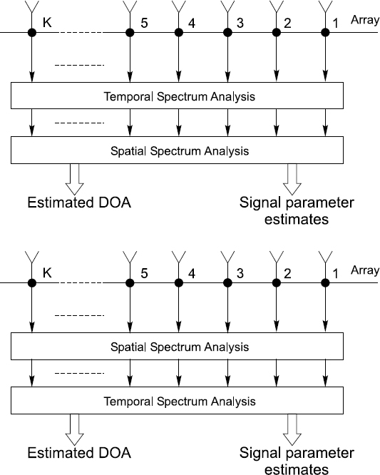
Figure 17.5 Two possible approaches to an estimation of the DOA
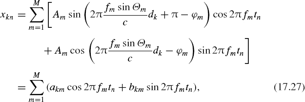
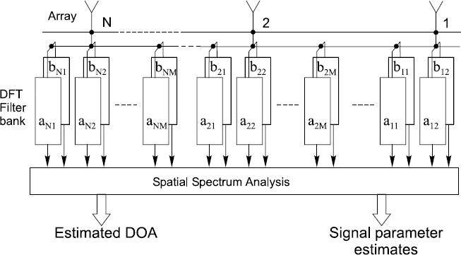
Figure 17.6 Implementation of the DOA estimation scheme on the basis of a DFT filter bank used at the temporal spectrum analysis stage
where
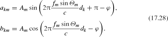
Thus the coefficients akm and bkm are time independent and for each frequency fm these coefficients represent sample values of the corresponding sinusoidal spatial signal. This analysis approach can be directly implemented on the basis of the DFT by applying DFT filter banks as shown in Figure 17.6.
This approach can also be illustrated in a slightly different way, as shown in Figure 17.7. The interpretation is based on the sensor output signal sample value matrix
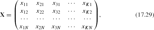
which is formed from the sample value sequences obtained by repeated sampling of the sensor output signal multitude (by taking repeated snapshots). Then the data from this matrix are used to perform DFTs in each sensor signal processing channel. The Fourier coefficients obtained in this way are later used as inputs for the spatial spectrum analysis.

Figure 17.7 Generalized outline for the DOA estimation according to which the temporal spectrum analysis is carried out first
Now the signal arrival angle Θ is considered as a variable and the time is fixed. In this case equation (17.26) can be rewritten as
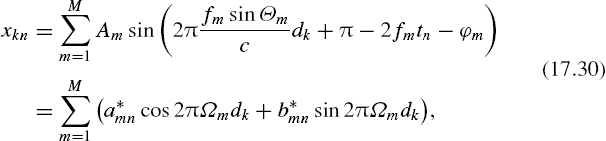
where
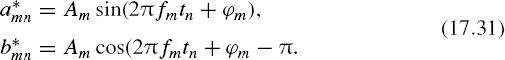
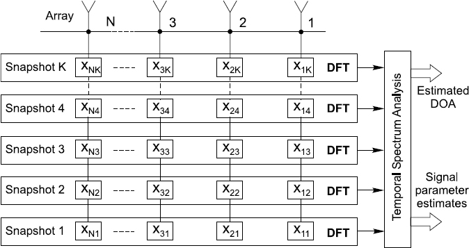
Figure 17.8 Generalized outline for the DOA estimation according to the which the DFT for the spatial spectrum analysis is calculated after taking each snapshot
It can be seen that now the coefficients a*mn and b*mn do not depend on the number of sensors. Therefore the spatial spectrum analysis, performed by processing the signal (17.30), will provide the estimates of {Ωm, a*mn, b*mn}, m = 1,..., M. On the other hand, a*mn and b*mn can be considered as signals depending on the argument tn. Note that these signals are sinusoidal. By performing a temporal spectrum analysis of them, the values of fm and Am, m = 1,..., M, are estimated. This approach to the array signal analysis is illustrated by Figure 17.8.
Consider the schemes given in Figures 17.7 and 17.8 which correspond to the cases briefly described above. It can be seen that the input data block in both cases is the same. Therefore an impression may be found that the differences between them are purely formal. However, that is not true. While the end result is indeed the same, the sequence of procedures carried out in order to obtain that result differs and so do the algorithms developed on the basis of one or the other approach. For instance, in the case illustrated by Figure 17.8, the DFT can be performed by processing the data obtained at each snapshot sequentially in time (by applying only one filter bank) while, in the case of schema given in Figure 17.7, the performance of the DFT operations is delayed until all snapshots are taken. They are then either repeated sequentially in time by one device or N such DFT devices are required to perform these transforms parallel in time for all sensor signal processing channels. The preferable approach obviously depends on the conditions under which a specific array has to function.
17.5 Pseudo-randomization of Sensor Arrays
Typically there are many sensors in the sensor arrays used in radar systems. Each of them represents a signal source and the whole multitude of signals taken off the sensors has to be processed in real time. Therefore the sensor arrays and the attached systems fulfilling the task of array signal processing are quite complicated. The problem is that they cannot be simplified without changing the very essence of the array functioning. Indeed, if, for example, the classical one-dimensional array is examined, its spatial resolution is inversely proportional to the aperture. To achieve a sufficiently high resolution, this aperture has to be large. K sensors are placed within this aperture with the distance between the sensors equal to d so that the aperture is equal to (K – 1)d. On the other hand, the minimal wavelength of array signal components is limited by the value d of the interval between the array elements. To guarantee that there is no aliasing, at least two samples from a signal wavelength should be taken, i.e. λmin ≥ 2d and Ωmax = 1/λmin. If the wavenumber of an array signal component exceeds the given limit, aliasing occurs. To satisfy both requirements of a sufficiently large aperture and small enough intervals between the sensors, the number of sensors in the array often has to be quite large and, consequently, the complexity of the array is then high.
17.5.1 Complexity Reduction of Arrays
Pseudo-randomization of the sensor array designs offers a way out of the described deadlock. Basically it is suggested that spatial aliasing can be avoided by placing sensors in the array nonuniformly. Assuming that this works, the mean distance between the sensors could then be enlarged and the number could then be significantly reduced.
This option for array complexity reduction certainly looks attractive. The question is how realistic it is. The directional pattern of a randomized array of 32 sensors is given in Figure 17.9. The first impression of the efficiency of sensor array randomization can be obtained by comparing Figures 17.4 and 17.9. It can be seen that in principle the grating lobes are indeed suppressed in the diagram in Figure 17.9. However, the obtained directional pattern of the nonuniform sensor array is clearly not very good. The question is: what is the meaning of this diagram and to what conclusions does it lead?
The well-defined aliasing taking place at functioning of the equidistant sensor arrays in the case of the nonuniform array is replaced by fuzzy spatial aliasing. The concept of fuzzy aliasing, observed at spectral analysis of signals in the time domain, is explained in Chapter 9. To put this simply, the phenomenon is caused by the nonuniformities of the intervals between signal sample value taking instants. The mean sampling rate due to these irregularities then drift in time, which leads to aliasing occurring at varying frequencies. As a result, the aliasing pattern in the frequency domain becomes fuzzy. In other words, the sharp lines indicating aliasing at definite frequencies are spread out, showing that aliasing is suppressed but occurs in a certain frequency band.
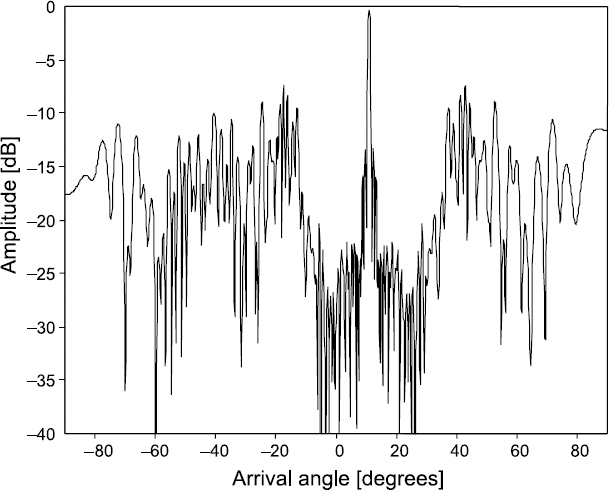
Figure 17.9 Directional pattern of a nonuniform array of 32 sensors (Θ = 11°).
Spatial fuzzy aliasing is analogous to fuzzy aliasing occurring at signal sampling in the time domain. The reason why fuzzy aliasing takes place in the spatial domain is the nonuniformity of the intervals between sensors in the array. The spatial sampling rate due to this nonuniformity is not constant, which leads to spreading out of the spatial aliasing over varying signal arrival angles.
Apparently that is not what is needed. Successful elimination of the aliasing effect really means avoiding aliasing rather than weakening it at certain frequencies and spreading the aliasing effect out into a broader frequency band. Therefore the displayed directional pattern of the pseudo-randomized array shown in Figure 17.9 should not be considered as an acceptable one.
The relatively bad results should not be surprising as they have been obtained simply by summing nonuniformly delayed spatial signal sample values. The problems encountered are similar to those observed at the DFT of nonuniformly sampled temporal signals and commented on in the introduction to Chapter 15. As soon as the sensors are placed in an array nonuniformly, the spatial signals taken off this array depend on the pattern of sensor coordinates in the array. This means that direct summing of nonuniformly delayed spatial signal sample values does not complete the process of beamforming. Obtaining this sum actually leads to the acquisition of intermediate signal processing results containing valuable information. Therefore this output signal y(t) of the phased nonuniform array considered at various signal arriving angles under these conditions should not be automatically regarded as the directional pattern of the respective array. Additionally processing of y(t) has to be undertaken with the specifics of the given sensor array nonuniformity taken into account.
A particular approach to resolution of this task is considered in Chapter 20. As shown there, adapting array signal processing to the nonuniformities of the sensor location in the array leads to much better beamforming. The directional pattern of the nonuniform array obtained as a result of such adaptation is incomparably better than the diagram displayed in Figure 17.9. This leads to the optimistic conclusion that it is possible to achieve significant complexity reduction of sensor arrays by pseudo-randomizing the array designs and performing appropriate array signal processing. The key to the success in this area is in performing effective alias-free signal processing.
17.5.2 Pseudo-randomization of Array Signal Processing
Pseudo-randomization of sensor arrays, in general, concerns both the array design (location of sensors in the array) and the array signal processing. To achieve good results at applications of the considered pseudo-randomized sensor arrays, it is crucial to ensure that processing of the signals taken off the nonuniform sensor arrays is carried out in an appropriate way. There is much in common in the approaches to temporal and spatial array signal processing.
At first glance it seems that only spatial signal processing requires development of special algorithms matched to the specifics of nonuniform sensor arrays and that processing of the temporal signals could be realized in the conventional manner. Basically this is true. On the other hand, various benefits can often be gained by also using special signal processing algorithms for handling the temporal signals. Of course, much depends on the characteristics of the signals transmitted or received by a particular sensor array. While periodic sampling and the traditional algorithms for processing temporal signals is preferable when dealing with relatively narrowband signals, the technology for alias-free signal processing discussed in this book will lead to better results in cases where the signals are wideband and/or contain components at very high frequencies.
As shown in the block diagrams of the systems used to estimate the DOA, common techniques for digital signal processing are related to the DFT performed in both domains. As a lot of attention is paid in this book to realization of these transforms, a number of the discussed techniques and algorithms are also applicable in the area of array signal processing. The nonorthogonality appearing in the basis functions used for the DFT due to irregularities of the sampling process, both in the temporal and spatial domains, might be mentioned as an example. In fact, much of the knowledge accumulated in the area of temporal signal processing could be successfully exploited for enhancement of array signal processing in the spatial domain. This is demonstrated in the next chapter, where the algorithm for adapting processing of temporal signals to the nonuniformities of sampling is modified to extend the applicability of this approach so that it can also be used for adapting spatial signal processing to the specific nonuniform pattern of sensor locations in an array. As the results obtained and displayed there show, this approach, based on the experience gained from processing temporal signals, leads to significant improvement in pseudo-randomized array performance. An example showing what can be achieved is given in Chapter 20.
As the subject of pseudo-randomized arrays is really outside the scope of this book, the brief description given here is intended to draw the attention of readers to this exciting signal processing area where many of the special alias-free signal digitizing and processing techniques considered in this book can be successfully applied.
Bibliography
Bilinskis, I. and Lagunas, M.A. (1992) Randomizing of array element spacing and of processing array signals. Submitted to the Sixth European Signal Processing Conference, Brussels, 25–28 August 1992.
Bilinskis, I. and Mikelsons, A. (1992) Randomized Signal Processing. Prentice-Hall International (UK) Ltd.
Lo, Y.T. (1964) Mathematical theory of antenna arrays with randomly spaced elements. IEEE Trans. Antennas Propag., AP-12, 257–68.
Lo, Y.T. and Simcoe, R.J. (1967) An experiment on antenna arrays with randomly spaced elements. IEEE Trans. Antennas Propag., AP-15, 231–5.
Marvasti, F. (2001) Nonuniform Sampling, Theory and Practice. New York: Kluwer Academic/Plenum Publishers.
Steinberg, B.D. (1976) Principles of Aperture and Array System Design. New York: John Wiley & Sons, Inc.