CHAPTER FIVE

Qualitative Reconstruction Methods

5.1 INTRODUCTION

In the scientific literature the term qualitative is used to denote essentially two families of reconstruction methods. In the first case it refers to approaches aimed at obtaining only some information about the scatterers under test. Such methods are generally unable to retrieve the distributions of the unknown electromagnetic parameters (e.g., dielectric permittivity, electric conductivity, magnetic permeability), but they provide information concerning only the shapes and locations of the scatterers.

In the second case, the same term is used to indicate the reconstruction methods that are based on certain approximations in scattering models (e.g., those based on Born- and Rytov-type approximations) and can then be successfully applied only if some a priori information on the unknown object is available and if the inspected objects fulfill the conditions making the approximate models valid. For example, in order to apply the Born approximation, one needs to know that the object is a weak scatterer, as discussed in detail in Chapter 4.

Despite their limited applicability, qualitative methods are of significant interest for their computational efficiency, enabling fast and robust reconstructions possible in a quite short time period. Such considerations suggest a classification of microwave imaging algorithms into two groups, namely, quantitative and qualitative methods, in order to distinguish qualitative approaches from those aimed at providing the values of the electromagnetic parameters (usually dielectric permittivity and electric conductivity) of the inspected investigation domain, without approximations on the electromagnetic model. As will appear clear from the subsequent developments discussed below, quantitative methods provide very complete information on the inspected targets, but are usually quite computationally expensive and often require a suitable starting guess of the solution in order to converge. The reader is referred to Chapter 6 for a description of this class of methods. It is worth mentioning that the above classification is highly arbitrary and other choices are possible. In particular, we note that mathematicians usually restrict use of the term qualitative only in reference to methods providing support of the scatterers (Cakoni and Colton 2006).

In the following text, we shall focus only on qualitative approaches, which are less ambitious because they either attempt to provide less complete characterization of the scatterers or can be applied only to a particular class of targets. Both the approaches are discussed. However, since many qualitative methods lead to resolution of linear ill-posed problems, in the following sections, some preliminary theory and tools useful in dealing with this class of problems are presented. In particular, the concepts of generalized inverse operators and generalized solutions are addressed, along with one of the most commonly used and powerful tools in linear inverse scattering, the singular value decomposition. Some basic concepts regarding regularization theory are also briefly introduced, without cumbersome mathematical details.

5.2 GENERALIZED SOLUTION OF LINEAR ILL-POSED PROBLEMS

As mentioned above, qualitative methods very often require the resolution of ill-posed linear problems. Some examples are represented by the linear sampling method (Section 5.8) and by the approaches based on first-order Born and Rytov approximations, described in Sections 4.6 and 4.8, respectively. However, even nonlinear methods aimed at inspecting strong scatterers can require the resolution of linear problems. An example is represented by the Newton method described in Chapter 6, in which a linearized equation is to be solved at each iteration.

In this section, we shall analyze the problem of solving the linear problem

in a quite abstract framework, since applications are described in the sections devoted to the specific inversion methods. More precisely, we shall assume that L is a linear operator between the Hilbert spaces X and Y.

In particular, we shall discuss issues related to existence, uniqueness, and continuous dependence on the data of the solution f of equation (5.2.1). With regard to existence, equation (5.2.1) admits a solution if and only if g ∈ R(L), where R(L) is the range of the operator L. If, for certain reasons (noise on the data, errors due to the measurement system, etc), g ∉ R(L), a solution does not exist in the standard sense.

On the other hand, if at least a nontrivial solution exists such that

that is, the null space (also referred to as the “kernel”) of the operator N(L) does not contain only the null element, then the solution of the equation (5.2.1) is never unique. In fact, if f is a solution, then the function f′ = f + is still a solution (for the same known term g).

As a consequence, either if R(L) is a proper subset of Y (i.e., there exists g ∉ R(L)) or if N(L) ≠ {0} [i.e., for any g ∈ R(L) there exists more than one solution of equation (5.2.1)], the problem of finding f is ill-posed, according to the definition given in Section 3.1.

Nonetheless, as will be discussed below, the standard concept of solution can be extended by introducing the generalized solution, usually denoted as f⁺, in order to resolve some nonuniqueness and nonexistence issues.

In order to define the generalized solution, it is first useful to introduce the least-squares solution (or pseudosolution) of the linear problem Lf = g. An element of X is called a least-squares solution of (5.2.1) if

or, equivalently, if it satisfies the normal form of the equation of interest, specifically

where L* is the adjoint operator of L.

In other words, a least-squares solution minimizes the norm of the residual

For this reason, it is clear that any solution of equation (5.2.1) in classical sense is a least-squares solution, too, since the residual of a classical solution is always exactly zero. However, the opposite statement does not hold true, since a least-squares solution may exist even when a standard solution cannot be found, that is, if g ∉ R(L).

On the other hand, it is worth remarking that more than one least-squares solution may exist, as the abovementioned reasoning on the kernel of L suggests. However, the uniqueness can be ensured by choosing the minimum norm least-squares solution. In fact, it can be proved that the set of least-squares solutions is a closed and convex set in X and thus always admits a unique minimum norm element (Rudin, 1970). For this reason, the generalized solution f⁺ is introduced as the least-squares solution of minimum norm.

It can also be proved that the generalized solution exists for any datum g ∈ R(L) ⊕ . where ⊕ is the direct sum operator and is the orthogonal complement of R(L) (Tikhonov et al. 1995). As a consequence, the generalized solution exists for any datum g ∈ Y if and only if the range of L is a closed set. Accordingly, the generalized inverse operator L⁺ can be introduced as an operator mapping the elements of R(L) ⊕ to the corresponding generalized solutions (Tikhonov et al. 1995) and thus it can be written

It is quite easy to verify that the generalized inverse operator is a linear operator and the generalized solution is the unique least-squares solution with no component belonging to the kernel of the operator L (Tikhonov et al. 1995). Moreover, it can be proved that the operator L⁺ is continuous when R(L) is closed in Y (Tikhonov et al. 1995). As a consequence, the problem of finding the generalized solution of a linear problem is well posed when R(L) is closed, since, in such a case, the generalized solution exists, is unique, and depends continuously on the data.

On the other hand, when R(L) is not closed, determination of the generalized solution is an ill-posed problem and regularization methods need to be introduced. Regularization theory is a wide topic that would necessitate devoting too much space in the present context for a precise description. For this reason, we shall provide only some very basic ideas.

5.3 REGULARIZATION METHODS

A regularization method consists in replacing an ill-posed problem with a well-posed problem, whose solutions approximate the one of the ill-posed problem (Sarkar et al. 1981). More precisely, the set of operators R_α, with α > 0, is said to be a regularization scheme for operator L if the following two conditions are fulfilled (Colton and Kress 1998) (where α is the regularization parameter):

1. R_α is continuous for any α > 0.
2. For every g ∈ R(L) ⊕ , R_αg − f⁺ → 0 when α → 0⁺.

In other words, regularization operators provide stable (continuous) approximations of the (unbounded) generalized inverse. It is worth noting that such a definition of regularization scheme does not involve the presence of noise.

However, the practical importance of the regularization methods is due largely to their ability to provide stable solutions even for noisy data, that is, when the known term g or the operator L are not exactly known.

In the case of noisy environments, the previously provided definition of regularization scheme needs to be slightly modified to account for the presence of noise and its level. In particular, a regularization strategy for noisy data/operators has to be equipped with a rule for the choice of the optimal regularization in dependence on noise level.

In order to clarify this point, let us assume that only the datum g is affected by noise. Then let g^δ be the noisy datum, where is δ the noise level (i.e., g − g^δ ≤ δ); it is interesting to evaluate the norm of the difference between the generalized solution f⁺ corresponding to the noiseless datum g and the quantity :

Such an inequality is very useful in understanding the effect of noise on a regularized solution. In fact, it provides an estimate of the error on the generalized solution as the sum of two terms: δR_α, which is a measure of the error on the regularized approximated solution due to the error on g; and R_αg − f⁺, which represents the approximation error due to the use of R_α instead of the generalized inverse operator. According to a definition of the regularization method, because R_αg − f⁺ → 0 as α → 0⁺ and, in ill-posed problems, R_α → ∞ as α → 0⁺, a tradeoff between the two errors is required, and it can be obtained by a suitable choice of the regularization parameter α. So it is clear that every regularization scheme requires a strategy for choosing the parameter α in dependence on the error level in order to achieve an acceptable approximation of the generalized solution.

In the scientific literature, many regularization methods have been proposed and studied. Among them, we cite the Tikhonov method, the truncated Landweber algorithm, the truncated conjugate gradient and the truncated singular value decomposition. For example, the Tikhonov method consists in minimizing the residual (5.2.5) with a penalty term. In particular, the Tikhonov regularization method is based on minimization of the functional

where the residual on the datum g is minimized along with the norm of the solution. For numerical implementation of the Tikhonov method, it is very useful to know that the function minimizing (5.3.2) is also the solution of the Euler equation

Therefore, in this case, we obtain

Other regularization methods (e.g., the truncated Landweber method) will be used in the following text and described when necessary.

Although the previously developed ideas hold true in quite general frameworks, provided that the suitable technical hypotheses are assumed, in the following text we shall address the case of finite-dimensional spaces, by introducing the singular value decomposition (SVD) of a matrix and discussing the resolution of linear problems in terms of this powerful mathematical tool.

5.4 SINGULAR VALUE DECOMPOSITION

Let us consider a generic N × M matrix [L] of complex numbers of rank p ≤ min{N, M}.

In order to introduce the singular value decomposition, let us consider, for i = 1,..., p, the vectors u_i and v_i of N and M elements, respectively, and the numbers σ_i such that

It is very easy to deduce that

As a consequence, v_i is an eigenvector of the matrix [L]*[L] with eigenvalue and u_i is an eigenvector of the matrix [L][L]*, again with eigenvalue . Since [L]*[L] and [L][L]* are both self-adjoint matrices [i.e., ([L]*[L])* = [L]*[L] and ([L][L]*)* = [L][L]*, as a consequence of well-known results in linear algebra, they are diagonalizable and all their eigenvalues are real (Bertero and Boccacci 1998). Moreover, the eigenvectors of [L]*[L] and [L][L]* can be made orthonormal in C^M and C^N, respectively. Accordingly, there exist two sequences of vectors and such that

Let us then sort the vectors and such that the corresponding eigenvalues are in decreasing order, and let us build the N × N matrix

and the M × M matrix

with the mutually orthonormal eigenvectors as columns, so that they result in unitary matrices [i.e., [U]* = [U]⁻¹ and [V]* = [V]⁻¹]. It is worth noting that, since it can be proved that the kernels of [L]*[L] and [L] coincide (Oden and Demkowicz 1996), the number of non-zero eigenvalues of [L]*[L] is equal to the rank p of [L]. On the basis of the pointed out properties and equations (5.4.5) and (5.4.6), we can then write

Equations (5.4.9) and (5.4.10) can be expressed in a compact form by using matrices [U] and [V] as

where [Σ] is the N × M real matrix given by

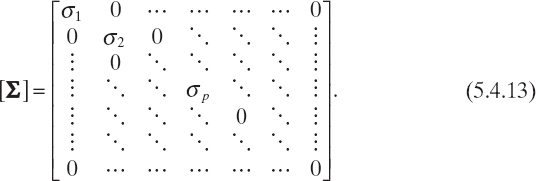
In the following paragraphs, it will be useful to define σ_I = 0 for i = p + 1, ..., M.

Since [V]* = [V]⁻¹, from equation (5.4.11) it immediately follows that

which is called the singular value decomposition of the complex matrix [L]. The diagonal elements of [Σ] are called the singular values of the matrix [L], and there are exactly p nonzero singular values. Moreover, the columns of [U] and [V] are called the singular vectors of the matrix [L]. The whole composite of singular values and singular vectors of [L] is referred to as the singular system of [L].

Of course, as [Σ] is a matrix of real numbers, a similar decomposition for the adjoint matrix [L]* can be provided as follows:

Equations (5.4.14) and (5.4.15) are rich in consequences. In fact, since the singular vectors and are mutually orthonormal in C^N and C^M, respectively, is a orthonormal basis in C^N and is a orthonormal basis in C^M. More precisely, is an orthonormal basis for the orthogonal complement of the kernel of [L], whereas is an orthonormal basis for the kernel of [L] (Oden and Demkowicz 1996). Analogously, is an orthonormal basis for the orthogonal complement of the range of [L], whereas is an orthonormal basis for the orthogonal complement of the range of [L].

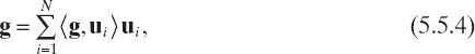
As a consequence of this important property, the image of any element of C^M through [L] can be expressed by means of its singular system. In fact, as f is a generic element of C^M, it follows that

and, since are mutually orthonormal in C^M, we obtain

As a consequence

Moreover, using the mutual orthonormality of the elements of , we obtain

Because σ₁ ≥ σ₂ ≥ ··· ≥ σ_p > 0, from equation (5.4.19) and (5.4.17), where p ≤ M, we deduce that

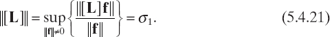
It is worth remarking that the equality can hold true in (5.4.20) when f has a nonzero component only along the first singular vector v₁. Accordingly, the standard norm [L] of matrix [L] can be easily expressed in terms of its maximum singular value, by observing that

5.5 SINGULAR VALUE DECOMPOSITION FOR SOLVING LINEAR PROBLEMS

Singular value decomposition (SVD) also plays an important role in the resolution of linear problems, and this is the main reason why it is presented in this book. In order to explain this point, let us consider the system of equations

and let us look for its generalized solution, that is, for a vector f such that

To this end, it is useful to observe that, by using (5.4.18), we can write

Moreover

and hence

Using (5.5.3) and (5.5.5), we can rewrite equation (5.5.2) as

or, equivalently, because the singular vectors are mutually orthonormal, as

As a consequence, a solution of (5.5.2) is given by

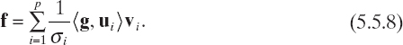
Since the vectors are an orthonormal basis for the orthogonal complement of the kernel of [L], the solution (5.5.8) has no component in the null space of [L] and so, as observed above in a more general setting, it is the generalized solution of the linear problem (5.5.1):

In such a way, we have shown that the generalized solution of the generic linear system (5.5.1) can be explicitly expressed by means of the SVD of the matrix [L].

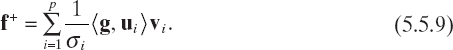
Equation (5.5.9) is also very useful, since it readily provides the generalized inverse matrix [L]⁺ referred to also as the pseudoinverse matrix. In fact, on the basis of the general theory described in the previous section, we can write

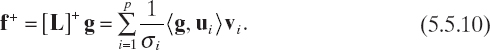
As a consequence

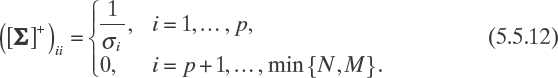
where [Σ]⁺ is a N × M diagonal matrix, with diagonal elements given by

From (5.5.11) it easily follows that

It should be noted that the use of the pseudoinverse solution can solve uniqueness and nonexistence problems, but numerical instability may still affect the computation of f⁺. In practice, we mean that, although (5.5.10) always holds true, large numerical errors may occur on f⁺ even if the datum g is affected by small errors.

In order to make these considerations more precise, let us consider the datum g to be affected by an error δg, that is, only the “noisy” version

of g is disposable, and let us evaluate the impact of this error on the corresponding generalized solution f^+,e. Since

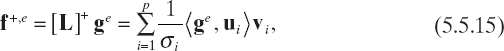
from (5.5.10), it follows that

As a consequence, we have

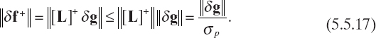
Moreover, from (5.5.10) it follows that

where g _r([L]) denotes the projection of g onto the range of the matrix [L]. Therefore, from (5.5.18) and (5.5.17) it follows (for f⁺ ≠ 0) that

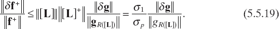
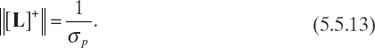
From equation (5.5.19), it is easily deduced that the relative error on the known term corresponds to a relative error on the generalized solution that is controlled by the quantity

which is called the condition number of the matrix [L]. It is worth observing that, since σ₁ ≥ σ_p, it follows that m ≥ 1.

The condition number indicates the sensitivity of the solution with respect to the error on the known term and depends on the ratio between the largest and the smallest singular values of [L]. From equation (5.5.20), we see immediately that if m is small, small changes in the known term will result in small variations in the solution, otherwise, small changes in the data will result in large variations in the solution. In the former case, the discrete problem (and the related matrix) is said to be well-conditioned, in the latter case, it is said to be ill-conditioned. Unfortunately, the discretization of ill-posed inverse problems usually leads to systems of equations characterized by very high condition numbers. Moreover, the finer is the discretization of the continuous ill-posed problem, typically the higher is the condition number of the resulting matrix. This can be explained by observing that a finer discretization produces a better approximation of the continuous operator, whose inverse is usually unbounded. This should be carefully accounted for in practical applications, where a tradeoff between resolution (high resolution would require a fine discretization) and stability (coarse discretization) must be pursued.

Consequently, the linear systems occurring in the resolution of inverse problems suffer from a severe numerical instability. For example (Bertero and Boccacci 1998), if m = 10⁶, a small error in the data of the order of 10⁻⁶ could result in an error in the solution of the order of 100%.

On the other hand, to be thorough, it should also be mentioned that discretization of a direct scattering problem usually results in a well-conditioned matrix to be inverted, as a result of the usual well-posedness of the continuous direct model.

5.6 REGULARIZED SOLUTION OF A LINEAR SYSTEM USING SINGULAR VALUE DECOMPOSITION

The singular value decomposition is very useful also because it allows a direct expression for the Tikhonov regularized solution of the linear system (5.5.1). To achieve this goal, let us consider the Euler equation [see equation (5.3.3)] for the Tikhonov solution of the linear system (5.5.1), which reads as

Since the solution is an element of C^M, it can be expressed as a linear combination of singular vectors as in equation (5.4.16). Moreover, by using equation (5.5.5), it follows that

Since

it follows that

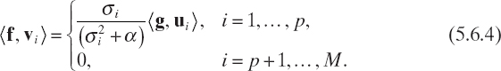
The Tikhonov regularized solution can then be written as

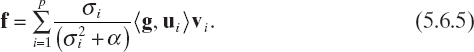
Another commonly used strategy to regularize the solution of ill-conditioned linear systems consists in the so-called truncated singular value decomposition (TSVD). The basic idea is to neglect the smallest singular values of the involved matrix, in order to reduce the condition number. Of course, a tradeoff between stability and accuracy must be found. More precisely, if σ_p′ > σ_p (p′ < p) denotes the smallest considered singular value, the related solution is given by

The corresponding error on the fitting of the known term can easily be deduced as

It is worth remarking that the choice of p′ is often a critical issue, as well as the selection of α for the Tikhonov regularization, and the optimal choice is not at all an easy task (Caorsi et al. 1995). In fact, an estimation of the noise level is often required for selection of the optimal value, and several approaches have been proposed in the literature. One of the most commonly adopted strategies is based on the Morozov principle (Colton and Kress 1998), which stipulates that the value of α selected must ensure that the error on the retrieved solution is of the same level as the error on the data. This is a reasonable criterion that is often used in practical applications in which a noise-level estimation is available; for instance, the rule used to choose the value of the regularization parameter in the linear sampling method described below, is based on the Morozov principle.

5.7 QUALITATIVE METHODS FOR OBJECT LOCALIZATION AND SHAPING

Several different methods can be applied to localize an unknown scatterer and define its shape. Among them we can mention the linear sampling method and the level-set method. These methods have been widely studied in the scientific literature, and the reader is referred to the references cited in the following sections. Formulation of the linear sampling method will be outlined in the following section, since this technique is one of the most used, not only as an independent qualitative procedure (with intrinsic computational efficiency) but also in conjunction with quantitative techniques. This important aspect will be discussed in Chapter 8.

A further consideration is necessary. As clearly specified in the previous chapters, this book essentially focuses on short-range imaging techniques. However, it is not possible to set a precise bound for the set of considered techniques based on the distance between the illuminating/receiving elements and the target under test, since, for example, some radar techniques are used in both near-field and far-field ranges. At the same time, some common tomographic methods, which, of course, imply the possibility of sensing the scattered field around the target, in certain frequency ranges, still assume far-field operation conditions, and plane waves are used (at least as approximations) for illumination purposes. The choice of the author is to consider techniques that have been proposed for engineering applications in which the imaging system must be positioned at a relatively short distance, in the common sense, to the object or apparatus to be inspected.

5.8 THE LINEAR SAMPLING METHOD

A method for rapid determination of the shape of a scattering object is the so-called linear sampling method (Colton and Kress 1998, Cakoni and Colton 2006, Colton et al. 2003). Under the assumption in Section 3.3 for two-dimensional inverse scattering, we consider the inspection of an inhomogeneous object of support S_o starting from knowledge of the field that it scatters in the far-field region. Moreover, the object is assumed to be illuminated by a set of uniform plane waves, although this is not a strict requirement, since the linear sampling method can be extended to other incident fields and near-field measurements (Colton and Monk 1998). According to equation (2.4.24), we assume again and the propagation vector given by equation (3.5.1).

The scattered electric field admits the asymptotic behavior given by

where . Equation (5.8.2) is clearly the two-dimensional counterpart of equation (2.4.22). The scalar field E_∞z is often called the far-field pattern in the scientific literature on the linear sampling method (Cakoni and Colton 2006). Since the scattered field E_scatz depends on the incident field, so does the far-field pattern. Consequently, the angle of incidence can be made explicit by writing E_∞z = E_∞z. The starting relation of the linear sampling method is the following integral equation (Colton et al. 2003)

where the unknown g is a complex function that, for any z_t, belongs to L²(0,2π), and is given by

which, in the preceding notation, represents the far-field pattern of the Green function of the background along direction , when the impulsive source is located at point z_t. Equation (5.8.2) is a Fredholm linear integral equation of the first kind [see Section 3.1 and equation (3.1.1)].

The importance of such an equation is due to the fact that it admits an approximate solution g, whose norm blows up near the boundary of the scatterer and remains large outside; in such a way it is possible to exploit it to visualize the support of the inspected scatterer (Cakoni and Colton 2006).

In real experiments, since the far-field pattern can be measured for only a finite number S of incidence directions and a finite number M of measurement directions (see Section 4.3), equation (5.8.2) needs to be discretized. To this end, a M × S matrix [L] is introduced whose (mj)th element l_mj is the far-field pattern along the mth observation direction when the incident field is a plane wave of incidence angle . For the sake of simplicity, the incidence and the observation directions will be assumed to be uniformly spaced, i.e., = (2π/S)(j − 1), j = 1,..., S, and = (2π/M)(m − 1), m = 1,..., M [see equations (4.3.6) and (4.3.10)].

In a discrete setting, for a fixed z_t, the far-field equation then becomes

Here, denotes a vector of M elements, whose entries , m = 1,..., M, are the far-field values of Green's function along the directions m = 1,..., M, when the implusive source is placed at the point z_t, that is, , m = 1,..., M. The term is a vector of size S containing the values of the unknown function at the incidence directions: , j = 1,..., S.

Moreover, in practice, the far-field pattern E_∞z cannot be known exactly; only noisy measurements of it are available. As a consequence, the datum actually at disposal is the noisy far-field pattern . Accordingly, [L] is replaced with [Lⁿ]. Moreover, since equation (5.8.2) is ill-posed, its discrete counterpart is ill-conditioned, and a regularization scheme, requiring a regularization parameter, is needed to solve it.

In summary, the linear sampling method can be described as follows:

1. Choose a grid of points Z ⊂ , containing the scatterer and for each point z_t ∈ Z.
   1. Find a one-parameter family of regularized solutions of equation (5.8.4), where α(z_t) denotes the regularization parameter related to the equation holding for z_t.
   2. Find the optimum regularization parameter α*(z_t) and the related solution , according to an optimality criterion.
   3. Store the norm of the optimum solution.
2. Choose a monotonic function , called the indicator function, and, for each point of the grid Z, plot the composite function of the position .

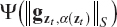Following the literature on the linear sampling method, in the sequel the regularized solution of the equation (5.8.4) is determined by using the Tikhonov method (Tikhonov et al. 1995), which has been described in Section 5.6. Moreover, since the noise affects the matrix of coefficients of the linear systems (5.8.14), the optimal regularization parameter is selected by using the Morozov discrepancy criterion (Tikhonov et al. 1995).

For each z_t ∈ Z, the Tikhonov regularized solution of the equation (5.8.4) of regularization parameter α(z_t) is such that

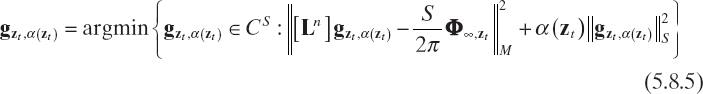
If the singular value decomposition (Section 5.5) of the [Lⁿ] matrix is performed, can then be expressed as

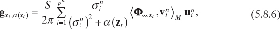
where is the standard scalar product in C^S, pⁿ is the rank of the matrix [Lⁿ], and is its singular system. Moreover, since the singular vectors are orthonormal, it follows that

Selection of the optimal regularization parameter requires an estimate of the noise level. Such an estimate can be given in terms of the positive real number h such that [Lⁿ] − [L] < h. Accordingly, the generalized discrepancy principle (Tikhonov et al. 1995) used for determining the optimal regularization parameter requires that α*(z_t) be the zero of the generalized discrepancy

Using (5.8.6) and the properties of the singular value decomposition, we can easily prove that

Clearly, the key aspect of the approach is essentially the search for a given set of “amplitudes” (the values of g_zt,) for the incident plane waves so that their combined effect is such that the induced currents on the unknown target are able to generate a symmetric scattering pattern. Since this pattern can be achieved only when the scatterer is a point scatterer or occupies a very small volume, the solution g_zt corresponds to a set of illumination amplitudes (one for each value of φ_inc) such that the incident field is focused on a point or in a small zone of the scatterer. In this case, only this zone essentially contributes to the scattering phenomenon. Moreover, since a regularized solution is searched for, this means that such a distribution of amplitudes for the incident fields is found only approximately, and this equivalent beamforming approach concentrates approximately the field in a single point. It should also be noted that the induced current (acting as required) can exist only inside the scatterer, whereas outside it, only incident fields with infinite amplitudes can produce a finite induced current, where the object function is equal to zero [equation (2.6.10)].

It should also be mentioned that, in a discrete setting, since only a finite number of incident directions S can be used to illuminate the target and a fixed number of measurement directions M can be considered, a rule for choosing such parameters is very useful. For the two-dimensional case, it has been estimated (Catapano et al. 2007) that good shapes can be reconstructed if

where a is the radius of the minimum circle that can include the object cross section.

For illustration purposes, let us consider a numerical example. Figure 5.1 shows the cross section of an infinite homogeneous elliptic cylinder. The semimajor axis of the ellipses is a = 0.75λ, where λ is the free-space wavelength of the monochromatic incident fields; the semiminor axis is b = 0.375λ; and the eccentricity is ≈ 0.87. The cross section center coincides with the center of the investigation area (Section 3.2), which is a square domain of side d = 2λ. The background is a vacuum (ε_b = ε₀), whereas the homogeneous cylinder is characterized by ε = (1.8 − j0)ε₀.

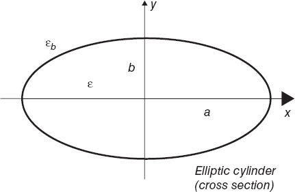
FIGURE 5.1 Cross section of an infinite homogenous lossless dielectric elliptic cylinder. Major axis: a = 1.5λ. Minor axis: b = 0.75λ. Propagation medium: vacuum (ε_b = ε₀).

According to the tomographic configuration described in Section 4.3, the object is successively illuminated by S = 36 unit plane waves with incident angles equally spaced. Measurements of the total electric field are performed on a circumference of radius ρ_M = 100λ. On this circumference, M = 36 measurement points are equally distributed; that is, the measurement points have polar coordinates such that φ_m, m = 1,..., M, is as given by (4.3.10). The total fields at the measurement points are analytically computed by using the eigenfunction expansions in terms of Mathieu functions (see Section 3.5). Then, by subtracting the values of the incident fields, the samples of the scattered fields are calculated.

In order to simulate realistic imaging conditions, the obtained values , i = 1,..., S, m = 1,..., M, are corrupted by added noise, that is

where the values N_mi are the realizations of a Gaussian process with zero mean values and variances corresponding to a fixed signal-to-noise ratio (SNR). The used indicator function is B, where A (>0) and B are constants such that belongs to the range [0,1].

Figures 5.2a–h show the reconstructed shapes of the elliptic cylinder for input data with noise levels ranging from SNR = 5 to 30dB. The figures also report the retrieved shapes obtained as the set of points where the indicator function exceeds a prefixed value. In these cases, such a threshold for the normalized indicator function has been selected to be equal to 0.64 by minimizing the reconstruction error in a reference configuration.

The investigation area is a square of dimension 2λ × 2λ, which is partitioned into 127 × 127 pixels. As can be seen, for higher values of SNR the shape of the object is retrieved quite accurately (no interpolations are used in constructing the final profile), whereas even for low SNR values the object is correctly localized inside the investigation domain, but the shape is retrieved only approximately. In order to evaluate the errors in localizing the cross section, a simple parameter has been used, which is defined as the ratio between the grid points correctly attributed to the scatterer or to the background and the total number of points. Table 5.1 provides the percentage values of such an error parameter. From a computational perspective, each reconstruction required a central processing unit (CPU) time of ∼8s on a 3 GHz Pentium PC, with a 1-GB random-access memory (RAM). Finally, as mentioned earlier, it should be noted that the linear sampling method is only one of the qualitative techniques able to provide the shapes of unknown scatterers. Another widely applied approach is based on the so-called level set method, for which the reader is referred to the literature (Litman et al. 1998, Berg and K. Holmstrom 1999, Dorn et al. 2000, Burger 2001, Ramananjaona et al. 2001, Ferraye et. al. 2003, Burger and Osher 2005, Litman 2005, Alexandrov and Santosa 2005, Dorn and Lesselier 2006, Hajihashemii and El-Shenawee 2008 and references cited therein).

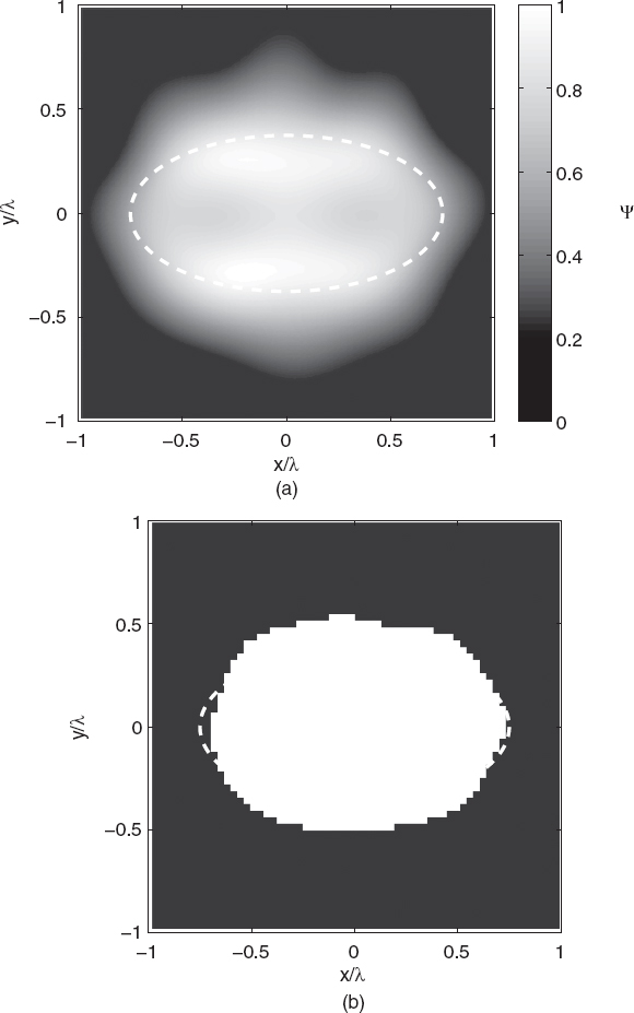
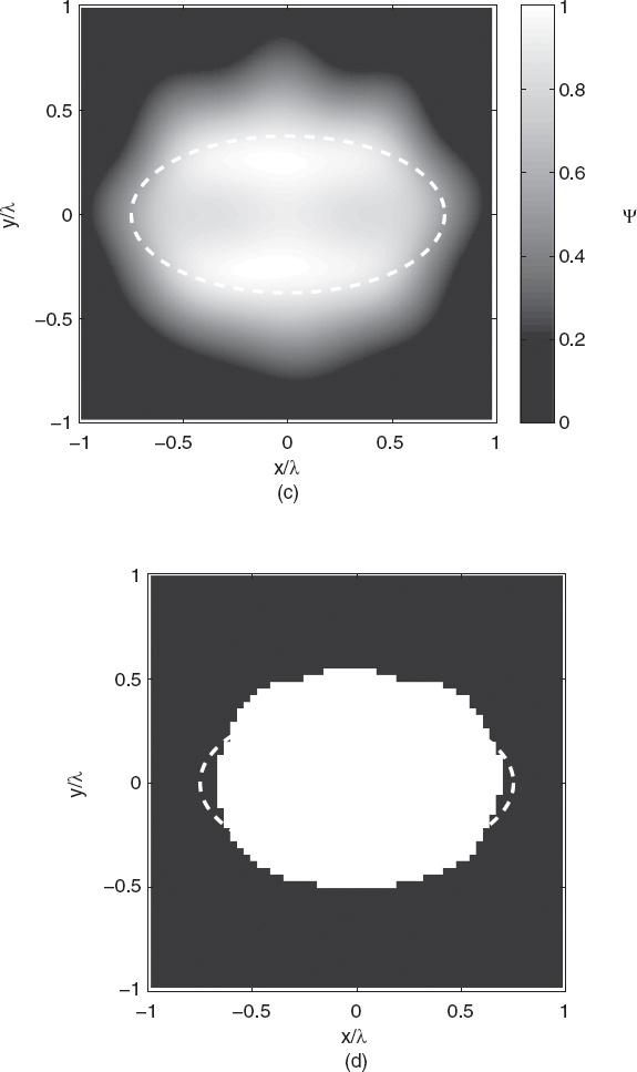
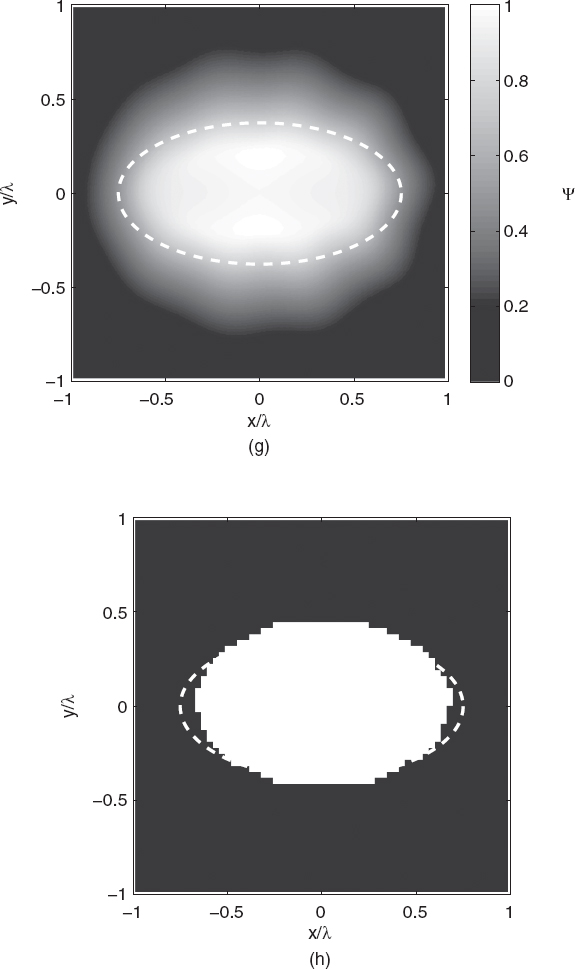
FIGURE 5.2 Shape retrieval of the homogenous lossless elliptic cylinder shown in Figure 5.1 (cross section) using linear sampling method. Plane-wave illumination (S = 36, M = 36 measurement points on a circumference of radius 100λ). Square investigation domain (side: d = 2λ; discretization: 127 × 127 pixels). Complex dielectric permittivity: ε = (1.8 − j₀)ε₀. Retrieved profiles [(a), (c), (e), (g)] and shape functions [(b), (d), (f), (h)]. Gaussian noise: (a), (b) SNR = 5dB, (c), (d) SNR = 10dB, (e), (f) SNR = 20dB, (g), (h) SNR = 30dB. The dashed line in each plot indicates the original profile.

TABLE 5.1 Percentage Error on Reconstruction of Shape of Elliptic Cylinder in Figure 5.1 for Different Noise Levels on Data Using the Linear Sampling Method

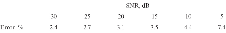
Source: Simulations performed by G. Bozza, University of Genoa, Italy.

5.9 SYNTHETIC FOCUSING TECHNIQUES

Very interesting results in microwave imaging applications have been obtained by using synthetic focusing techniques based on beamforming methods applied using the imaging configurations shown in Figures 4.6 and 4.7. These techniques are not really based on the “inversion” of the data as described in the previous chapters; thus they are mentioned only briefly here, and the reader is referred to the specialized publications cited in the present paragraph.

Synthetic focusing methods are based on the concept of synthetic aperture radar, which is widely used in remote sensing applications. Essentially, the target is illuminated by a single antenna that assumes successively different positions (Fig. 4.6). At each position, the antenna transmits a microwave signal and receives the echo (reflected signal). The echoes are not used directly. On the contrary, they are converted in discrete form and stored. When a sufficient number of measurements have been performed, the measured signal are summed after a proper time (or phase) shifting. If the shifting is correctly performed, only the reflected signal arriving from a reduced zone (ideally, a point scattering) contributes constructively to the sum. On the contrary, the scattered signals due to the other zones of the scatter add destructively, and their contributions can be considered as noise in the measured data. This measurement modality synthesizes an array antenna, in which several transmitting/receiving elements work simultaneously (with great improvement with respect to the single element in terms of gain and beamwidth reduction, resulting in very high spatial resolution). Synthetic techniques are an alternative to the use of a real array (Fig. 4.7), since they are far less expensive and do not require complex feeding circuits and multiplexing approaches. Mutual coupling among elements is also avoided, although the acquisition time can be much higher. Moreover, a mechanical system for the probe movements is necessary.

An example of this class of methods is constituted by ultrawideband techniques more recently explored mainly, but not exclusively, for medical applications. These techniques seldom attempt to reconstruct the complete profile of the dielectric properties of the region of interest, but instead seek to identify the presence and location of targets by their scattering signature.

In a basic time-domain formulation, the ultrawideband transmitter radiates bursts of radiofrequency (RF)/microwave energy of extremely short duration (tens of picoseconds to nanoseconds). The energy is scattered by discontinuities present inside the propagation medium. As mentioned, the scattered waves are collected by one or more receiving antennas (Li et al. 2005). Since, by proper combination of the receiving signals, one is able to obtain the response of a very limited zone inside the scatterer, one can construct an image of the reflection property of the target by successively exploring, pixel by pixel, the whole target. This can be done simply by changing the shifting values added to the received signals at the various measurement positions of the scanning probe. The main difficulty inherent in this simple approach is that, for focusing on a specific space point, the various shifting coefficients need to be defined with knowledge of the propagation velocity inside the propagation medium. However, since the wave velocity inside the target to be inspected (which is unknown) is not known, some a priori information can be used in this case, too (e.g., a reasonable estimate of the velocity in a model of the target under test must be assumed).

The basic formulation can be improved in the light of its application to specific cases (e.g., in medical imaging or nondestructive evaluations). First, there is the need for compensating for the reflection due to the external boundaries of the scatterer under test. In some cases, the external shape of the object is known and, consequently, from the distance between the interface and the probes one can deduce which part of the reflected signal is to be eliminated. In other cases, however, this distance is not known. For example, in medical imaging, where there is the need to compensate for the reflection from the air–skin interface, the shape of the body is patient-dependent. Consequently, specific procedures must be developed to deduce the first reflection from the target.

Another important issue concerns the compensation of dispersion effects in the signal propagation, which can introduce notable broadening in the pulse duration. In medical applications, an approach based on a broadband beam-former implementing frequency-dependent amplitudes and phase changes in the various channels has been presented (Li et al. 2005). Such approaches of can be implemented both in frequency and time domains (Bond et al. 2003, Chen et al. 2007, Mohan and Yang 2009). However, since the scientific literature on beamforming and synthetic aperture methods is wide, no further details are given in the present book, and the reader is referred to the cited papers. Some other key references will be provided in Section 10.2.

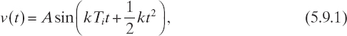
In general, for the microwave imaging techniques considered so far, including the synthetic focusing techniques, the scattering phenomenon is clearly the fundamental element. However, some other approaches have been developed that try to consider the scattering phenomenon as a disturbing effect to be possibly removed. One of them is based on the use of a chirp radar (Bertero et al. 2000). In this technique a transmitting antenna and a receiving antenna are located on different sides of the object to be inspected (see Fig. 4.5). The transmitting antenna is excited by a chirp pulse given by

where T_i and k are parameters to be chosen by the user (Bertero et al. 2000). In constructing the image of the object cross section (cylindrical objects are inspected), only the straight path between the two antennas is considered. This path is distinguished from the others by the fact that the frequency of the beat signal between the input chirp pulse signal and the output signal is determined by the time delay between the two signals. The transmitted wave component on the straight path is extracted by measuring the intensity at the frequency corresponding to the straight line between the two antennas. The key idea is to extract only the signal transmitted on a straight path in order to apply simple back projection algorithms, which are used, for example, in X-ray computerized tomography and, in general, in those imaging techniques for which the assumptions of ray propagation are valid.

It should be noted that the same approach has also been proposed with respect to a backscattering configuration, in which both the transmitting and receiving antennas are located on the same side of the object to be inspected. In this case the receiving signal is essentially a reflected signal.

5.10 QUALITATIVE METHODS FOR IMAGING BASED ON APPROXIMATIONS

According to the discussion on the meaning of qualitative reconstruction methods adopted in this book, this section is devoted to a description of algorithms that are referred to as qualitative, since they are based on scattering models involving some approximations, such as those presented in Chapter 4. In particular, the most interesting methods that are described here are the diffraction tomography (Section 5.11) and Born-like methods (Sections 5.12 and 5.13).

It should be noticed that Born approximations of order higher than 1 lead to nonlinear problems, which may require iterative resolution methods. Incidentally, the distinction between linear and nonlinear scattering models is another largely used criterion in inverse scattering literature to classify inversion approaches (Pike and Sabatier 2001).

5.11 DIFFRACTION TOMOGRAPHY

Diffraction tomography (DT) can be seen as an extension to scattered waves of the well-known computerized technique based on Radon transform and valid for X rays. Accordingly, diffraction tomography applies to two-dimensional problems, and the hypothesis of transverse magnetic (TM) illumination will be adopted (Bolomey et al. 1982, Devaney 1983, Pichot et al. 1985).

Moreover, according to the assumptions made in Chapter 4 concerning the imaging configurations, here the scattered field is supposedly collected along a straight probing line, located at distance Y₀ from the origin of the frame and completely outside the investigation domain S_i. Moreover, let φ be the angle between the probing line and the x axis of the reference frame.

The integral equation governing the scattering phenomenon can be written as follows [see equation (3.3.8)]:

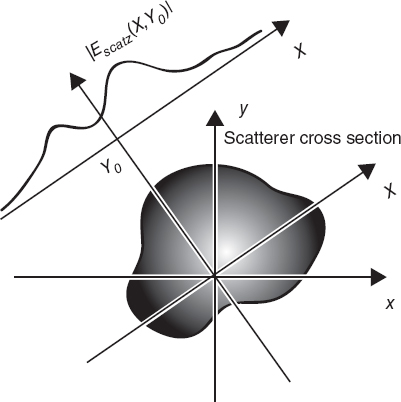
FIGURE 5.3 Two-dimensional imaging configuration for transmission diffraction tomography.

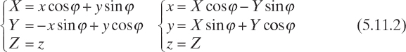
It is then very useful to introduce a new reference frame wherein the probing line is parallel to one of the coordinate axes. This goal can be achieved by means of the reference frame of Cartesian coordinates (X,Y,Z) and position vector R = R_t + (see Fig. 5.3), such that

In this new frame, the probing line is expressed by the equation Y = Y₀, and we obtain

where and denote the scattered field and the equivalent current in the rotated framework, respectively.

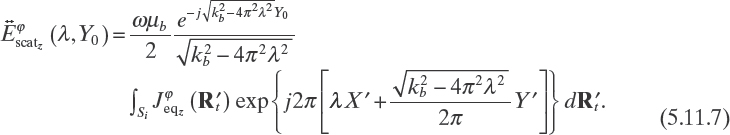
By using the plane-wave representation for the free-space Green function [equation (3.3.10)], and since Y₀ > Y′, for every Y′ ∈ S_i, because the probing line is outside the investigation domain, one obtains

In terms of its Fourier transform with respect to X, the scattered electric field collected along the probing line of equation Y = Y₀ can be written as

whence, using (5.11.4), it follows that

that is

By considering the two-dimensional Fourier transform of the equivalent current density

with K_t = , we obtain

with κ(λ) = . Since [see equation (5.11.2)]

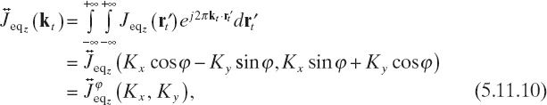
with k_t = , from (5.11.9) and (5.11.10) we have

where

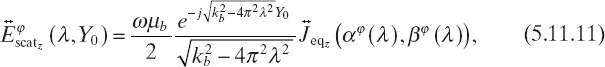
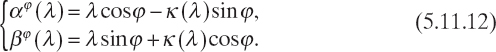
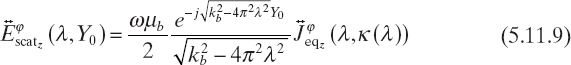
Equation (5.11.11) is the key relation of diffraction tomography and states that the one-dimensional Fourier transform of the z component of the scattered electric field measured along a straight probing line is equal to the two-dimensional Fourier transform of the equivalent current density computed along a line of the transformed plane whose parametric equation is given by (5.11.12), which turns out to be an arc of circumference.

Equation (5.11.11) represents the Fourier diffraction theorem, which is in a certain sense a generalization of the Fourier slice theorem for tomographic approaches based on straight propagation (ray propagation), in which the projection collected in a given point of the probing line depends only on the perturbation introduced in the incident wave by the body along the straight path followed by the incident wave (inside the body) to reach that measurement point.

It should be noted that the approach followed here in deriving equation (5.11.11) is the most intuitive. However, an expression for the same Fourier diffraction theorem can be deduced by a direct computation of the Fourier transforms in equation (5.11.1) (Kak and Slaney 1988).

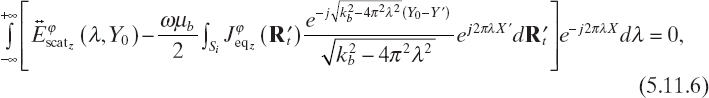
Equation (5.11.11) can be used to obtain and hence J_eqz. The problem is that different arcs of circumferences need to be combined in order to fill the frequency plane and obtain the necessary information. This can be done in several ways. The simplest one consists in rotating the illumination and measurement system around the object. It should be noted that this is essentially equivalent to keeping the imaging system fixed and rotating the object around its center.

It is clear that a perfect reconstruction can be obtained only if the two-dimensional Fourier transform of the equivalent current density is bandlimited. For objects with limited cross sections, since J_eqz (r_t) is bounded [i.e., J_eqz(r_t) = 0 for r_t ∉ S_i], it follows that is unbounded. Consequently, only a bandlimited version of the original can be recovered by using the diffraction tomography, although it has been argued that “in practice, the loss of resolution caused by this band-limiting factor is negligible, being more influenced by considerations such the aperture size of transmitting and receiving elements, etc.” (Kak and Slaney 1988 p. 234).

Actually, other practical issues have to be considered. First, the probing line cannot be infinite in extent. This means that a windowed version of the measured values along the probing line is available, namely

where l is the length of the probing line. This is equivalent to multiplying the first side of equation (5.11.5) by a rectangular window function centered at X = 0 and of width l. Accordingly, the computed Fourier transform results to be convoluted with a sinc function

where * denotes the usual convolution operator. According to (5.11.14), th e limited probing line results in another approximation on the retrieved (k_t).

Furthermore, in a discrete setting, the scattered field is measured in a finite set of points. Consequently, the Fourier transforms described above are substituted by discrete Fourier transforms (DFTs) and the is consequently available on a grid in the transformed plane.

At the same time, the discretized version of equation (5.11.11) allows for the use of fast Fourier transforms (FFTs), making the approach extremely fast and effective.

In addition, the previously discussed bandlimitation has another important consequence; specifically, the spatial resolution of diffraction tomography is limited by (Pichot et al. 1985)

This limit is particularly significant in microwave imaging, since it indicates that a limited spatial resolution can be obtained at these frequencies by using this technique. Such a resolution is not comparable with the one obtained by using other diagnostic systems working in different bands of the electromagnetic spectrum (e.g., X rays).

It should be noted that the limited spatial resolution of diffraction tomography and its applicability to weakly scattering objects only has been the main reason leading to the exploitation of quantitative approaches (described in Chapter 6), which, in principle, can be applied to strong scatterers because they are not based on approximations different from numerical ones and exhibit spatial resolution theoretically independent of the operating frequency. Furthermore, it is quite difficult to introduce a priori information on the target to be inspected into the diffraction tomography scheme.

It should also be realized that diffraction tomography only reconstructs the distribution of the equivalent current density, which usually provides limited information about the scatterer cross section (see also Section 5.14). However, for weakly scattering objects for which the first-order Born approximation can be applied, the internal electric field is approximated with the incident one and the dielectric properties of the inspected scatterer can be retrieved from the equivalent source. Nevertheless, since diffraction tomography is very simple to implement, it can provide good images of weakly scattering bodies and can also be used as initial guesswork for quantitative reconstruction methods (Franchois et al. 1998).

It should also be noted that, in the scientific literature, a different approach has been developed starting from the Rytov approximation (Devaney 1986), and higher-order versions of diffraction tomography have been proposed as well (Tsihrintzis and Devaney 2000).

Finally, as mentioned at the beginning of this section, diffraction tomography can be essentially seen as an extension of computerized tomography. Concerning this point, it should be mentioned that methods essentially based on geometric ray tracing, which are valid for ray propagation as in the case of X rays, have also been proposed for microwave imaging. Multiple scattering is neglected and the field at a receiving point is assumed to be essentially a perturbed version of the field emitted by a source on the other side of the object, where the perturbation is due to the dielectric properties of the object along a straight line that corresponds to a ray connecting the transmitting and receiving antennas. By rotating sources and receiving elements, numerous measured values can be collected for use as input data for simple reconstruction procedures. An example of these approaches is represented by the algebraic reconstruction technique (ART), which has been successively modified in order to partially account for the scattering phenomenon, in particular, the scattering effects due to parts of the scatterer adjacent to the internal region targeted by the ray propagation. The reader is referred to studies by Maini et al. (1981) and Datta and Bandyopadhyay (1985) and to the references cited therein for further details on these simplified (and fast) methods.

5.12 INVERSION APPROACHES BASED ON BORN-LIKE APPROXIMATIONS

Under the first-order Born approximation, equation (3.3.8) reads as

which is a linear equation in the only unknown τ, since the incident field is known everywhere. This is an example of a linear inverse problem, generically expressed by a linear functional equation of type Lf = g [equation (3.1.1)]. Consequently, the following considerations are valid for a large class of inverse problems not necessarily related to microwave imaging.

Let us consider now the discretization of equation (5.12.1), Following the same approach used in Section 3.4 and with the same choice of basis and testing functions, after some trivial steps, one obtains an equation similar to (3.4.5), specifically

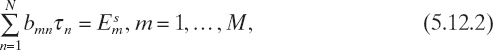
in which the coefficients b_mn are given by

[compare with equation (3.4.6)]. Moreover, the known terms are still given by equations (3.4.7). The algebraic system of linear equations (5.12.2) can be rewritten in matrix form as

where e^s = , and b_mn is the element of the mth row and nth column of the N × M matrix [B].

The linear system (5.12.4) is obtained as the discrete counterpart of a Fredholm integral equation of the first kind, and thus is usually ill-conditioned. For this reason, it needs to be solved with care, and the truncated singular value decomposition (Section 5.6) is often the tool used to obtain a stable solution with respect to noise.

To give the reader an idea of the reconstruction capabilities of the truncated singular value decomposition applied to equation (5.12.4), the reconstruction of the homogenous elliptic cylinder of Figure 5.1 is considered again. In this case, with reference to the tomographic configuration described in Section 4.3, the object is successively illuminated by S = 8 line-current sources equally spaced on a circumference of radius ρ_S = 1.5λ. The incident field generated by these sources is then given by equation (4.3.7), with , where φ_i = (2π/S)(i− 1), for i = 1,..., S. The measurements of the total electric field are performed on a circumference of radius ρ_M = ρ_s. On this circumference M = 55 measurement points are located on an arc corresponding to an angular sector of 270° in the opposite part of illuminating source; that is, for the ith source the measurement points have polar coordinates , such that

The total electric field at the measurement points (near-field line-current scattering) is computed analytically (Caorsi et al. 2000). Then, by subtracting the values of the incident fields, the samples of the scattered fields are calculated and corrupted by additive Gaussian noise [equation (5.8.11)]. In particular, for this simulation, we assumed values of the signal-to-ratio ranging from 5 to 50 dB. Furthermore, the investigation area is partitioned into 30 × 30 square pixels.

Figures 5.4a–d show the reconstructed distributions of the relative dielectric permittivity. As can be seen, due to the weak scattering nature of the target, the truncated singular value decomposition under the first-order Born approximation leads to very good reconstructions except for very noisy data. As the relative dielectric permittivity (with respect to the background) increases, the efficiency of the Born approximation decreases. Figures 5.5a–e show the reconstructed distributions for ε′_r = 1.2, 1.4, 1.6, 1.8, and 2.0. As expected, as the object function increases, the Born approximation is no longer able to approximately locate the object inside the investigation area. For completeness, quantitative data concerning these simulations are reported in Tables 5.2 and 5.3.

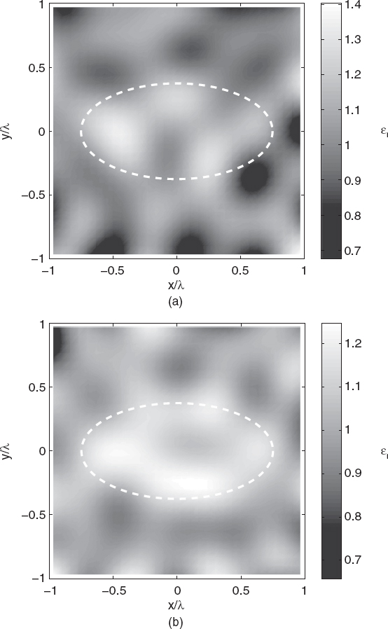
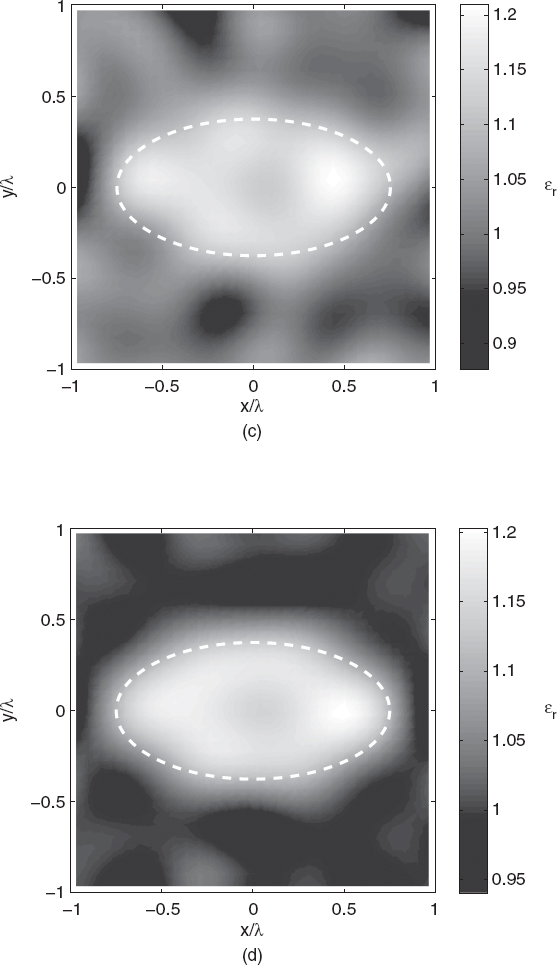
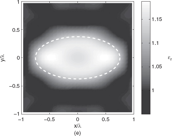
FIGURE 5.4 Reconstruction of the cross section of the homogenous lossless elliptic cylinder shown in Figure 5.1, First-order Born approximation and truncated SVD. Line-current illuminations (S = 8 sources, M = 55 measurement points on a circumference of radius 1.5λ). Square investigation domain (side: d = 2λ; discretization: 30 × 30 pixels). Complex dielectric permittivity: ε = (1.2 − j0;)ε₀. Gaussian noise: (a) SNR = 5dB; (b) SNR = 10dB; (c) SNR = 15dB; (d) SNR = 25dB; (e) SNR = 50dB. The dashed line in each plot indicates the original profile. (Simulations performed by A. Randazzo, University of Genoa, Italy.)

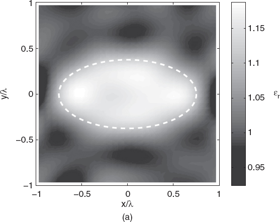
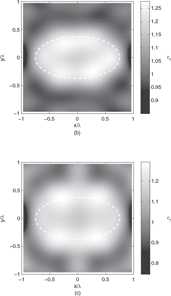
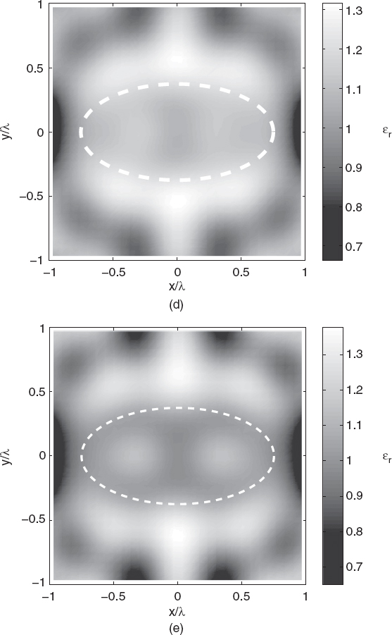
FIGURE 5.5 Reconstruction of the cross section of the homogenous lossless elliptic cylinder shown in Figure 5.1. The reconstruction method and the imaging configuration are the same as in Figure 5.4. Relative dielectric permittivity: (a) ε′_r = 1.2; (b) ε′_r = 1.4; (c) ε′_r = 1.6; (d) ε′_r = 1.8; (e) ε′_r = 2.0. The dashed line in each plot indicates the original profile. (Simulations performed by A. Randazzo, University of Genoa, Italy.)

Finally, the singular values related to the matrix decomposition are provided in Figure 5.6. It should be noted that a very similar formulation can be derived if the Rytov approximation described in Section 4.8 is applied. The computation is not repeated here.

TABLE 5.2 Relative Errors on Reconstruction of Elliptic Cylinders in Figure 5.4 for Different SNR Values, Calculated by First-Order Born Approximation Using the Truncated SVD Method

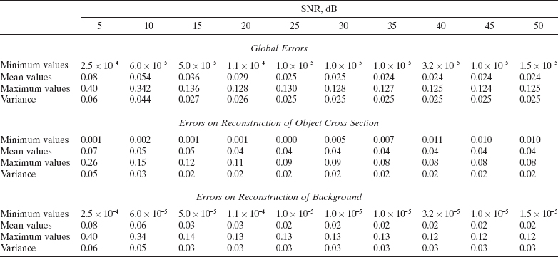
TABLE 5.3 Relative Errors on Reconstruction of Elliptic Cylinders in Figure 5.5 for Different Relative Dielectric Permittivity Values, Calculated by First-Order Born Approximation Using the Truncated SVD Method

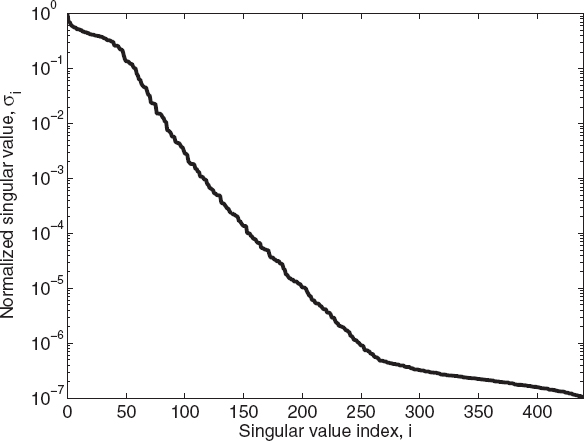
FIGURE 5.6 Singular values of the matrix used to obtain the reconstructions in Figure 5.5. (Simulations performed by A. Randazzo, University of Genoa, Italy.)

5.13 THE BORN ITERATIVE METHOD

The Born approximation discussed in Section 4.6 is also applied to develop iterative methods. The first method to be mentioned is the so-called Born iterative method, in which the initial object function is iteratively updated until a stopping criterion is satisfied. At each iteration the first-order Born approximation is applied.

With reference to equation (5.12.1), let us consider τ⁰ as a known initial guess distribution. If no a priori information is available, we can assume τ⁰(r) = 0 (the object coincides with the background). After the initialization step (k = 0) the approach iteratively evolves. At the kth step (k ≥ 1), the equations to be solved are as follows:

Equations (5.13.1) and (5.13.2) are not used together. In particular, at the kth iteration, the electric field inside the investigation domain S_i is first obtained by solving the state equation (5.13.1), where τ^k−1 is a known quantity. Afterward, the scattering potential τ^k is determined by using the data equation (5.13.2). In this equation the left-hand side is the known term of the problem (it is obtained from measurements performed in the observation domain S_m), and hence it does not depend on the iteration number k. The iterative approach finishes when a stopping criterion is satisfied.

It should be noted that the whole computation involves the solution of only linear integral equations, which can be numerically performed as mentioned in Section 3.4. It should also be noted that the same Green function is used at any iteration. This Green function is related to the background medium.

A variational form of this procedure has also been proposed in which the unknown distribution to be retrieved is not directly the object function, but the difference between the object functions at two different iterations (Zaiping et al. 2000).

5.14 RECONSTRUCTION OF EQUIVALENT CURRENT DENSITY

Besides inverse scattering problems, inverse source problems can be considered in microwave imaging. Such problems are aimed at reconstructing the equivalent current density, J_eq, and, as indicated by equation (3.2.3), they are linear. The issue is the information content of J_eq. It has been shown that some methods are based on the reconstruction of J_eq, including diffraction tomography (Section 5.11). However, in those cases, one needs some a priori information on the object, as in cases in which the Born approximation can be used (i.e., since the incident field is known, from J_eq one can immediately deduce the dielectric parameters of the unknown target, in particular, for dielectrics, the object function τ [equations (2.6.10) and (2.7.3)]. In the general case, the situation is different. In fact, the equivalent current density can be written as the sum of radiating and nonradiating components, that is

where the nonradiating source is such that the field that it produces is everywhere equal to zero except inside its support (Devaney and Wolf 1973). Since J_NR does not radiate outside V_o, it cannot be reconstructed starting from measurements performed outside V_o (i.e., in the observation domain). On the contrary, J_NR contributes to the field inside V_o. Consequently, the total field inside V_o can be written as

where

and

Consequently, if only the radiating component of J_eq is available, the term cannot, in general, be computed. Accordingly, the dielectric properties of the object to be inspected cannot be deduced from equation (2.6.10).

Moreover, the information on J_eq can be important when a priori information on the object is available, as in the case in which the Born approximation can be used. It has also been observed that nonradiating sources contribute to the higher spatial frequencies of the object to be inspected. Accordingly, neglecting them can result in a smoothing effect on the reconstruction, which can be acceptable in certain cases.

However, a possible approach that factors in both components of the equivalent current density is to first reconstruct its visible part with a standard method [applied to the solution of equation (5.14.3)] and, successively, retrieving the invisible part by enforcing the constraint that the unknown total electric field Eⁱ produced by the ith source and the unknown object function τ be consistent, (for any i) with the known incident field, by means of an optimization approach similar to that described in Section 6.7. These points are discussed further in the literature (Gamliel et al. 1989, Wallacher and Louis 2006, Caorsi and Gragnani 1999).

Alternatively, by considering a multiillumination approach (see Section 4.2), one obtains

We can observe that τ is independent of i, and, unlike trying to reconstruct both τ and Eⁱ, Eⁱ can be viewed as “an unwanted factor or multiplicative noise term which contains a certain range of spatial frequencies determined by the distribution of energy of the radiation field and its effective wavelength within the object” (Morris et al. 1995).

REFERENCES

Alexandrov, O. and F. Santosa, “A topology preserving level set method for shape optimization,” J. Comput. Phys. 204, 121–130 (2005).

Berg, J. M. and K. Holmström, “On parameter estimation using level sets,” SIAM J. Control Optim. 37, 1372–1393 (1999).

Bertero, M. and P. Boccacci, Introduction to Inverse Problems in Imaging, Institute of Physics, Bristol, UK, 1998.

Bertero, M., M. Miyakawa, P. Boccacci, F. Conte, K. Orikasa, and M. Furutani, “Image restoration in chirp pulse microwave CT (CP-MCT),” IEEE Trans. Biomed. Eng. 47, 690–699 (2000).

Bolomey, J.-C., A. Izadnegahdar, L. Jofre, Ch. Pichot, G. Peronnet, and M. Solaimani, “Microwave diffraction tomography for biomedical applications,” IEEE Trans. Microwave Theory Tech. 30, 1998–2000 (1982).

Bond, E. J., X. Li, S. C. Hagness, and B. D. Van Veen, “Microwave imaging via space-time beamforming for early detection of breast cancer,” IEEE Trans. Anten. Propag. 51, 1690–1705 (2003).

Burger, M., “A level set method for inverse problems,” Inverse Problems 17, 1327–1355 (2001).

Burger, M. and S. Osher, “A survey on level set methods for inverse problems and optimal design,” Eur. J. Appl. Math. 16, 263–301 (2005).

Cakoni, F. and D. Colton, Qualitative Methods in Inverse Scattering Theory, Springer, Berlin, 2006.

Caorsi, S., S. Ciaramella, G. L. Gragnani, and M. Pastorino, “On the use of regularization techniques in numerical inverse-scattering solutions for microwave imaging applications,” IEEE Trans. Microwave Theory Tech. 43, 632–640 (1995).

Caorsi, S. and G. L. Gragnani, “Inverse-scattering method for dielectric objects based on the reconstruction of the nonmeasurable equivalent current density,” Radio Sci. 34, 1–8 (1999).

Caorsi, S., M. Pastorino, and M. Raffetto, “Electromagnetic scattering by a multilayer elliptic cylinder under line-source illumination,” Microwave Opt. Technol. Lett. 24, 322–329 (2000).

Catapano, I., L. Crocco, and T. Isernia, “On simple methods for shape reconstruction of unknown scatterers,” IEEE Anten. Propag. 55, 1431–1435 (2007).

Chen, Y., E. Gunawan, K. S. Low, S. C. Wang, C. B. Soh, and L. L. Thi, “Time of arrival data fusion method for two-dimensional ultra wideband breast cancer detection,” IEEE Trans. Anten. Propag. 55, 2852–2865 (2007).

Colton, D., H. Haddar, and M. Piana, “The linear sampling method in inverse electromagnetic scattering theory,” Inverse Problems 19, S105–S137 (2003).

Colton, D. and R. Kress, Inverse Acoustic and Electromagnetic Scattering Theory, Springer, Berlin, 1998.

Colton, D. and P. Monk, “A linear sampling method for the detection of leukemia using microwaves,” SIAM J. Appl. Math. 58, 926–941 (1998).

Datta, A. N. and B. Bandyopadhyay, “An improved SIRT-style reconstruction algorithm for microwave tomography,” IEEE Trans. Biomed. Eng. 32, 719–723 (1985).

Devaney, A. J., “A computer simulation study of diffraction tomography,” IEEE Trans. Biomed. Eng. 30, 377–386 (1983).

Devaney, A. J., “Reconstructive tomography with diffracting wavefields,” Inverse Problems 2, 161–183 (1986).

Devaney, A. J. and E. Wolf, “Radiating and nonradiating classical current distributions and the fields they generate,” Phys. Rev. D 8, 1044–1047 (1973).

Dorn, O. and D. Lesselier, “Level set methods for inverse scattering,” Inverse Problems 22, R67–R131 (2006).

Dorn, O., E. Miller, and C. Rappaport, “A shape reconstruction method for electromagnetic tomography using adjoint fields and level sets,” Inverse Problems 16, 1119–1156 (2000).

Ferraye, R., J. Y. Dauvignac, and C. Pichot, “An inverse scattering method based on contour deformations by means of a level set method using frequency hopping technique,” IEEE Trans. Anten. Propag. 51, 1100–1113 (2003).

Franchois, A., A. Joisel, C. Pichot, and J.-C. Bolomey, “Quantitative microwave imaging with a 2.45-GHz planar microwave camera,” IEEE Trans. Med. Imag. 17, 550–561 (1998).

Gamliel, A., K. Kim, A. I. Nachman, and E. Wolf, “A new method for specifying nonradiating monochromatic scalar sources and their fields,” J. Opt. Soc. Am. 6, 1388–1393 (1989).

Hajihashemii, M. R. and M. El-Shenawee, “Shape reconstruction using the level-set method for microwave applications,” IEEE Anten. Wireless Propag. Lett. 7, 92–96 (2008).

Kak, A. C. and M. Slaney, Principles of Computerized Tomographic Imaging. IEEE Press, New York, 1988.

Li, X., E. J. Bond, B. D. Van Veen, and S. C. Hagness, “An overview of ultra-wideband microwave imaging via space-time beamforming for early-stage breast-cancer detection,” IEEE Anten. Propag. Mag. 47, 19–29 (2005).

Litman, A., “Reconstruction by level sets of n-ary scattering obstacles,” Inverse Problems 21, S131–S152 (2005).

Litman, A., D. Lesselier, and D. Santosa, “Reconstruction of a two-dimensional binary obstacle by controlled evolution of a level-set,” Inverse Problems 14, 685–706 (1998).

Maini, R., M. F. Iskander, C. H. Durney, and M. Berggren, “On the sensitivity and the recolution of microwave imaging using ART,” Proc. IEEE 69, 1517–1519 (1981).

Mohan, A. S. and F. Yang, “Improved beamforming for microwave imaging to detect breast cancer,” Proc. 2009 Antennas Propagation Society Int. Symp. 2009.

Morris, J. B., F. C. Lin, D. A. Pommet, R. V. McGahan, and M. A. Fiddy, “A homomorphic filtering method for imaging strongly scattering penetrable objects,” IEEE Anten. Propag. 43, 1029–1035 (1995).

Oden, T. J. and L. F. Demkowicz, Applied Functional Analysis, CRC Press, Boca Raton, FL, 1996.

Pichot, C., L. Jofre, G. Peronnet, and J.-C. Bolomey, “Active microwave imaging of inhomogeneous bodies,” IEEE Trans. Anten. Propag. 33, 416–425 (1985).

Pike, E. R. and P. C. Sabatier, eds., Scattering and Inverse Scattering in Pure and Applied Science, Academic Press, London, 2001.

Ramananjaona, C., M. Lambert, D. Lesselier, and J. P. Zolesio, “Shape reconstruction of buried obstacles by controlled evolution of a level set: From a min-max formulation to numerical experimentation,” Inverse Problems 17, 1087–1111 (2001).

Rudin, W., Real and Complex Analysis, McGraw-Hill, New York, 1970.

Sarkar, T., D. Weiner, and V. Jain, “Some mathematical considerations in dealing with the inverse problem,” IEEE Trans. Anten. Propag. 29, 373–379 (1981).

Tikhonov, A. N., A. V. Goncharsky, V. V. Stepanov, and A. G. Yagola, Numerical Methods for the Solution of Ill-Posed Problems, Springer, Berlin, 1995.

Tsihrintzis, G. A. and A. J. Devaney, “Higher order (nonlinear) diffraction tomography: Inversion of the Rytov series,” IEEE Trans. Inform. Theory 46, 1748–1761 (2000).

Wallacher, E. and A. K. Louis, “Complete set of radiating and nonradiating parts of a source and their fields with applications in inverse scattering limited-angle problems,” Int. J. Biomed. Imag. 2006, 1–13 (2006).

Zaiping, N., Y. Feng, Z. Yanwen, and Z. Yerong, “Variational Born iteration method and its applications to hybrid inversion,” IEEE Trans. Geosci. Remote Sens. 38, 1709–1715 (2000).