CHAPTER FOUR

Imaging Configurations and Model Approximations

4.1 OBJECTIVES OF THE RECONSTRUCTION

In practical applications, the objectives of the inspection can be very different. In certain cases, it can be sufficient to locate the unknown scatterers by retrieving their spatial positions starting from measurement of the scattered field performed outside an investigation domain. Methods aimed at solving this problem are actually not imaging methods, but mainly localization methods (e.g., those based on radar concepts and on smart antennas that can estimate the directions of arrival of signals related to the presence of the objects).

In other cases, the aim of the inspection is to retrieve the shape of the object, which in certain applications (discussed in the following sections) is sufficient information, as the values of the object's dielectric parameters are unnecessary or obvious. An example is represented by nondestructive testing, evaluations, and quality control of materials and products (see Chapter 10), where knowledge of the position and shape of a defect is often sufficient for deciding whether the structure of apparatus under test can be still used. Moreover, the information on the shape and, consequently, on the dimensions of a defect can also be an indication for determining the residual life of the apparatus or system.

However, the most ambitious goal of the inspection is to obtain complete images of the objects under test. Such images, when using microwaves, are directly related to the spatial distributions of the dielectric parameters of the scattering targets.

In the following sections, the most common configurations used in microwave imaging systems are presented, with particular focus on the assumption made regarding measurement points and illumination conditions. Tomographic configurations are presented in detail for their significant practical relevance. However, scanning configurations are also considered. The chapter also describes the most frequently used approximations for simplyfing, when possible, the scattering equations. Finally, the problem of numerical computation of Green's function for arbitrary inhomogeneous background is discussed.

4.2 MULTIILLUMINATION APPROACHES

In general, the object to be inspected is sequentially illuminated by using a set of incident fields that are generated by several transmitting antennas or by a single source moving around the target. For each illuminating field, the measurements are performed in an observation domain that can be the same for each incident field or can change at any illumination. If the investigation domain V_i remains unchanged during the measurement phase, the following set of integral equations [see (3.2.1) and (3.2.2)] is obtained:

Here, the superscript i denotes quantities related to the ith illumination (except, of course, in the symbol for the investigation domain V_i) and indicates the observation domain where the samples of the field are collected when the ith incident field is applied. On the other hand, if the observation domain does not change during the measurement phase, then = V_m for any i. By considering equations (4.2.1) and (4.2.2), one can observe that the object function does not depend on i, whereas the total internal field changes for any illumination.

Analogous relations hold if the contrast source formulation is adopted [see (3.2.3) and (3.2.4) ]

where the contrast sources are dependent on the considered incident field.

4.3 TOMOGRAPHIC CONFIGURATIONS

A classical example of the multiillumination process is represented by microwave tomography, which is used for two-dimensional imaging (Kak and Slaney 1988). With reference to Figure 4.1, in tomographic applications, the observation domain is usually a circle including the cross section of the target to be inspected or a rotating straight line always tangent to a circle surrounding the target. Under transverse magnetic (TM) illumination conditions, the two-dimensional counterparts of equations (4.2.1) and (4.2.2) are

where indicates the observation domain where the measured values related to the ith illumination are collected. Analogous relationships hold if the contrast source formulation is used:

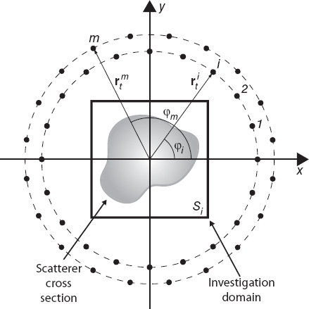
FIGURE 4.1 Two-dimensional imaging configuration, showing object cross section and investigation area and positions of the sources and measurement points.

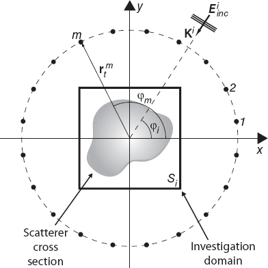
FIGURE 4.2 Two-dimensional imaging configuration; plane-wave illumination.

The target is successively illuminated by S incident fields incoming from different directions. If plane-wave illumination can be assumed (Fig. 4.2), then, according to equation (2.4.24), the incident field is given by

where kⁱ = . If the incident waves are equally angularly spaced, the incident angle φ_inc assumes the following values:

In other cases, as mentioned in Section 2.4, the illuminating field is modeled as the one produced by a line-current source (Fig. 4.3). In that case, taking into account equation (2.4.26), we obtain

where , with Iⁱ and such that . Obviously, in the plane z = 0, the ith line-current source passes through point . If the sources are located on a circumference or radius ρ_s (with polar coordinates), then . Moreover, if points , i = 1,..., S, are equally spaced on this circle, φ_i is again as given by equation (4.3.6).

It should be noted that the source can be modeled more realistically by factoring in the radiation pattern of the transmitting antenna. However, in most cases, the radiation pattern is sufficiently wide (in the azimuth plane z = 0) to illuminate the entire investigation domain, so that the above models for the incident field are usually adopted.

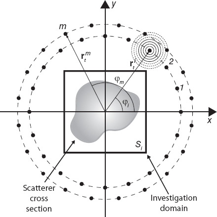
FIGURE 4.3 Two-dimensional imaging configuration; line-current sources.

A simple method for shaping the incident field to better approximate the radiation properties of the transmitting antenna is to use a relation similar to Silver's formula (Balanis 2005), which is valid for the main lobe of the antenna. In this case (Fig. 4.4), for an antenna located at and radiating toward the center of the coordinate system (which coincides with the center of the investigation domain), the following relation holds

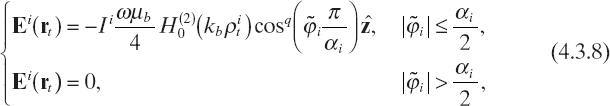
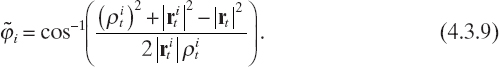
where α_i is the beamwidth of the main lobe of the ith antenna in the z = 0 plane and is the azimuth angle in the local coordinate system of the ith antenna, which can be expressed as follows:

In equation (4.3.8), q is an exponent controlling the directivity of the antenna; the more directive is the antenna, the higher is q. For isotropic (in the transverse plane) antennas, the result is q = 0.

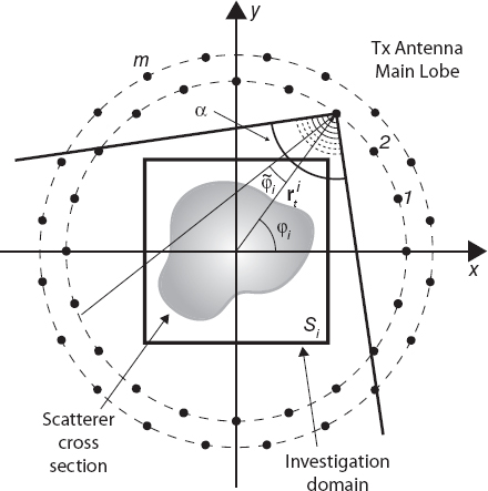
FIGURE 4.4 Two-dimensional imaging configuration; main lobe of the transmitting antenna.

As mentioned in Section 3.4, the measurements are usually performed in a discrete set of points. These measurement points can completely surround the object cross section; that is, they can be located on a circumference of radius ρ_M. This circumference may (ρ_M = ρ_S) or may not (ρ_M ≠ ρ_S) coincide with the one in which the sources are located. In this case, the measurement points (assumed to be the same for any illumination) are located at , m = 1,..., M, where

Sometimes, one tries to avoid placing measurement points near the sources. This can be achieved by locating the probes, for the ith illumination, at points , m = 1,..., M, i = 1,..., S, such that

where β is an angular sector around the incident direction φ_i, where no measurement points are present.

In other cases, the measurement points can be located on a straight line on the opposite side of the object from the source of the incident field (Fig. 4.5). This measurement line (probing line) should ideally be infinite in order to measure the entire scattered wave. In real applications, the probing line should be long enough to capture most of the energy of the scattered wave. In this case, a set of M measurement points of coordinates , m = 1,..., M, i = 1,..., S, such that

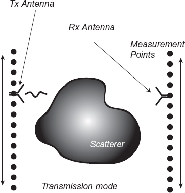
FIGURE 4.5 Two-dimensional imaging configuration for data acquisition in transmission mode; linear probing line.

where , i = 1,..., S is the center of the linear probing line for the ith view and κⁱ is the related angular coefficient.

4.4 SCANNING CONFIGURATIONS

With reference to Figure 4.6, the inspection can be performed on a single side of the object. In this case, the reflection is the main measured contribution to the input data. A set of measurement M points, , m = 1,..., M, are usually located on a straight line (although other configurations are possible), for which equation (4.3.12) still holds. A single probe can be used (Fig. 4.6), which is moved to occupy successively the various positions . In this case, the probe location coincides with a given measurement point. At each position of the probe, the scattered field is measured (monostatic configuration). An image of the target based only on the measured scattered field can be constructed.

Otherwise, the measured values can be stored and postprocessed in order to combine the reflected signals to obtain a synthetic aperture focusing (see Chapter 5).

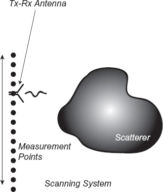
FIGURE 4.6 Two-dimensional imaging configuration for data acquisition in reflection mode; scanning systems, with single probe and linear probing line.

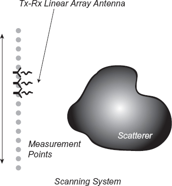
FIGURE 4.7 Two-dimensional imaging configuration for data acquisition in reflection mode; scanning systems, with linear array probe.

An array of probes can also be used (Fig. 4.7). Consequently, for each position of the transmitting element , the field scattered can be collected in a set of points , m = 1,..., Q, in which Q can coincide with M or can be a subset of the scanned domain (Q ≤ M).

4.5 CONFIGURATIONS FOR BURIED-OBJECT DETECTION

To detect a shallow buried object, the source and the probes are usually located in the upper region (Fig. 4.8). In this case, the measurement points are , where y₀ is the distance of the probing line from the interface between air and the medium in which the target is located (e.g., the soil), assumed to be the line y = 0. Accordingly, in equation (4.3.12), κⁱ = 0. Moreover, the same scanning approaches discussed in Section 4.4 can be adopted.

When possible, a borehole configuration can be used. With reference to Figure 4.9, the source(s) and the probe(s) can be located inside holes. Actually, this technique is used mainly at lower frequencies and usually results in better reconstructions, due to the possibility of accounting for more contributions to the scattering mechanism. In the borehole configuration, the points in which the sources are positioned are denoted as , s = 1,..., S, with y^s < 0 and x₁ denoting the x coordinate of the center of the source hole, whereas the measurement points are , m = 1,..., M, y^m < 0, where x₂ is the x coordinate of the center of the measurement hole.

4.6 BORN-TYPE APPROXIMATIONS

In some cases, information on the target under test are available. Consequently, approximations of the model can be introduced. When the scatterer to be inspected is weak with respect to the propagation medium, Born-type approximations can be used (Morse and Feshbach 1953, Born and Wolf 1965). The simplest approximation is the first-order Born approximation, which assumes that the scattered electric field in equation (2.7.2) can be written only in terms of the incident field:

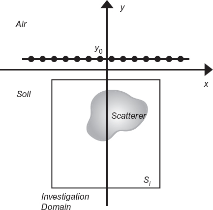
FIGURE 4.8 Two-dimensional imaging configuration for buried-object detection.

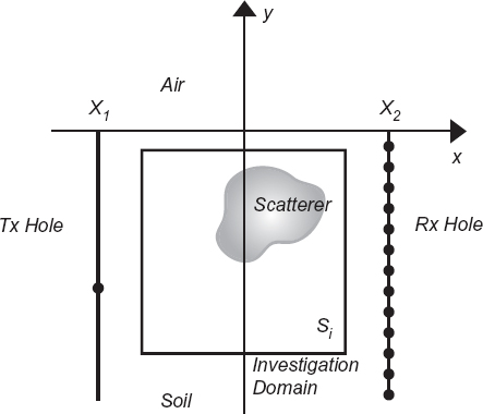
FIGURE 4.9 Two-dimensional configuration for bore-hole imaging of buried objects.

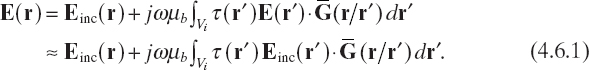
Accordingly, we shall write

where the superscript 1B indicates the approximation presented above.

The Born approximation can be used for both the direct scattering problem (i.e., to compute the field scattered by a known weakly scattering object) and the inverse scattering problem (i.e., to reconstruct an unknown target). In particular, in the inverse scattering problem under the approximation given above, the scattering equation (2.7.2) is linearized, since the only problem unknown is the object function τ(r), r ∈ V_i, where V_i is the investigation domain defined in Section 3.2. More precisely, the first-order Born approximation is valid for weak scatterers for which (Natterer 2004)

where a is the radius of the minimum circle that can include the object cross section and ς is a constant that Slaney et al. (1984) set to 0.25, even if different estimations have been proposed (Natterer 2004, Chen and Stamnes 1998). The choice ς = 0.25 is obtained in the Slaney et al. (1984) study by considering a plane wave impinging onto a cylindrical scatterer and requiring that the phase change between the incident wave and the field traveling through the scatterer be less than π.

Higher-order Born approximations can be obtained in a recursive way. In particular, a Born series can be constructed by using the following recursive relations

where the superscript nB denotes the nth-order approximation. Although this series can be used for a fast solution of the direct scattering problem, it converges only for weak scatterers. Moreover, in microwave imaging, besides the first-order approximation, the second-order approximation has been considered in some studies (Pierri et al. 2000, Estatico et al. 2005). In this case (n = 2), and according to (4.6.4), we have

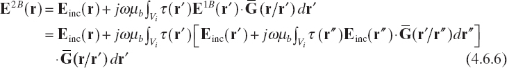
which is a quadratic equation with respect to the object function. Moreover, it seems that it can limitedly extend, in practice, the range of applicability of the first-order approximation. The key point in applying this approximation is that the resulting inverse problem is still nonlinear, but only the object function is unknown. This represents a significant savings in computation in comparison to the approaches for which the total electric field inside the target is kept as an additional unknown.

As has been shown (Estatico et al. 2005), the second-order Born approximation provides better reconstructions when the Born series converges [essentially, under condition (4.6.3)].

In two-dimensional problems (see Section 3.3), equation (4.6.2) becomes

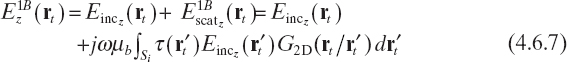
where E_incz (r_t) and turn out to be the solutions of the scalar Helmholtz equations

where J_z and are z components of the impressed source [equation (2.3.13)] and of the equivalent current density [equation (3.3.15)] written under the first-order Born approximation:

Obviously, equations (4.6.8) and (4.6.9) can be deduced with some trivial mathematical steps from the corresponding vector wave equations (in the form of equation (2.4.1)) by using the transverse-magnetic assumptions stated in Section 3.3 (Chew 1990).

4.7 EXTENDED BORN APPROXIMATION

Let us consider a point r ∈ V_o located inside the object. By factoring in the definition of the equivalent source in terms of scattering potential, we can rewrite equation (2.7.1) as

If the quantity is added and subtracted from equation (4.7.1), we obtain (Habashy et al. 1993)

or, equivalently

If one now considers the fact that Green's function is highly peaked when r → r′ (due to its singularity) and, on the contrary, tends to zero when |r – r′| → ∞, the following approximate relation can be obtained:

As a consequence, we have

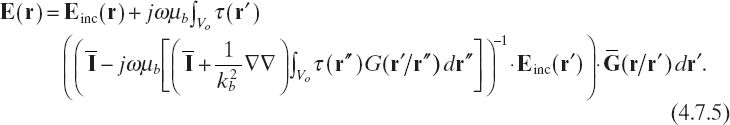
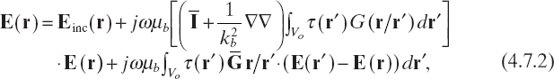
Equation (4.7.5) is a nonlinear integral equation in the only unknown τ, which can be shown to extend the range of validity of the first-order Born approximation (Habashy et al. 1993). The approximation adopted to derive such a scattering equation is referred to as the extended Born approximation, which can be also used in two-dimensional scattering problem with TM illumination (see Section 3.3). To this end, let us consider equation (3.3.8), for r_t ∈ S_o. An equivalent integral equation can be derived from that equation if the quantity is added and subtracted on the right-hand side:

By rearranging terms, we obtain

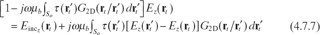
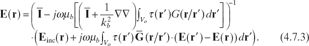
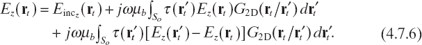
As a consequence, the internal electric field can be expressed as

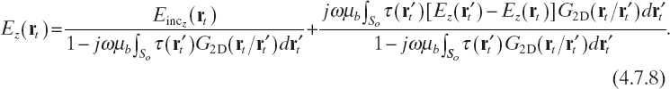
It is worth noting that no approximation has been introduced so far. However, since Green's function in this case is also a highly peaked function when r_t → r′_t, because of its singularity but tends to zero for |r_t – r′_t| → ∞, the second term on the right-hand side can be neglected and the extended Born approximation is obtained for the internal field in two-dimensional TM scattering as follows:

The corresponding integral equation describing the scattering phenomena then reads as

As already observed for three-dimensional configurations, the equation obtained is still nonlinear, but involves as unknown only the scattering potential. Moreover, the range of validity of such an approximation has been shown to be wider than the classical Born one (Zhang and Liu 2001, Habashy et al. 1994, Song and Liu 2005, Torres-Verdin and Habashy 2001).

For the sake of completeness, it is worth remarking that the extended Born approximation presented above can be generalized and extended to higher-order approximations, as described in by Gao and Torres-Verdin (2006) and in Cui et al. (2004).

4.8 RYTOV APPROXIMATION

The Rytov approximation is another first-order approximation, which is based on the phase of the electromagnetic field. In this section, for simplicity, only the scattering by two-dimensional configurations under TM illumination conditions is considered.

The first step for applying the Rytov approximation, consists in expressing the incident field as (Slaney et al. 1984)

where Φ_inc(r_t) is the incident complex phase function. Analogously, the total field is written as

where Φ(r_t) is the total complex phase function. By using Φ_inc(r_t) and Φ(r_t), one can define the scattered phase:

Since

and

we obtain

Moreover, because

holds for a scalar field and a vector field, ψ and F, respectively, it follows that

Let us now consider the scalar Helmholtz equation for the scattered field produced by the equivalent current density

which is analogous to equation (4.6.9) with the exact equivalent current density J_eqz (r_t) instead of (r_t). Since the incident field satisfies the Helmholtz equation (4.6.8), for points inside the investigation domain (i.e., r_t ∈ S_i), where the impressed source is equal to zero, from (4.8.9) and (4.6.8) it follows that

By substituting (4.8.8) into (4.8.10), and taking into account (4.8.2) we obtain the following Riccati equation

and, using (4.8.3), we have

With similar mathematical steps, starting from the equation for the incident field [equation (4.6.8), which is a homogeneous equation for r_t ∈ S_i], we obtain

Using (4.8.12) and (4.8.13), we then obtain

Moreover, from the following identity

we deduce that

In deriving equation (4.8.16), we have accounted for

and

Finally, comparing (4.8.16) with (4.8.14), we obtain

The Rytov approximation requires that the variations of the complex scattered phase be neglected for r_t ∈ S_i (Ishimaru 1978). Accordingly, the solution of equation (4.8.19) can be written in terms of Green's function for two-dimensional configurations as

which is a linear integral equation having as unknown term only the object function τ, which includes the dielectric properties of the cross sections of the scatterers inside the investigation area S_i [equation (2.7.3)].

It has been argued that the Rytov approximation, as compared with the first-order Born approximation (Section 4.6), is better for larger objects with small changes in the dielectric permittivity distribution (Slaney et al. 1984). However, for small scatterers, the two approximations tend to coincide, in fact, from equation (4.8.3) we have

If the amplitude of the scattered field inside the scatterer is very small, the second term in square brackets can be neglected and E_z(r_t) ≈ E_incz (r_t) results. The Rytov approximation simplifies to the Born approximation.

However, it has been shown that a condition for the validity of the Rytov approximation is (Slaney et al. 1984, Keller 1969)

It has also been observed that “unlike the Born approximation, the size of the object is not a factor in the Rytov approximation” (Slaney et al. 1984). Since the approximation concerns phase changes, the Rytov approximation is expected to work well with smoothly varying dielectric profiles for which the phase change is small (Dunlop et al. 1976).

4.9 KIRCHHOFF APPROXIMATION

In the inspection of PEC scatterers, at high frequencies, use of the Kirchhoff approximation (or physical optics (PO) approximation) has been proposed even for short-range imaging (Pierri et al. 2001). With reference to equation (2.8.1), the unknown current density on the surface S is approximated as

where S₁ and S₂ are the illuminated and shadowed parts of S, with S = S₁ ∪ S₂. Clearly, the only problem unknown is now the support of the scatterer, in particular the surface S₁.

It should be noted that imaging methods developed in the high-frequency range (i.e., methods for inspecting objects whose linear dimensions are much higher than the wavelength of the incident field) are not considered in the present book. These techniques are usually based on geometric optics approximations and ray propagation. The reader is referred to the article by Chu and Farhat (1988) and the references therein.

4.10 GREEN'S FUNCTION FOR INHOMOGENEOUS STRUCTURES

So far it has been assumed that the object to be inspected is immersed in free space (Figs. 4.1–4.7) or in a half-space domain (Figs. 4.8 and 4.9). In both cases, the Green functions/tensors involved in the computation are known quantities given by relations (2.4.7), (3.3.9), (2.4.12), and (2.4.13). In some imaging applications, however, the object can be immersed in an inhomogeneous medium, for which a closed-form relation for Green's function is seldom available.

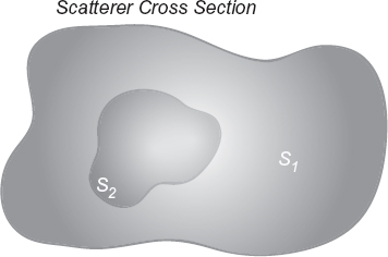
FIGURE 4.10 Cross section of an infinite cylinder with two separated regions.

However, this Green function can be computed numerically. There are two motivations for studying the inhomogeneous Green function for a given structure. The first one concerns the practical case in which the object to be detected is a defect inside an otherwise known target. If the Green's function for the propagation medium constituted by the unperturbed target is known, the inspection can be limited to a reduced investigation domain inside the target, avoiding the need for inspecting the whole body. The second reason for studying the inhomogeneous Green's function is related to development of the distorted Born iterative method, discussed in Section 6.6.

With reference to two-dimensional scattering, let us consider Figure 4.10, in which an object of support S₁ includes a region of interest S₂ ⊂ S₁. In some cases, the two domains can coincide. Given an incident field, the total field inside and outside the object can be computed by using equation (3.3.8). Alternatively, we can express the complex dielectric permittivity of the inner part of the object S₁ in this way

where ε₁(r_t) = ε(r_t) for r_t ∈ S₁ and ε₂(r_t) = ε(r_t) for r_t ∈ S₂. For example, region S₂ can be a defect in an otherwise known object. In this case ε₁(r_t) is known for any r_t ∈ S₁. In other cases, the values of ε₁(r_t) for r_t ∈ S₂ could be fixed arbitrarily (it is also not a theoretical requirement that S₂ ⊂ S₁ although this is a situation that can be encountered in practical imaging problems).

According to equation (4.10.1), the object function of equation (3.3.8) can be rewritten as

where

and

By considering (4.10.3) and (4.10.3), from equation (3.3.8) we obtain

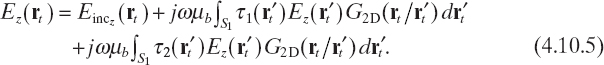
Alternatively (Fig. 4.10), the field E_z can be viewed as the sum of the field scattered by the excess of permittivity of region S₂ when the incident field is the field that propagates in an inhomogeneous medium that is characterized by ε_b for r_t ∉ S₁ and by ε₁(r_t) for r_t ∈ S₁, specifically,

where E_1z is given by

and G_in is Green's function for the inhomogeneous structure S₁. By definition (Tai 1971), it satisfies equation

Let us consider again the case in which one searches for a defect in a known structure. Green's function for this structure can be computed offline and stored. Then, an imaging method (e.g., one of those described in the following chapters) can be applied with reference to a reduced investigation domain coinciding with S₂. This essentially allows the imaging system to focus on a certain region of the original configuration.

Moreover, even in the case in which S₁ ≡ S₂, one can search for a small perturbation over a prescribed dielectric configuration. This is essentially the approach followed in the development of the distorted-wave Born approximation (Section 6.6), which is a very effective microwave imaging technique.

In order to numerically solve equation (4.10.6) according to the approach described in Section 3.4, it is necessary to calculate the following integrals [see equation (3.4.6)]

which can be approximated by

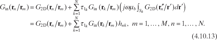
where r_n is the center of the nth subdomain. To calculate the values of G_in(r_m/r_n), used in (4.10.10), the following set of integral equations must be solved [see (4.10.8)]:

By exploiting the reciprocity of Green's function, we have

and by following a procedure similar to that reported in Section 3.4, we obtain

The set of equations in (4.10.13) can also be expressed in matrix form as

where [G] is a rectangular N × M matrix, whose elements are the values of the inhomogeneous Green function G_in(r_n/r_m), [G_2D] is a rectangular N × M matrix, whose elements are the values of the free-space Green function G_2D(rn/rm), and [T₁] is a square N × N diagonal matrix whose diagonal elements are given by τ_1n, n = 1,..., N.

Consequently, computation of the inhomogeneous Green function is reduced to resolution of the matrix equation given by (4.10.14), whose solution is

where [I] is the N × N identity matrix.

REFERENCES

Balanis, C. A., Antenna Theory: Analysis and Design, Wiley, Hoboken, NJ, 2005.

Born, M. and E. Wolf, Principles of Optics, Pergamon Press, New York, 1965.

Chen, B. and J. J. Stamnes, “Validity of diffraction tomography based on the first Born and the first Rytov approximations,” Appl. Opt. 37, 2996–3006 (1998).

Chew, W. C., Waves and Fields in Inhomogeneous Media, Van Nostrand Reinhold, New York, 1990.

Chu, T. H. and N. H. Farhat, “Frequency-swept microwave imaging of dielectric objects,” IEEE Trans. Microwave Theory Tech. 36, 489–493 (1988).

Cui, T. J., Y. Qin, G.-L. Wang, and W. C. Chew, “Low-frequency detection of two-dimensional buried objects using high-order extended Born approximations,” Inverse Problems 20, 41–62 (2004).

Dunlop, G., W. Boerner, and R. Bates, “On an extended Rytov approximation and its comparison with the Born approximation,” Proc. Antennas Propagation Society Int. Symp. 1976, pp. 587–591.

Estatico, C., M. Pastorino, and A. Randazzo, “An inexact Newton method for short-range microwave imaging within the second order Born approximation,” IEEE Trans. Geosci. Remote Sens. 43, 2593–2605 (2005).

Gao, G. and C. Torres-Verdin, “High-order generalized extended Born approximation for electromagnetic scattering,” IEEE Trans. Anten. Propag. 54, 1243–1256 (2006).

Habashy, T. M., R. W. Groom, and B. R. Spies, “Beyond the Born and Rytov approximations: A nonlinear approach to electromagnetic scattering,” J. Geophys. Res. 98, 1759–1775 (1993).

Habashy, T. M., M. L. Oristaglio, and A. T. de Hoop, “Simultaneous nonlinear reconstruction of two-dimensional permittivity and conductivity,” Radio Sci. 29, 1101–1118 (1994).

Ishimaru, A., Wave Propagation and Scattering in Random Media, Academic Press, New York, 1978.

Kak, A. C. and M. Slaney, Principles of Computerized Tomographic Imaging, IEEE Press, New York, 1988.

Keller, J. B., “Accuracy and validity of the Born and Rytov approximations,” J. Opt. Soc. Am. 59, 1003–1004 (1969).

Morse, P. M. and M. Feshbach, Methods of Theoretical Physics, McGraw-Hill, New York, 1953.

Natterer, F., “An error bound for the Born approximation,” Inverse Problems 20, 447–452 (2004).

Pierri, R., G. Leone, and R. Persico, “Second-order iterative approach to inverse scattering: Numerical results,” J. Opt. Soc. Am. A 17, 874–880 (2000).

Pierri, R., A. Liseno, and F. Soldovieri, “Shape reconstruction from PO multifrequency scattered fields via the singular value decomposition approach,” IEEE Trans. Anten. Propag. 49, 1331–1343 (2001).

Slaney, M., A. C. Kak, and L. E. Larsen, “Limitations of imaging with first-order diffraction tomography,” IEEE Trans. Microwave Theory Tech. 32, 860–874 (1984).

Song, L.-P. and Q. H. Liu, “A new approximation to three-dimensional electromagnetic scattering,” IEEE Geosci. Remote Sens. Lett. 2, 238–242 (2005).

Tai, C. T., Dyadic Green's Functions in Electromagnetic Theory, Intext, Scranton, PA, 1971.

Torres-Verdin, C. and T. M. Habashy, “Rapid numerical simulation of axisymmetric single-well induction data using the extended Born approximation,” Radio Sci. 36, 1287–1306 (2001).

Zhang, Z. Q. and Q. H. Liu, “Two nonlinear inverse methods for electromagnetic induction measurements,” IEEE Trans. Geosci. Remote Sens. 39, 1331–1339 (2001).