
Chapter 2
Multivariate data modeling methods
The last chapter has introduced the principles of SPC and motivated the required multivariate extension to prevent excessive Type II errors if the recorded process variables are highly correlated. The aim of this chapter is to present different methods that generate a set of t-variables that are defined as score variables. Under the assumption that the process variables follow a multivariate Gaussian distribution, these score variables are statistically independent to circumvent increased levels of Type II errors. According to Figures 1.7 and 1.8, the generation of these score variables relies on projecting the recorded samples onto predefined directions in order to extract as much information from the recorded process variables as possible.
The data reduction techniques, introduced in the literature, are firmly based on the principle of establishing sets of latent variables that capture significant and important variation that is encapsulated within the recorded data. The score variables form part of these latent variable sets. For process monitoring, the variation that the latent variable sets extract from the recorded process variables is of fundamental importance for assessing product quality, process safety and, more generally, whether the process is in-statistical-control. These aspects are of ever growing importance to avert risks to the environment and to minimize pollution.
Data analysis and reduction techniques can be divided into single-block and dual-block techniques. The most notable single-block techniques include:
- Principal Component Analysis (Pearson 1901);
- Linear or Fisher's Discriminant Analysis (Duda and Hart 1973); and
- Independent Component Analysis (Hyvärinen et al. 2001).
Dual-block techniques, on the other hand, divide the recorded data sets into one block of predictor or cause variables and one block of response or effect variables and include:
- Canonical Correlation Analysis (Hotelling 1935; Hotelling 1936);
- Reduced Rank Regression (Anderson 1951);
- Partial Least Squares (Wold 1966a,b); and
- Maximum Redundancy (van den Wollenberg 1977),
among others. These listed single- and dual-block techniques are collectively referred as latent variable techniques.
From this list of techniques, the focus in the research literature has been placed on variance/covariance-based techniques as most appropriate for process monitoring applications. This has been argued on the basis of capturing the process variation, that is, encapsulated in the variance among and the covariance between the recorded process variables. These techniques are Principal Component Analysis (PCA) and Partial Least Squares (PLS), which are discussed and applied in this chapter and described and analyzed in Part IV of this book.
It should be noted that the research community has also developed latent variable techniques for multiple variable blocks, referred to as multi-block methods (MacGregor et al. 1994; Wangen and Kowalski 1989). These methods, however, can be reduced to single-block PCA or dual-block PLS models, for example discussed in Qin et al. (2001), Wang et al. (2003), Westerhuis et al. (1998). The methods used in this book are therefore limited to PCA and PLS.
As the focus for presenting MSPC technology in this chapter is based on its exploitation as a statistically based process monitoring tool, details of PCA and PLS are given using an introduction of the underlying data model, a geometric analysis and by presenting simple simulation examples in Sections 2.1 and 2.2, respectively. This allows a repetition of the results in order to gain familiarization with both techniques. A detailed statistical analysis of both techniques are given in Chapters 2 and Chapters 10.
Section 2.3 presents an extension of the PLS algorithm after analyzing that PCA and PLS fail to produce a latent variable data representation for a more general data structure. The validity of the general data structure is demonstrated by an application study of a distillation process in Part II of this book, which also includes an application study involving the applications of PCA. Section 2.4 then introduces methods for determining the number of the latent variable sets for each method. To enhance the learning outcomes, this chapter concludes with a tutorial session including short questions and calculations as well as homework type projects in Section 2.5.
2.1 Principal component analysis
This section introduces PCA using a geometrical analysis. Chapter 9 provides a more comprehensive treatment of PCA, including its properties, and further information may also be taken from the research literature, for example references Anderson (2003); Jolliffe (1986); Mardia et al. (1979); Wold et al. (1987). For a set of highly correlated process variables, PCA allows reducing the number of variables to be monitored by defining a significantly reduced set of latent variables, referred to as principal components, that describe the important process variation that is encapsulated within the recorded process variables.
2.1.1 Assumptions for underlying data structure
According to Figure 1.9, the important process variation can be described by projecting the two variables onto the semimajor of the control ellipse. This is further illustrated in Figure 2.1, which shows that the two correlated variables can be approximated with a high degree of accuracy by their projection onto the semimajor of the control ellipse. It can be seen further that the variance of the error of approximating both process variables using their projection onto the semimajor is relatively small compared to the variance of both process variables.
Figure 2.1 Schematic diagram of reconstructing two process variables by their projection onto the semimajor.
This analysis therefore suggests utilizing the following data structure for the two process variables
where ![]() are the approximated values of the original process variables z1 and z2. In analogy to Figure 2.1, the vector
are the approximated values of the original process variables z1 and z2. In analogy to Figure 2.1, the vector ![]() describes the orientation of the semimajor of the control ellipse.
describes the orientation of the semimajor of the control ellipse.
With this in mind, approximating the samples of z1 and z2 relies on projecting the scatter points onto the semimajor. If the length of ![]() is 1, the approximation is equal to
is 1, the approximation is equal to ![]() 1, which the proof of Lemma 2.1.1 highlights. With respect to (2.1), the variable s is defined as the source signal, whilst
1, which the proof of Lemma 2.1.1 highlights. With respect to (2.1), the variable s is defined as the source signal, whilst ![]() and
and ![]() are error variables.
are error variables.
On the basis of the two-variable example above, the following general data model can be assumed for nz ≥ 2 recorded process variables
Here, ![]() is a vector of measured variables,
is a vector of measured variables, ![]() is a parameter matrix of rank n < nz,
is a parameter matrix of rank n < nz, ![]() is a vector of source variables representing the common cause variation of the process,
is a vector of source variables representing the common cause variation of the process, ![]() describes the stochastic variation of the process driven by common cause variation which is centered around the mean vector
describes the stochastic variation of the process driven by common cause variation which is centered around the mean vector ![]() ,
, ![]() is an error vector,
is an error vector, ![]() is the approximation of z using common cause variation
is the approximation of z using common cause variation ![]() , and
, and ![]() represents the stochastic variation of the recorded variables
represents the stochastic variation of the recorded variables ![]() .
.
It should be noted that the subscript t symbolically implies that ![]() is the true representation of the variable interrelationships, whilst the error vector
is the true representation of the variable interrelationships, whilst the error vector ![]() represents measurement uncertainty and the impact of unmeasured and naturally occurring stochastic disturbances. With respect to SPC, unmeasured deterministic disturbances or stochastic disturbances of a large magnitude describe special cause variation that lead to a change of the mean vector
represents measurement uncertainty and the impact of unmeasured and naturally occurring stochastic disturbances. With respect to SPC, unmeasured deterministic disturbances or stochastic disturbances of a large magnitude describe special cause variation that lead to a change of the mean vector ![]() and/or changes in the covariance matrix
and/or changes in the covariance matrix ![]() .
.
The space spanned by the linearly independent column vectors in Ξ is defined as the model subspace, which is an n-dimensional subspace of the original nz-dimensional data space. The data model in (2.2) gives rise to the construction of a second subspace that is orthogonal to the model subspace and referred to as the residual subspace. The residual subspace is complementary to the model subspace and of dimension nz − n.
With respect to Figure 2.1, the semimajor and semiminor are the model subspace and the residual subspace, respectively. It is important to note these spaces only describe the stochastic component of the data vector z, which is ![]() . Otherwise, both subspaces do not include the element 0 unless
. Otherwise, both subspaces do not include the element 0 unless ![]() and are, by definition, not subspaces.
and are, by definition, not subspaces.
Assumptions imposed on the data model in (2.2), describing highly correlated process variables, include:
- that each vector z, z0, s, and
 , stores random variables that follow Gaussian distributions; and
 - that each of these vectors do not possess any time-based correlation.
The second assumption implies that the vectors s and ![]() have the following properties:
have the following properties:
- E{s(k)sT(l)} = δklSss;
 ;
; ; and
; and .
.
Here, k and l are sample instances, δkl is the Kroneker delta, that is 0 for all k ≠ l and 1 if k = l, and ![]() and
and ![]() are covariance matrices for s and
are covariance matrices for s and ![]() , respectively. Table 2.1 shows the mean and covariance matrices for each vector in (2.2). The condition that
, respectively. Table 2.1 shows the mean and covariance matrices for each vector in (2.2). The condition that ![]() implies that s and
implies that s and ![]() are statistically independent.
are statistically independent.
Table 2.1 Mean vector and covariance matrices of stochastic vectors in Equation (2.2).
| Vector | Mean vector | Covariance matrix |
| s | 0 | Sss |
| zs | 0 | |
| 0 | ||
| 0 | ||
| z |
It should be noted that the assumption of ![]() is imposed for convenience. Under this condition, the eigendecomposition of
is imposed for convenience. Under this condition, the eigendecomposition of ![]() provides a consistent estimation of the model subspace spanned by the column vectors of Ξ if the number of recorded samples goes to infinity. This, however, is a side issue as the main aim of this subsection is to introduce the working of PCA as a MSPC tool. Section 6.1 shows how to consistently estimate the model subspace if this assumption is relaxed, that is
provides a consistent estimation of the model subspace spanned by the column vectors of Ξ if the number of recorded samples goes to infinity. This, however, is a side issue as the main aim of this subsection is to introduce the working of PCA as a MSPC tool. Section 6.1 shows how to consistently estimate the model subspace if this assumption is relaxed, that is ![]() is no longer a diagonal matrix storing equal diagonal elements.
is no longer a diagonal matrix storing equal diagonal elements.
Prior to the analysis of how PCA reduces the number of variables, let us reconsider the perfect correlation situation discussed in Subsection 1.2.2. This situation arises if the error vector ![]() in (2.2) is set to zero. In this case, it is possible to determine the source variable set, s, directly from the process variables z if the column vectors of Ξ are orthonormal, i.e. mutually orthogonal and of unit length.
in (2.2) is set to zero. In this case, it is possible to determine the source variable set, s, directly from the process variables z if the column vectors of Ξ are orthonormal, i.e. mutually orthogonal and of unit length.
On the other hand, if the column vectors of Ξ are mutually orthonormal but the error vector is no longer assumed to be zero, the source signals can be approximated by ΞTz0, which follows from
The variance of ![]() , however, must be assumed to be larger than that of
, however, must be assumed to be larger than that of ![]() , i.e.
, i.e. ![]() for all 1 ≤ i ≤ nz, to guarantee an accurate estimation of s.
for all 1 ≤ i ≤ nz, to guarantee an accurate estimation of s.
2.1.2 Geometric analysis of data structure
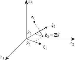
The geometric analysis in Figure 2.2 confirms the result in (2.3), since
where ![]() is the angle between z0 and
is the angle between z0 and ![]() . Given that
. Given that ![]() , reformulating (2.3) yields
, reformulating (2.3) yields
Figure 2.2 Orthogonal projection of z0 onto orthonormal column vector of Ξ.
The projection of a sample onto the column vectors of Ξ is given by
2.6 ![]()
The estimation of s, however, does not reduce to the simple projection shown in (2.4) and (2.5) if the column vectors of Ξ are not mutually orthonormal. To address this, PCA determines nz orthonormal loading vectors such that n of them span the same column space as Ξ, which are stored as column vectors in the matrix ![]() . The remaining nz − n loading vectors are stored in the matrix
. The remaining nz − n loading vectors are stored in the matrix ![]() . These two matrices have the following orthogonality properties
. These two matrices have the following orthogonality properties
2.7 
The loading vectors are eigenvectors of ![]() and the above orthogonality properties give rise to the calculation of the following orthogonal projections
and the above orthogonality properties give rise to the calculation of the following orthogonal projections
2.8 
The ith element stored in ![]() represents the coordinate describing the orthogonal projection of z0 onto the ith column vector in P. Note that the column space of P is identical to the column space of Ξ. Moreover, the column vectors of P and Pd are base vectors spanning the model subspace and the residual subspace, respectively.
represents the coordinate describing the orthogonal projection of z0 onto the ith column vector in P. Note that the column space of P is identical to the column space of Ξ. Moreover, the column vectors of P and Pd are base vectors spanning the model subspace and the residual subspace, respectively.
Given that the column vectors stored in Pd are orthogonal to those in P, they are also orthogonal to those in Ξ. Consequently, ![]() . In this regard, the jth element of td is equal to the coordinate describing the orthogonal projection of z0 onto the jth column vector in Pd. In other words, the elements in t are the coordinates describing the orthogonal projection of z0 onto the model subspace and the elements in td are the coordinates describing the orthogonal projection of z0 onto the residual subspace. This follows from the geometric analysis in Figure 2.2.
. In this regard, the jth element of td is equal to the coordinate describing the orthogonal projection of z0 onto the jth column vector in Pd. In other words, the elements in t are the coordinates describing the orthogonal projection of z0 onto the model subspace and the elements in td are the coordinates describing the orthogonal projection of z0 onto the residual subspace. This follows from the geometric analysis in Figure 2.2.
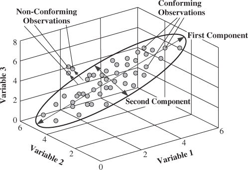
On the basis of the preceding discussion, Figure 2.3 shows an extension of the simple 2-variable example to a 3-variable one, where two common cause ‘source’ variables describe the variation of 3 process variables. This implies that the dimensions of the model and residual subspaces are 2 and 1, respectively.
Figure 2.3 Schematic diagram of showing the PCA model subspace and its complementary residual subspace for 3 process variables.
2.1.3 A simulation example
Using the geometric analysis in Figure 2.3, this example shows how to obtain an estimate of the model subspace ![]() and the residual subspace, defined by the cross product of
and the residual subspace, defined by the cross product of ![]() and
and ![]() . The data model for this example is
. The data model for this example is
2.9 
which has a mean vector of zero. The elements in s follow a Gaussian distribution
2.10 
The error vector ![]() contains random variables that follow a Gaussian distribution too
contains random variables that follow a Gaussian distribution too
2.11 ![]()
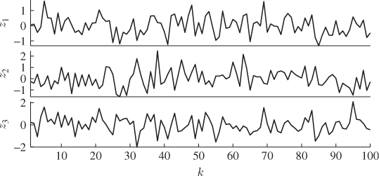
From this process, a total of K = 100 samples, z0(1), … , z0(k), … , z0(100) are simulated. Figure 2.4 shows time-based plots for each of the 3 process variables. PCA analyzes the stochastic variation encapsulated within this reference set, which leads to the determination of the model subspace, spanned by the column vectors of Ξ, and the complementary residuals subspace. Chapter 9 highlights that this involves the data covariance matrix, which must be estimated from the recorded data
2.12 
Figure 2.4 Time-based plot of simulated process variables.
For a nonzero mean vector, it must be estimated from the available samples first
which yields the following estimation of the data covariance matrix
The estimation of the data covariance matrix from the recorded reference data is followed by determining its eigendecomposition
which produces the following estimates for the eigenvector and eigenvalue matrices
2.16 
and
2.17 
respectively.
Given that Ξ, Sss and ![]() are known, the covariance matrix for the recorded variables can be determined as shown in Table 2.1
are known, the covariance matrix for the recorded variables can be determined as shown in Table 2.1
2.18 
Subsection 6.1 points out that ![]() asymptotically converges to
asymptotically converges to ![]() . To examine how accurate the PCA model has been estimated from K = 100 samples, the eigendecomposition of
. To examine how accurate the PCA model has been estimated from K = 100 samples, the eigendecomposition of ![]() can be compared with that of
can be compared with that of ![]()
2.19 
The departures of the estimated eigenvalues are:
 ;
; ; and
; and .
.
To determine the accuracy of the estimated model subspace, we can compare the normal vector of the actual model subspace with the estimated one. The one for the model subspace is proportional to the cross product, denoted here by the symbol × , of the two column vectors of Ξ
2.20 
As the simulated process has two normally distributed source signals, the two principal components associated with the two largest eigenvalues must, accordingly, be associated with the model subspace, whilst the third one represents the complementary residual subspace, spanned by the third eigenvector. This is based on the fact that the eigenvectors are mutually orthonormal, as shown in Chapter 9. The last column of the matrix ![]() stores the third eigenvector and the scalar product of this vector with n yields the minimum angle between the true and estimated residual subspace
stores the third eigenvector and the scalar product of this vector with n yields the minimum angle between the true and estimated residual subspace
Equation (2.21) shows that the estimated model subspace is rotated by just over 2° relative to the actual one. In contrast, the one determined from ![]() , as expected, is equal to n.
, as expected, is equal to n.
Figure 2.2 shows that storing the 100 samples consecutively as row vectors in the matrix ![]() allows determining the orthogonal projection of these samples onto the estimated model subspace as follows
allows determining the orthogonal projection of these samples onto the estimated model subspace as follows
2.22 ![]()
where ![]() and
and ![]() store the coordinates that determine the location of samples when projected orthogonally onto
store the coordinates that determine the location of samples when projected orthogonally onto ![]() and
and ![]() , respectively.
, respectively.
It should be noted that even if the column vectors of Ξ are orthonormal they may be different to the eigenvectors of ![]() . This is because PCA determines the principal directions such that the orthogonal projection of z0 produces a maximum variance for each of them. More precisely,
. This is because PCA determines the principal directions such that the orthogonal projection of z0 produces a maximum variance for each of them. More precisely, ![]() , which is equal to
, which is equal to ![]() , and follows from the analysis of PCA in Chapter 9. These expectations, however, are equal to the eigenvalues of
, and follows from the analysis of PCA in Chapter 9. These expectations, however, are equal to the eigenvalues of ![]() , which, accordingly, represent the variances of the projections, i.e. the t-scores or principal components such that λ1 ≥ λ2 ≥ ··· ≥ λn.
, which, accordingly, represent the variances of the projections, i.e. the t-scores or principal components such that λ1 ≥ λ2 ≥ ··· ≥ λn.
Another aspect that this book discusses is the use of scatter diagrams for the loading vectors. Figure 1.9 shows a scatter diagram for two highly correlated variables. Moreover, Subsection 3.1.1 introduces scatter diagrams and the construction of the control ellipse, or ellipsoid if the dimension exceeds 2, for the score variables or principal components. Scatter diagrams for the loading vectors, on the other hand, plot the elements of the pairs or triples of loading vectors, for example the ith and the jth loading vector. This allows identifying groups of variables that have a similar covariance structure. An example and a detailed discussion of this is available in Kaspar and Ray (1992). The application studies in Chapters 4 and 5 also present a brief analysis of the variable interrelationships for recorded data sets from a chemical reaction and a distillation process, respectively.
2.2 Partial least squares
As in the previous section, the presentation of PLS relies on a geometric analysis. Chapter 10 provides a more detailed analysis of the PLS algorithm, including its properties and further information is available from the research literature, for example (de Jong 1993; de Jong et al. 2001; Geladi and Kowalski 1986; Höskuldsson 1988; Lohmoeller 1989; ter Braak and de Jong 1998). In contrast to PCA, PLS relies on the analysis of two variable sets that represent the process input and output variable sets shown in Figure 2.5. Alteratively, these variable sets are also referred to as the predictor and response, the cause and effect, the independent and dependent or the regressor and regressand variables sets in the literature. For simplicity, this book adopts the notation input and output variable sets to denote ![]() as the input and
as the input and ![]() as the output variable sets. These sets span separate data spaces denoted as the input and output spaces, which Figure 2.5 graphically illustrates.
as the output variable sets. These sets span separate data spaces denoted as the input and output spaces, which Figure 2.5 graphically illustrates.
Figure 2.5 Division of the process variables into input and output variables.
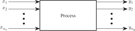
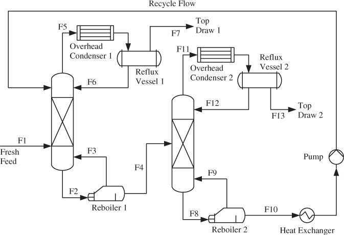
Figure 2.6 Schematic diagram of a distillation unit.
Between these variables sets, there is the following linear parametric relationship
where x0 and y0 are zero mean random vectors that follow a Gaussian distribution. Similar to (2.2), the recorded variables are defined by ![]() and
and ![]() with
with ![]() and
and ![]() being mean vectors. The matrix
being mean vectors. The matrix ![]() is a parameter matrix describing the linear relationships between x0 and the uncorrupted output variables
is a parameter matrix describing the linear relationships between x0 and the uncorrupted output variables ![]() , and
, and ![]() is an error vector, representing measurement uncertainty for the output variables or the impact of unmeasured disturbances for example.
is an error vector, representing measurement uncertainty for the output variables or the impact of unmeasured disturbances for example.
The error vector ![]() is also assumed to follow a zero mean Gaussian distribution and is statistically independent of the input vector x0, implying that
is also assumed to follow a zero mean Gaussian distribution and is statistically independent of the input vector x0, implying that ![]() . Moreover, the covariance matrices for x0, ys and
. Moreover, the covariance matrices for x0, ys and ![]() are
are ![]() ,
, ![]() and
and ![]() , respectively. To denote the parametric matrix
, respectively. To denote the parametric matrix ![]() by its transpose relates to the identification of this matrix from recorded samples of x and y which are stored as row vectors in data matrices. This is discussed further in Chapter 10.
by its transpose relates to the identification of this matrix from recorded samples of x and y which are stored as row vectors in data matrices. This is discussed further in Chapter 10.
2.2.1 Assumptions for underlying data structure
With respect to the preceding discussion, the recorded variables are highly correlated. Separating them into the mean centered input and output variable sets implies that the individual sets are also highly correlated. According to (2.23), there is also considerable correlation between the input and output variables:
- as the uncorrupted output variables are a linear combination of the input variables; and
- the assumption that
 for all 1 ≤ i ≤ nx, where
  is the ith column vector of
  .
.
To illustrate the correlation issue in more detail, consider the distillation process in Figure 2.6. The output variables of this process are mainly tray temperature, pressure and differential pressure measurements inside the columns, and concentrations (if measured). These variables follow common cause variation, for example introduced by variations of the fresh feed and its composition as well as the temperatures and flow rate of the input streams into the reboilers and overhead condensers. Other sources that introduce variation are, among others, unmeasured disturbances, changes in ambient temperature and pressure, and operator interventions. Through controller feedback, the variations of the output variables will propagate back to the input variables, which could include flow rates, temperatures of the heating/cooling streams entering and leaving the reboilers and overhead condensers. The degree of correlation within both variable sets suggests the following data structure for the input and output variables
Here, ![]() and
and ![]() are parameter matrices,
are parameter matrices, ![]() and
and ![]() are the residual vectors of the input and output sets, respectively, which describe a negligible contribution for predicting the output set. The vector s stores the source signals describing common cause variation of the input and output sets. Recall that
are the residual vectors of the input and output sets, respectively, which describe a negligible contribution for predicting the output set. The vector s stores the source signals describing common cause variation of the input and output sets. Recall that ![]() is the error vector associated with the output variables and
is the error vector associated with the output variables and ![]() under the assumptions (i) that the covariance matrix of the input variables has full rank nx, (ii) that n = nx and (iii) that the number of samples for identifying the PLS model in (2.24) K → ∞.
under the assumptions (i) that the covariance matrix of the input variables has full rank nx, (ii) that n = nx and (iii) that the number of samples for identifying the PLS model in (2.24) K → ∞.
The source and error signals are assumed to be statistically independent of each other and follow a zero mean Gaussian distribution
2.25 
Moreover, the residual vectors e and f are also assumed to follow zero mean Gaussian distributions with covariance matrices See and Sff, respectively. The residual vectors, however, are generally not statistically independent, i.e. E{efT} ≠ 0. Subsection 2.3.2 discusses the independence of the error vectors in more detail. Asymptotically, if n = nx and K → ∞, however, ![]() and See → 0.
and See → 0.
By comparing the causal data model for PLS with that of the non-causal PCA one in (2.2), it should be noted that there are similarities. The parameter matrix Ξ for the PCA data model becomes ![]() and
and ![]() to describe the influence of the source variables upon the input and output variables, respectively. Moreover, the error variable g for the PCA data structure becomes e and f for the input and output variable sets, respectively. For PCA, however, if the number of source signals is assumed to be n = nz, the variable set z0 can be described by
to describe the influence of the source variables upon the input and output variables, respectively. Moreover, the error variable g for the PCA data structure becomes e and f for the input and output variable sets, respectively. For PCA, however, if the number of source signals is assumed to be n = nz, the variable set z0 can be described by ![]() . This follows from the fact that the covariance matrix of z0 is equal to its eigendecomposition for n = nz, as shown in (2.15) for
. This follows from the fact that the covariance matrix of z0 is equal to its eigendecomposition for n = nz, as shown in (2.15) for ![]() . With regards to PLS, however, this property is only maintained for the input variable set x0, as e → 0 for n → nx. In contrast, as n → nx the error vector
. With regards to PLS, however, this property is only maintained for the input variable set x0, as e → 0 for n → nx. In contrast, as n → nx the error vector ![]() .
.
Using the terminology for training artificial neural networks in an MSPC context, assuming that the variable sets z0 and x0 are identical PCA is an unsupervised learning algorithm for determining latent variable sets. In contrast, PLS is a supervised learning algorithm, which incorporates the parametric relationship relationship ![]() into the extraction of sets of latent variables. Although this comparison appears hypothetical, this is a practically relevant case. An example is if the output variable set y0 consists of concentration measurements that represent quality variables which are not recorded with the same frequency as the variable set x0. In this case, only the z0 = x0 is available for on-line process monitoring.
into the extraction of sets of latent variables. Although this comparison appears hypothetical, this is a practically relevant case. An example is if the output variable set y0 consists of concentration measurements that represent quality variables which are not recorded with the same frequency as the variable set x0. In this case, only the z0 = x0 is available for on-line process monitoring.
2.2.2 Deflation procedure for estimating data models
PLS computes sequences of linear combinations of the input and output variables to determine sets of latent variables that describe common cause variation. The first set of latent variables includes
2.26 ![]()
where w1 and q1 are weight vectors of unit length that determine a set of linear combinations of x0 and y0, respectively, and yield the score variables t1 and u1. Geometrically, the linear combinations result in the orthogonal projections of the data vectors x0 and y0 onto the directions defined by w1 and q1, respectively. This follows from the fact that ![]() and
and ![]() are scalar products
are scalar products
2.27 ![]()
and
2.28 ![]()
where ![]() and
and ![]() are the angles between the vector pairs x0 and w1, and y0 and q1, respectively. Consequently, the score variables t1 and u1 describe the minimum distance between the origin of the coordinate system and the orthogonal projection of x0 and y0 onto w1 and q1, respectively. The weight vectors are determined to maximize the covariance between t1 and u1.
are the angles between the vector pairs x0 and w1, and y0 and q1, respectively. Consequently, the score variables t1 and u1 describe the minimum distance between the origin of the coordinate system and the orthogonal projection of x0 and y0 onto w1 and q1, respectively. The weight vectors are determined to maximize the covariance between t1 and u1.
Chapter 10 gives a detailed account of the PLS objective functions for computing the weight vectors. After determining the score variables, the t-score variable is utilized to predict the input and output variables. For this, PLS computes a set of loading vectors, leading to the following prediction of both variable sets
2.29 ![]()
Here, p1 and ![]() are the loading vectors for the input and output variables, respectively. As before, the notation
are the loading vectors for the input and output variables, respectively. As before, the notation ![]() represents the prediction or estimation of a variable. Chapter 10, again, shows the objective function for determining the loading vectors. The aim of this introductory section on PLS is to outline its working and how to apply it.
represents the prediction or estimation of a variable. Chapter 10, again, shows the objective function for determining the loading vectors. The aim of this introductory section on PLS is to outline its working and how to apply it.
It should be noted, however, that the weight and the loading vector of the output variables, q1 and ![]() , are equal up to a scalar factor. The two weight vectors, w1 and q1, the two loading vectors, p1 and
, are equal up to a scalar factor. The two weight vectors, w1 and q1, the two loading vectors, p1 and ![]() , and the two score variables, t1 and u1 are referred to as the first set of latent variables (LVs). For computing further sets, the PLS algorithm carries out a deflation procedure, which subtracts the contribution of previously computed LVs from the input and output variables. After computing the first set of LVs, the deflation procedure yields
, and the two score variables, t1 and u1 are referred to as the first set of latent variables (LVs). For computing further sets, the PLS algorithm carries out a deflation procedure, which subtracts the contribution of previously computed LVs from the input and output variables. After computing the first set of LVs, the deflation procedure yields
2.30 ![]()
where e2 and f2 are residual vectors that represent variation of the input and output variable sets which can be exploited by the second set of LVs, comprising of the weight vectors w2 and q2, the loading vectors p2 and ![]() and the score variables t2 and u2. Applying the deflation procedure again yields
and the score variables t2 and u2. Applying the deflation procedure again yields
2.31 ![]()
Defining the original data vectors x0 and y0 as e1 and f1, the general formulation of the PLS deflation procedure becomes
2.32 ![]()
and the ith pair of LVs include the weight vectors wi and qi, the loading vectors pi and ![]() and the score variables ti and ui.
and the score variables ti and ui.
Compared to the data structure in (2.24), the objective of the PLS modeling procedure is to:
- estimate the column space of parameter matrices
 and
and  ; and
; and - extract the variation of the source variable set s.
From the n sets of LVs, the p- and ![]() -loading vectors, stored in separate matrices
-loading vectors, stored in separate matrices
2.33 ![]()
are an estimate for the column space of ![]() and
and ![]() . The t-score variables
. The t-score variables
2.34 ![]()
represent the variation of the source variables.
2.2.3 A simulation example
To demonstrate the working of PLS, an application study of data from a simulated process is now presented. According to (2.23), the process includes three input and two output variables and the following parameter matrix
The input variable set follows a zero mean Gaussian distribution with a covariance

The error variable set, ![]() follows a zero mean Gaussian distribution describing i.i.d. sequences
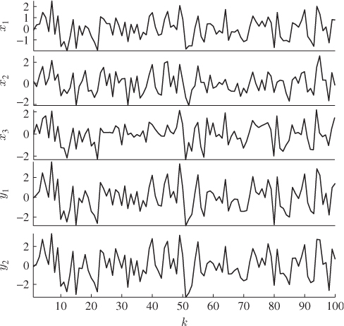
follows a zero mean Gaussian distribution describing i.i.d. sequences ![]() . Figure 2.7 shows a total of 100 samples, that were simulated from this process, and produced the following covariance matrices
. Figure 2.7 shows a total of 100 samples, that were simulated from this process, and produced the following covariance matrices
2.37 
Figure 2.7 Simulated samples of input and output variables.
Equations 2.38 and 2.39 show how to compute the cross-covariance matrix
or
If ![]() and
and ![]() are equal to zero, the estimation of the covariance and cross-covariance matrices requires the use of (2.13) and (2.38). If this is not the case for at least one of the two variable sets, use (2.14) and (2.38) to estimate them.
are equal to zero, the estimation of the covariance and cross-covariance matrices requires the use of (2.13) and (2.38). If this is not the case for at least one of the two variable sets, use (2.14) and (2.38) to estimate them.
Knowing that ![]() is statistically independent of x0, (2.23) shows that these covariance matrices
is statistically independent of x0, (2.23) shows that these covariance matrices ![]() and
and ![]() are equal to
are equal to
and
respectively. Inserting ![]() ,
, ![]() and
and ![]() , defined in (2.35) and (2.36), into (2.40) and (2.41) yields
, defined in (2.35) and (2.36), into (2.40) and (2.41) yields
2.42 
Comparing the true matrices with their estimates shows a close agreement.
Using the estimated matrices ![]() and
and ![]() , a PLS model is determined next. The preceding discussion has outlined that a PLS model relies on the calculation of weight vectors of length 1. The projection of the input and output variables onto these weight vectors then produces the score variables. To complete the computation of one set of latent variables, the final step is to determine the loading vectors and the application of the deflation procedure to the input and output variables.
, a PLS model is determined next. The preceding discussion has outlined that a PLS model relies on the calculation of weight vectors of length 1. The projection of the input and output variables onto these weight vectors then produces the score variables. To complete the computation of one set of latent variables, the final step is to determine the loading vectors and the application of the deflation procedure to the input and output variables.
Figure 2.8 illustrates the working of the iterative PLS approach to the input and output data shown in Figure 2.7. The left and right column of plots present the results for the individual sets of latent variables, respectively. The top, middle and bottom rows of plots summarize the results of the first, the second and the third sets of latent variables, respectively. The first set of latent variables are computed from the original input and output variable sets and the first two plots at the top show the samples and the computed direction of the weight vectors.
Figure 2.8 Graphical illustration of the sample projections in the input and output spaces for determining the first, second and third set of latent variables.
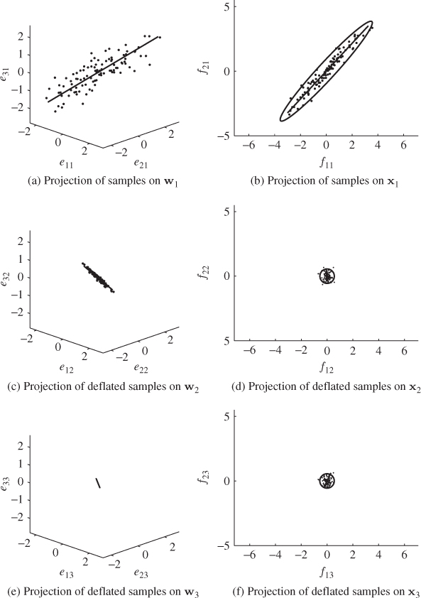
The control ellipses in the right plots are for the two output variables. The depicted samples in the middle and lower rows of plots represent the samples after the first and second deflation procedure has been carried out. It is interesting to note that after applying the first deflation procedure to the output variables, there is little variation left in this variable set, noticeable by the small control ellipse constructed on the basis of the covariance matrix of ![]() . The deflation procedure also reduces the remaining variation of the input variables when comparing the top left with the middle left plot.
. The deflation procedure also reduces the remaining variation of the input variables when comparing the top left with the middle left plot.
The third and final set of LVs is determined from the input and output variable sets after deflating the first and second sets of LVs. Comparing the plots in the bottom row with those in the middle of Figure 2.8 suggests that there is hardly any reduction in the remaining variance of the output variables but a further reduction in variation of the input variables. The analysis in Chapter 10 shows that after deflating the third set of latent variables from the input and output variables, the residuals of the input variable set is zero and the residuals of the output variables are identical to those of applying a regression model obtained from the ordinary least squares (OLS). Asymptotically, the residuals f converge to ![]() as K → ∞.
as K → ∞.
Equation 2.43 lists the estimates for the w- and q-weight, the p- and ![]() -loading matrices and the maximum covariance values for the t- and u-score variables
-loading matrices and the maximum covariance values for the t- and u-score variables
Using the true covariance matrices, it is possible to compare the accuracy of the estimated ones. It follows from the analysis in Chapter 10 that each LV in one set can be computed either from the w- or the q-weight vector. It is therefore sufficient to determine the departure of the estimated w-weight vectors. The estimation error of the other LVs can be computed from the estimation error of the covariance matrices and the w-weight vector. For example, the estimation error for the q-weight vector is
2.44 
It is assumed here that ![]() ,
, ![]() and
and ![]()
![]() . The true w-weight matrix is equal to
. The true w-weight matrix is equal to
2.45 
Since the w-weight vectors are of unit length, the angles between the estimated and true ones can directly be obtained using the scalar product ![]() and are 0.2374°, 0.6501° and 0.6057° for the first, second and third vectors, respectively. The covariances of the first, the second and the third pair of score variables, obtained from the true covariance matrices, are 3.2829, 0.1296 and 0.0075 respectively, and close to the estimated ones stored in the vector
and are 0.2374°, 0.6501° and 0.6057° for the first, second and third vectors, respectively. The covariances of the first, the second and the third pair of score variables, obtained from the true covariance matrices, are 3.2829, 0.1296 and 0.0075 respectively, and close to the estimated ones stored in the vector ![]() in (2.43). The estimation error for the w-weight vectors are around 0.25° for the first and around 0.65° for the second and third ones and is therefore small. The estimation accuracy, however, increases with the number of recorded samples. After inspecting the estimation accuracy, a very important practical aspect, namely how to interpret the results obtained, is given next.
in (2.43). The estimation error for the w-weight vectors are around 0.25° for the first and around 0.65° for the second and third ones and is therefore small. The estimation accuracy, however, increases with the number of recorded samples. After inspecting the estimation accuracy, a very important practical aspect, namely how to interpret the results obtained, is given next.
So far, the analysis of the resultant PLS regression model has been made from Figure 2.8 by eye, for example, noticing that the number of samples outside the control ellipse describing the error vector ![]() . A sound statistically-based conclusions, however, requires a more detailed investigation. For example, such an analysis helps in determining how many sets of latent variables need to be retained in the PLS model and how many sets can be discarded. One possibility to assess this is the analysis of the residual variance, given in Table 2.2.
. A sound statistically-based conclusions, however, requires a more detailed investigation. For example, such an analysis helps in determining how many sets of latent variables need to be retained in the PLS model and how many sets can be discarded. One possibility to assess this is the analysis of the residual variance, given in Table 2.2.
Table 2.2 Variance reduction of PLS model to x0 and y0.
| LV Set | Input Variables x0 ( |
Output Variables y0 ( |
| 1 | 17.3808% | 3.1522% |
| 2 | 0.5325% | 2.1992% |
| 3 | 0.0000% | 2.0875% |
The percentage values describe the cumulative variance remaining.
Equation (2.46) introduces a measure for the residual variance of both variable sets, ![]() and
and ![]() , after deflating the previously computed i − 1 LVs
, after deflating the previously computed i − 1 LVs
where trace{ · } is the sum of the diagonal elements of a squared matrix,
2.47 
and
2.48 
The assumption that the process variables are normally distributed implies that the t-score variables ![]() are statistically independent, which the analysis in Chapter 10 yields. Hence,
are statistically independent, which the analysis in Chapter 10 yields. Hence, ![]() reduces to a diagonal matrix.
reduces to a diagonal matrix.
Summarizing the results in Table 2.2, the first set of LVs contribute to a relative reduction in variance of 82.6192% for the input and 96.8478% for the output variable set. For the second set of LVs, a further relative reduction of 16.8483% can be noticed for the input variable set, whilst the reduction for the output variables only amounts to 0.9530%. Finally, the third set of LVs only contribute marginally to the input and output variables by 0.5225% and 0.1117%, which is negligible.
The analysis in Table 2.2 therefore confirms the visual inspection of Figure 2.8. Given that PLS aims to determine a covariance representation of x0 and y0 using a reduced set of linear combinations of these sets, a parsimonious selection is to retain the first set of LVs and discard the second and third sets as insignificant contributors.
The final analysis of the PLS model relates to the accuracy of the estimated parameter matrix, ![]() . Table 2.2 shows that x0 is completely exhausted after deflating 3 sets of LVs. Furthermore, the theoretical value for
. Table 2.2 shows that x0 is completely exhausted after deflating 3 sets of LVs. Furthermore, the theoretical value for ![]() can be obtained
can be obtained
2.49 ![]()
As stated in the preceding discussion, the estimated regression matrix, including all three sets of LVs, is equivalent to that obtained using the OLS approach. Equation (2.50) shows this matrix from the simulated 100 samples
Comparing the estimated parameter matrix with the true one, shown in (2.35), it should be noted that particularly the first column of ![]() departs from
departs from ![]() , whilst the second column provides a considerably closer estimate. Larger mismatches between the estimated and true parameter matrix can arise if:
, whilst the second column provides a considerably closer estimate. Larger mismatches between the estimated and true parameter matrix can arise if:
- there is substantial correlation among the input variables (Wold et al. 1984); and
- the number of observations is ‘small’ compared to the number of variables (Ljung 1999; Söderström and Stoica 1994).
By inspecting the ![]() in (2.36), non-diagonal elements of 0.9 and 0.8 show indeed a high degree of correlation between the input variables. Subsection 6.2.1 presents a further and more detailed discussion of the issue of parameter identification. The issue related to the accuracy of the PLS model is also a subject in the Tutorial Session of this chapter and further reading material covering the aspect of model accuracy is given in Höskuldsson (1988, 1996).
in (2.36), non-diagonal elements of 0.9 and 0.8 show indeed a high degree of correlation between the input variables. Subsection 6.2.1 presents a further and more detailed discussion of the issue of parameter identification. The issue related to the accuracy of the PLS model is also a subject in the Tutorial Session of this chapter and further reading material covering the aspect of model accuracy is given in Höskuldsson (1988, 1996).
2.3 Maximum redundancy partial least squares
This section examines the legitimate question of why do we need both, the single-block PCA and the dual-block PLS methods for process monitoring. A more precise formulation of this question is: what can the separation of the recorded variable set to produce a dual-block approach offer that a single-block technique cannot? To address this issue, the first subsection extends the data models describing common cause variation in (2.2) and (2.24). Subsection 2.3.2 then shows that PCA and PLS cannot identify this generic data structure correctly. Finally, Subsection 2.3.3 introduces a different formulation of the PLS objective function that enables the identification of this generic data structure, and Subsection 2.3.4 presents a simulation example to demonstrate the working of this revised PLS algorithm.
2.3.1 Assumptions for underlying data structure
The preceding discussion in this chapter has outlined that PCA is a single-block technique that analyzes a set of variables. According to (2.2), this variable set is a linear combination of a smaller set of source signals that represent common cause variation. For each process variable, a statistically independent error variable is then superimposed to the contribution from the source signals.
On the other hand, PLS is a dual-block technique for which the recorded variables are divided into an input and an output set. Figure 2.6 shows that this division may not be straightforward. Whilst the fresh feed (stream F1) is easily identified as an input and top draw 1 (stream F7) and top draw 2 (stream F14) are outputs, how can the remaining streams (flow rates), temperature variables, pressure measurements, differential pressures or concentrations (if measured on-line) be divided?
An approach that the literature has proposed is selecting the variables describing the product quality as the outputs and utilizing the remaining ones as ‘inputs’. This arrangement separates the variables between a set of cause variables that describe, or predict, the variation of the output or effect variables. A question that one can justifiably ask is why do we need PLS if PCA is able to analyze a single-block arrangement of these variables, which is conceptually simpler? In addition to that, the division into input and output variables may not be straightforward either.
The need for a dual-block technique becomes clear by revisiting Figure 2.6. The concentrations (the quality variables y0), are influenced by changes affecting the energy balance within the distillation towers. Such changes manifest themselves in the recorded temperatures and pressures for example. On the other hand, there are also variables that relate to the operation of reboilers 1 and 2, overhead condensers 1 and 2, both reflux vessels, the heat exchanger and the pump that do not affect the quality variables. The variation in these variables, however, may be important to monitor the operation of the individual units and consequently cannot be ignored.
A model to describe the above scenario is an extension of (2.24)
where s represents common cause variation in both variable sets and s′ describes variation among the input or cause variables that is uncorrelated to the output variables and hence, uninformative for predicting them. The next subsection examines whether PCA and PLS can identify the data structure in (2.51).
2.3.2 Source signal estimation
The model estimation w.r.t. (2.51) is separately discussed for PCA/PLS.
2.3.2.1 Model identification using PCA
The advantage of a dual block method over a single block approach, when applied to the above data structure, is best demonstrated by reformulating (2.51)
Now, applying PCA to the data structure in (2.52) yields the following estimate for the source signals and residuals
2.53 ![]()
and
2.54 ![]()
respectively. Here, P and Pd store the first n and the remaining nz − n eigenvectors of the data covariance matrix ![]() , respectively, where
, respectively, where
2.55 
Note that above covariance matrix is divided into a part that represents common cause variation and a second part that describes the common cause variation that only affects input variables and the error term for the output variables. Assuming that the model subspace, spanned by the eigenvectors stored in P is consistently estimated,2 the elements in ![]() are linear combinations of
are linear combinations of ![]() . Consequently, it may not be possible to extract and independently monitor
. Consequently, it may not be possible to extract and independently monitor ![]() using PCA.
using PCA.
Moreover, the covariance matrix ![]() is not known a priori and may have significantly larger entries compared to the error covariance matrix
is not known a priori and may have significantly larger entries compared to the error covariance matrix ![]() . It is also possible that
. It is also possible that ![]() is the dominant contribution of the joint variable set z0. Both aspects render the estimation of the column space
is the dominant contribution of the joint variable set z0. Both aspects render the estimation of the column space ![]() using PCA a difficult task, given that the error covariance matrix is not of the form
using PCA a difficult task, given that the error covariance matrix is not of the form ![]() . More precisely, Subsection 6.1.1 discusses how to estimate the error covariance matrix and the model subspace simultaneously using maximum likelihood PCA.
. More precisely, Subsection 6.1.1 discusses how to estimate the error covariance matrix and the model subspace simultaneously using maximum likelihood PCA.
Based on this simultaneous estimate, the source signals contribution ![]() must be considered as additional error variables that:
must be considered as additional error variables that:
- may have a considerably larger variance and covariance values compared to those of
 ; and
; and - the rank of the covariance matrix
 is nx − n and not nx.
The assumption for estimating the error covariance matrix, however, is that it is a full rank matrix. Hence, PCA is (i) unable to separate the source signals of the input variables into those commonly shared by the input and output variables, and the remaining ones that are only encapsulated in the input variables and (ii) unable to identify the data structure using a maximum likelihood implementation.
2.3.2.2 Model Identification Using PLS
Different from PCA, PLS extracts t-score variables from the input variables. It is therefore tempting to pre-conclude that PLS extracts common cause variation by determining the n t-score variables that discard the non-predictive variation in ![]() . The fact that the cross-covariance matrix
. The fact that the cross-covariance matrix ![]() does not represent the signal contributions
does not represent the signal contributions ![]() and
and ![]() reinforces this assumption.
reinforces this assumption.
A more detailed analysis, however, yields that this is not the case. Equation 2.56 reexamines the construction of the weight vectors assuming that q is predetermined
The score variables are linear combination of x0 and y0, which implies that
Equation 2.57 dictates the condition for separating s and s′ is ![]() . Applying 1.8 to reformulate the covariance of the pair of score variables yields
. Applying 1.8 to reformulate the covariance of the pair of score variables yields

where rtu is the correlation coefficient between the score variables. If ![]() , it follows from (2.58) that
, it follows from (2.58) that
2.59 
and hence, the t-score variable does not include the non-predictive contribution ![]() . This, however, generally cannot be assumed. It therefore follows that PCA and PLS cannot estimate a model that discriminates between:
. This, however, generally cannot be assumed. It therefore follows that PCA and PLS cannot estimate a model that discriminates between:
- the common cause variation of the input and output variables;
- the non-predictive variation encapsulated in the input variables only; and
- the error variables corrupting the outputs.
The next subsection develops an alternative PLS formulation that extracts the common cause variation and discriminates between the three different types of variation.
2.3.3 Geometric analysis of data structure
The detailed examination of (2.56) to (2.58) yields that PLS effectively does not produce score variables that are related to model accuracy. This follows from the fact that the covariance criterion can be expressed by the product of the correlation coefficient times the square root of the variance products of the score variable. A larger variance for any of the score variables at the expense of a smaller correlation coefficient may, consequently, still produce a larger covariance. Model accuracy in the score space, however, is related to the correlation coefficient. The larger the correlation coefficient between two variables the more they have in common and hence, the more accurately one of these variables can predict the other.
Preventing PLS from incorporating P′s′ into the calculation of the t-score variables requires, therefore, a fresh look at its objective function. As outlined above, the key lies in determining weight vectors based on an objective function that relates to model accuracy rather than covariance. Starting with the following data structure

for which the best linear unbiased estimator is the OLS solution (Henderson 1975)
Using (2.60) and (2.61) gives rise to reformulate ![]() as follows
as follows
2.62 ![]()
where ![]() . It follows from (2.60) that the only contribution to
. It follows from (2.60) that the only contribution to ![]() that can be predicted by the linear model is
that can be predicted by the linear model is ![]() , since
, since ![]() . In a similar fashion to PCA, it is possible to determine a direction vector to maximize the following objective function
. In a similar fashion to PCA, it is possible to determine a direction vector to maximize the following objective function
where ![]() . The optimal solution for (2.63) is
. The optimal solution for (2.63) is
The eigenvalue λ is the variance of the orthogonal projection of ![]() onto q. The solution to (2.64) is the eigenvector associated with the largest eigenvalue of
onto q. The solution to (2.64) is the eigenvector associated with the largest eigenvalue of ![]() . The eigenvector associated with the second largest eigenvalue captures the second largest contribution and so on.
. The eigenvector associated with the second largest eigenvalue captures the second largest contribution and so on.
Whilst this allows to extract weight vectors for y0, how to determine weight vectors for x0 to predict the u-score variable ![]() as accurately as possible? By revisiting (2.57) and (2.58) it follows that the correlation coefficient rtu must yield a maximum to achieve this
as accurately as possible? By revisiting (2.57) and (2.58) it follows that the correlation coefficient rtu must yield a maximum to achieve this
where ![]() and t = wTx0. By incorporating the constraint
and t = wTx0. By incorporating the constraint ![]() , setting the variance of wTx0 to be 1,
, setting the variance of wTx0 to be 1, ![]() and (2.65) becomes
and (2.65) becomes
The fact that λ = E{(qTy0)2} follows from
 ,
, , and
, and ,
,
so that ![]() . The objective function in (2.66) therefore maximizes the correlation coefficient,
. The objective function in (2.66) therefore maximizes the correlation coefficient, ![]() , and has the following solution
, and has the following solution
2.67 ![]()
where the Lagrangian multiplier, μ, satisfies the constraint ![]() . Next, (2.63) and (2.66) can be combined to produce the objective function
. Next, (2.63) and (2.66) can be combined to produce the objective function
which has the following solution for w and q
2.69 ![]()
and hence
That both Lagrangian multiples have the same value follows from
2.71 ![]()
This solution relates to a nonsymmetric index of redundancy, introduced by Stewart and Love (1968) to describe the amount of predicted variance, and was first developed by van den Wollenberg (1977). Moreover, ten Berge (1985) showed that van den Wollenberg's maximum redundancy analysis represents a special case of Fortier's simultaneous linear prediction (Fortier 1966). The objective of the work in Fortier (1966) is to determine a linear combination of a set of predictors (inputs) that has a maximum predictability for all predictants (outputs) simultaneously.
The next step is to apply the standard PLS deflation procedure to determine subsequent sets of LVs. According to the data model in (2.51), only the contribution Ps in x0 is predictive for y0. By default, the solution of the objective function in (2.68) must discard the contribution P′s′. The next question is how many sets of latent variables can be determined by solving (2.68) and carrying out the PLS deflation procedure? The answer to this lies in the cross covariance matrix ![]() as it only describes the common cause variation, that is,
as it only describes the common cause variation, that is, ![]() .
.
The loading vectors pi and ![]() can now be computed by
can now be computed by
Utilizing (2.72), the deflation of the covariance matrix is
2.73 ![]()
and similarly for the cross-covariance matrix
If the cross-covariance matrix is exhausted, there is no further common cause variation in the input variable set. One criterion for testing this, or a stopping rule according to the next section, would be to determine the Frobenius norm of the cross-covariance matrix after applying the ith deflation procedure
If (2.75) is larger than zero, obtain the (i + 1)th pair of weight vectors, wi+1 and qi+1, by solving (2.70). On the other hand, if (2.75) is zero, the common cause variation has been extracted from the input variables.
It is important to note that (2.70) presents an upper limit for determining the maximum number of weight vector pairs. Assuming that ny ≤ nx, the rank of the matrix products ![]() and
and ![]() is ny. This follows from the fact that the rank of
is ny. This follows from the fact that the rank of ![]() is equal to ny. If n ≤ min(ny, nx), alternative stopping rules are discussed in Subsection 2.4.2. After extracting the common cause variation from x0, the objective function in (2.68) can be replaced by
is equal to ny. If n ≤ min(ny, nx), alternative stopping rules are discussed in Subsection 2.4.2. After extracting the common cause variation from x0, the objective function in (2.68) can be replaced by
which is the PLS one. Table 2.3 shows the steps of this maximum redundancy PLS or MRPLS algorithm. This algorithm is an extension of the NIPALS algorithm for PLS, for example discussed in Geladi and Kowalski (1986), and incorporates the constraint objective function in (2.68). This implies that the actual data matrices X0 and Y0, storing a total of K samples of x0 and y0 in a consecutive order as row vectors, are utilized instead of ![]() and
and ![]() .
.
Table 2.3 Algorithm for maximum redundancy PLS.
| Step | Description | Equation |
| 1 | Initiate iteration | n = 1, i = 1, F(1) = Y0 |
| 2 | Set up |
|
| 3 | Determine auxiliary vector | |
| if i = n | ||
| 4 | Calculate w-weight vector | |
| else |
||
| if i = n | ||
| 5 | Determine r-weight vector | |
| else |
||
| 6 | Compute t-score vector | |
| 7 | Determine q-weight vector | |
| 8 | Calculate u-score vector | |
| if |
||
| 9 | Check for convergence | set |
| else set |
||
| if i = n : |
||
| 10 | Determine p-loading vector | else : |
| if i = n : |
||
| 11 | Determine |
else : |
| 12 | Deflate output data matrix | |
| Check whether there is | if so i = i + 1, n = n + 1 | |
| 13 | still significant variation | and go to Step 3 |
| remaining in |
if not i = i + 1, go to Step 14 | |
| 14 | Check whether i = nx | if so then terminate else go to Step 2 |
The preceding discussion in this subsection has assumed the availability of ![]() and
and ![]() , which has been for the convenience and simplicity of the presentation. Removing this assumption, the MRPLS algorithm relies on the data matrices X0 and Y0. The covariance and cross-covariance matrices can then be estimated, implying that the weight, score and loading vectors are estimates too.
, which has been for the convenience and simplicity of the presentation. Removing this assumption, the MRPLS algorithm relies on the data matrices X0 and Y0. The covariance and cross-covariance matrices can then be estimated, implying that the weight, score and loading vectors are estimates too.
That the MRPLS algorithm in Table 2.3 produces the optimal solution of the objective function in (2.68) follows from the iterative procedure described in Steps 3 to 8 in Table 2.3. With respect to Equation (2.70), the optimal solutions for ![]() and
and ![]() are the dominant eigenvectors3 of the positive semi-definite matrices
are the dominant eigenvectors3 of the positive semi-definite matrices
2.77 ![]()
respectively. Substituting Step 5 into Step 6 yields
Now, substituting consecutively Step 4 and Step 3 into (2.78) gives rise to
Finally, substituting Step 8 into (2.79)
2.80 ![]()
confirms that the iteration procedure in Table 2.3 yields the dominant eigenvector of
as the q-weight vector. The equality in (2.81) is discussed in Chapter 10, Lemma 10.5.3 and Theorem 10.5.7. In fact, the iteration procedure of the MRPLS algorithm represents the iterative Power method for determining the dominant eigenvector of a symmetric positive semi-definite matrix (Golub and van Loan 1996). The dominant eigenvalue of ![]() is K − 1 times the dominant eigenvalue of
is K − 1 times the dominant eigenvalue of ![]() . Now, substituting Step 3 into Step 4 gives rise to
. Now, substituting Step 3 into Step 4 gives rise to
Next, consecutively substituting Steps 8, 7, 6 and then 5 into Equation (2.82) yields
2.83 ![]()
Hence, the iteration procedure of the MRPLS algorithm in Table 2.3 computes the optimal solution of the MRPLS objective function.
It should also be noted that, different from the PLS algorithm, the MRPLS algorithm produces an auxiliary vector ![]() . This vector is, in fact, the w-weight vector for PLS. Furthermore, the w-weight vector for MRPLS is the product of
. This vector is, in fact, the w-weight vector for PLS. Furthermore, the w-weight vector for MRPLS is the product of ![]() and the inverse of
and the inverse of ![]() or
or ![]() when using the data matrices.
when using the data matrices.
The algorithm presented in Table 2.3 relies on the fact that only the output data matrix needs to be deflated. Hence, the length constraint for the w-weight vector ![]() is equivalent to
is equivalent to ![]() . It is important to note that deflating the output data matrix for the PLS algorithm requires the introduction of r-weight vectors, which is proven in Chapter 10, together with the geometric property that the w-weight vectors are mutually orthogonal to the p-loading vectors. Hence, MRPLS does not require the introduction of r-weight vectors.
. It is important to note that deflating the output data matrix for the PLS algorithm requires the introduction of r-weight vectors, which is proven in Chapter 10, together with the geometric property that the w-weight vectors are mutually orthogonal to the p-loading vectors. Hence, MRPLS does not require the introduction of r-weight vectors.
Another important aspect that needs to be considered here relates to the deflated cross-covariance matrix. Equation (2.75) outlines that the Frobenius norm of ![]() is larger than or equal to zero. For a finite data set, the squared elements of
is larger than or equal to zero. For a finite data set, the squared elements of ![]() may not be zero if the cross-covariance matrix is estimated. Hence, the PLS algorithm is able to obtain further latent variables to exhaust the input variable set. It is important to note, however, that the elements of
may not be zero if the cross-covariance matrix is estimated. Hence, the PLS algorithm is able to obtain further latent variables to exhaust the input variable set. It is important to note, however, that the elements of ![]() asymptotically converge to zero
asymptotically converge to zero
2.84 ![]()
This presents the following problem for a subsequent application of PLS
2.85 
which yields an infinite number of solutions for ![]() and
and ![]() . In this case, it is possible to apply PCA to the deflated input data matrix in order to generate a set of nx − n t-score variables that are statistically independent of the t-score variables obtained from the MRPLS algorithm.
. In this case, it is possible to apply PCA to the deflated input data matrix in order to generate a set of nx − n t-score variables that are statistically independent of the t-score variables obtained from the MRPLS algorithm.
2.3.4 A simulation example
This example demonstrates the shortcomings of PLS and highlights that MRPLS can separately extract the common cause variation that affects the input and output variables and the remaining variation of the input variables that is not predictive to the output variables. The simulation example relies on the data model introduced in (2.51), where the parameter matrices ![]() ,
, ![]() and
and ![]() were populated by random values obtained from a Gaussian distribution of zero mean and variance 1.
were populated by random values obtained from a Gaussian distribution of zero mean and variance 1.
The number of input and output variables is 10 and 6, respectively. Moreover, these variable sets are influenced by a total of 4 source variables describing common cause variation. The remaining variation of the input variables is simulated by a total of 6 stochastic variables. The dimensions of the parameter matrices are, consequently, ![]() ,
, ![]() and
and ![]() . Equations (2.86) to (2.88) show the elements determined for each parameter matrix.
. Equations (2.86) to (2.88) show the elements determined for each parameter matrix.
2.87 
The common cause variation ![]() as well as the uninformative variation in the input variables for predicting the outputs,
as well as the uninformative variation in the input variables for predicting the outputs, ![]() , were Gaussian distributed i.i.d. sets of zero mean and unity covariance matrices, that is,
, were Gaussian distributed i.i.d. sets of zero mean and unity covariance matrices, that is, ![]() and
and ![]() . Both source signals were statistically independent of each other, that is,
. Both source signals were statistically independent of each other, that is, ![]() . Finally, the error variables,
. Finally, the error variables, ![]() , were statistically independent of the source signals, that is,
, were statistically independent of the source signals, that is, ![]() , and followed a zero mean Gaussian distribution. The variance of the error variables was also randomly selected between 0.01 and 0.06: σ12 = 0.0276, σ22 = 0.0472, σ32 = 0.0275, σ42 = 0.0340, σ52 = 0.0343 and σ62 = 0.0274.
, and followed a zero mean Gaussian distribution. The variance of the error variables was also randomly selected between 0.01 and 0.06: σ12 = 0.0276, σ22 = 0.0472, σ32 = 0.0275, σ42 = 0.0340, σ52 = 0.0343 and σ62 = 0.0274.
To contrast MRPLS with PLS, a total of 5000 samples were simulated and analyzed using both techniques. The estimated covariance matrices for the source signals which are encapsulated in the input and output variable sets, s, the second set of source signals that is not predictive for the output variables, s′, and the error signals ![]() , are listed in (2.89) to (2.91).
, are listed in (2.89) to (2.91).
2.90 
Comparing the estimates of Sss, ![]() and
and ![]() signals with the true covariance matrices shows a close agreement. This was expected given that 5000 is a relatively large number of simulated samples. Next, (2.92) to (2.94) show the estimates of
signals with the true covariance matrices shows a close agreement. This was expected given that 5000 is a relatively large number of simulated samples. Next, (2.92) to (2.94) show the estimates of ![]() ,
, ![]() and
and ![]() .
.
2.93 
Equations (2.96) to (2.98) show the actual matrices. With respect to the data model in (2.51), using ![]() ,
, ![]() and
and ![]() , given in (2.86) to (2.88), Sss = I,
, given in (2.86) to (2.88), Sss = I, ![]() and
and ![]() , the covariance matrices
, the covariance matrices ![]() and
and ![]() allows computing the true covariance and cross-covariance matrices
allows computing the true covariance and cross-covariance matrices
2.95 
A direct comparison between the estimated matrices in (2.89) to (2.91) and the actual ones in (2.96) to (2.98) yields an accurate and very close estimation of the elements of ![]() and
and ![]() . However, slightly larger departures can be noticed for the estimation of the elements in
. However, slightly larger departures can be noticed for the estimation of the elements in ![]() . This can be explained by the fact that the asymptotic dimension of
. This can be explained by the fact that the asymptotic dimension of ![]() is 4 and the source signals have a much more profound impact upon
is 4 and the source signals have a much more profound impact upon ![]() than
than ![]() . With this in mind, the last two eigenvalues of
. With this in mind, the last two eigenvalues of ![]() are expected to be significantly smaller than the first four, which describe the impact of the source variables. In contrast, there are a total of 10 source signals, including 4 that the input and output variables share in common and an additional 6 source signals that are not describing the variation of the output variables. Hence, the estimation accuracy of the 10-dimensional covariance matrix of the input variables is less than the smaller dimensional covariance matrix of the input and the cross-covariance matrix of the input and output variables.
are expected to be significantly smaller than the first four, which describe the impact of the source variables. In contrast, there are a total of 10 source signals, including 4 that the input and output variables share in common and an additional 6 source signals that are not describing the variation of the output variables. Hence, the estimation accuracy of the 10-dimensional covariance matrix of the input variables is less than the smaller dimensional covariance matrix of the input and the cross-covariance matrix of the input and output variables.
2.97 
To verify the problem for PLS in identifying a model that relies on the underlying data structure in (2.51), the following matrix product shows that the w-weight vectors, obtained by PLS, are not orthogonal to the column vectors of ![]() . According to (2.58), however, this is a condition for separating s from s′.
. According to (2.58), however, this is a condition for separating s from s′.
Carrying out the same analysis by replacing the w-weight matrix computed by PLS with that determined by MRPLS, only marginal elements remain with values below 10−4. This can be confirmed by analyzing the estimated cross-covariance matrix between s′ and ![]() , that is, the 4 t-score variables extracted by MRPLS
, that is, the 4 t-score variables extracted by MRPLS
2.100 
In contrast, the estimated cross-covariance matrix between ![]() and s is equal to
and s is equal to
That ![]() is close to an identity matrix is a coincidence and relates to the fact that the covariance matrices of the original source signals and the extracted t-score variables are equal to the identity matrix. In general, the extracted t-score variable set is asymptotically equal to s up to a similarity transformation, that is,
is close to an identity matrix is a coincidence and relates to the fact that the covariance matrices of the original source signals and the extracted t-score variables are equal to the identity matrix. In general, the extracted t-score variable set is asymptotically equal to s up to a similarity transformation, that is, ![]() .
.
Finally, Figure 2.9 compares the impact of the extracted LVs by PLS and MRPLS upon the deflation of the covariance and cross-covariance matrices. The presented analysis relies on the squared Frobenius norm of the deflated matrices over the squared Frobenius norm of the original matrices
2.103 
and
Figure 2.9 Deflation of ![]() ,
, ![]() and
and ![]() using extracted latent variable sets (left plot → MRPLS model; right plot → PLS model).
using extracted latent variable sets (left plot → MRPLS model; right plot → PLS model).
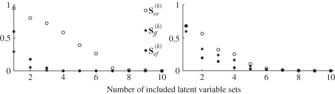
Comparing both plots in Figure 2.9 yields that MRPLS rapidly deflates ![]() . The retention of only one set of LVs produces a value below 0.3 for (2.101) and retaining a second LV set reduces this value to 0.05. In contrast, PLS deflates
. The retention of only one set of LVs produces a value below 0.3 for (2.101) and retaining a second LV set reduces this value to 0.05. In contrast, PLS deflates ![]() more rapidly than MRPLS. The retention of only three sets of LVs yields values of 0.33 and 0.72 for PLS and MRPLS, respectively. Increasing this number to six retained LV sets produces values of 0.04 and 0.28 for PLS and MRPLS, respectively. Comparing the impact of the deflation with regards to (2.104) yields a favorable performance of the MRPLS algorithm. For each number of retained LV sets, MRPLS yields a smaller value that is close to zero for i = 4. In sharp contrast, even for seven or eight sets of retained LVs, PLS does not completely deflate
more rapidly than MRPLS. The retention of only three sets of LVs yields values of 0.33 and 0.72 for PLS and MRPLS, respectively. Increasing this number to six retained LV sets produces values of 0.04 and 0.28 for PLS and MRPLS, respectively. Comparing the impact of the deflation with regards to (2.104) yields a favorable performance of the MRPLS algorithm. For each number of retained LV sets, MRPLS yields a smaller value that is close to zero for i = 4. In sharp contrast, even for seven or eight sets of retained LVs, PLS does not completely deflate ![]() .
.
On the basis of the analysis above, particularly the result presented in (2.99), however, this is expected and confirms that PLS is generally not capable of extracting common cause variation that is encapsulated in the input and output variables in an efficient manner unless the weight vectors are constrained to be orthogonal to the column space of ![]() . As this matrix is generally not known a priori, such a constraint cannot be incorporated into the PLS routine.
. As this matrix is generally not known a priori, such a constraint cannot be incorporated into the PLS routine.
2.4 Estimating the number of source signals
This section discusses the important issue of how to estimate the number of sets of latent components describing common cause variation and, accordingly, the number of source signals. This number, n, is of fundamental importance for the following reasons. If too few latent components are retained, variation that is to be attributed to the source signals is partially encapsulated in the residuals of the PCA/PLS models. On the other hand, the retention of too many latent components produces a model subspace that may capture a significant portion of the error vector(s). In the latter case, the monitoring statistics, summarized in the next chapter, describe common cause variation that is corrupted by a stronger influence of the error vector ![]() (PCA) or variation of the input variables that is not significantly predictive for the output variables, that is, en+1 or s′ for small data sets (PLS/MRPLS).
(PCA) or variation of the input variables that is not significantly predictive for the output variables, that is, en+1 or s′ for small data sets (PLS/MRPLS).
An estimation of n that is too small or too large will affect the sensitivity in detecting and diagnosing special cause variation that negatively influences product quality and/or the general state of the process operation. Hence, abnormal events may consequently not be detected nor correctly diagnosed. The question, therefore, is when to stop retaining more sets of LVs in PCA/PLS monitoring models. This question has been addressed in the literature by developing stopping rules. The stopping rules for PCA, proposed in the research literature, are summarized in Subsection 2.4.1, followed by those of PLS in Subsection 2.4.2. For the subsequent discussion of stopping rules, ![]() denotes the inclusion of
denotes the inclusion of ![]() sets of LVs that are currently being evaluated and as before, n is the selected number of sets.
sets of LVs that are currently being evaluated and as before, n is the selected number of sets.
2.4.1 Stopping rules for PCA models
The literature has introduced and discussed numerous approaches for determining how many principal components should be included, or, in relation to (2.2), how many source signals the process has. Jackson (2003) and Valle et al. (1999) provide surveys and comparisons of various stopping rules for PCA models. The aim of this subsection is to bring together the most important stopping rules, which can be divided into (i) information theoretic criterion, (ii) eigenvalue-based criterion and (iii) cross-validation-based criterion. An additional criterion that is difficult to attribute to one of these three categories is (iv) the Velicer's partial correlation procedure. These four different approaches are now separately discussed below.
2.4.1.1 Information-based criteria
These include the Akaike's Information Criterion (AIC) (Akaike 1974) and the Minimum Description Length (MDL) (Rissanen 1978; Schwarz 1978). Both criteria rely on the utilization of (2.2) under the assumption that ![]() and
and ![]() . The covariance structure of the stochastic signal component is therefore
. The covariance structure of the stochastic signal component is therefore
2.105 ![]()
with ΞSssΞT being of rank n and the discarded eigenvalues of ![]() , λn+1, λn+2, … ,
, λn+1, λn+2, … , ![]() are equal to
are equal to ![]() . The eigendecomposition of the
. The eigendecomposition of the ![]() allows a consistent estimation of
allows a consistent estimation of ![]() and
and ![]()
2.106 ![]()
Given that the eigenvectors are mutually orthonormal, the above equation reduces to
2.107 
The next step involves the utilization of the following parameter vector
2.108 ![]()
which allows the construction of the following maximum likelihood function4
2.109 
Wax and Kailath (1985) rewrote the above equation to be a log-likelihood function
where ![]() is the estimate of
is the estimate of ![]() . The maximum likelihood estimate for
. The maximum likelihood estimate for ![]() maximizes (2.110). Anderson (1963) showed that these estimates are
maximizes (2.110). Anderson (1963) showed that these estimates are
2.111 
Here, li and li are the eigenvalue and the eigenvector of ![]() . Wax and Kailath (1985) highlighted that substituting these estimates into (2.110) yields
. Wax and Kailath (1985) highlighted that substituting these estimates into (2.110) yields
2.112 
The AIC and MDL objective functions include the above term but rely on different terms to penalize model complexity. The objective functions for AIC and MDL are
2.113 
and
2.114 
respectively. Here, ![]() is the number of principal components
is the number of principal components ![]() . The selected number of principal components,
. The selected number of principal components, ![]() , is the minimum of the AIC(
, is the minimum of the AIC(![]() ) or MDL(
) or MDL(![]() ) objective functions, depending which one is used. Wax and Kailath (1985) pointed out that the MDL objective function provides a consistent estimation of n, whilst the AIC one is inconsistent and tends, asymptotically, to overestimate n.
) objective functions, depending which one is used. Wax and Kailath (1985) pointed out that the MDL objective function provides a consistent estimation of n, whilst the AIC one is inconsistent and tends, asymptotically, to overestimate n.
2.4.1.2 Eigenvalue-based criteria
Eigenvalue-based stopping rules include the cumulative percentage variance, the SCREE test, the residual percentage variance, the eigenvector-one-rule and other methods that derive from those.
Cumulative percentage variance or CPV test
This is the simplest and perhaps most intuitive eigenvalue-based test and determines the ratio of the sum of the first ![]() estimated eigenvalues over the sum of all estimated eigenvalues
estimated eigenvalues over the sum of all estimated eigenvalues
The CPV criterion relies on the fact that the sum of the squared variables of z0 is equal to the sum of squared values of the score variables. This follows from
and yields the relationship between the jth process and the nz score variables
The squared value of ![]() then becomes
then becomes
producing the following sum over the complete variable set, ![]() , ··· ,
, ··· , ![]() ,
,
2.119 
As the score variables do not include the index m, rewriting the above sum yields
2.120 
Hence, (2.118) reduces to
Finally, taking the expectation of (2.121) yields
Equation (2.122) implies that the sum of the variances of the recorded process variables is equal to the sum of the eigenvalues of the data covariance matrix. Moreover, the variance of the ith score variable is equal to the ith eigenvalue of the data covariance matrix. This is analyzed and discussed in more detail in Chapter 9.
The denominator of the CPV criterion is therefore the sum of the variances of the process variables and the numerator is the variance contribution of the retained components to this sum. Hence, the larger ![]() the closer the CPV criterion becomes to 100%. A threshold, for example 95% or 99%, can be selected and n is the number for which Equation (2.115) exceeds this threshold. Despite the simplicity of the CPV criterion, the selection of the threshold is often viewed as arbitrary and subjective, for example (Valle et al. 1999). Smaller threshold suggests including fewer components and a less accurate recovery of z0 and a larger threshold increases n. The threshold is therefore a tradeoff between parsimony and accuracy in recovering z0.
the closer the CPV criterion becomes to 100%. A threshold, for example 95% or 99%, can be selected and n is the number for which Equation (2.115) exceeds this threshold. Despite the simplicity of the CPV criterion, the selection of the threshold is often viewed as arbitrary and subjective, for example (Valle et al. 1999). Smaller threshold suggests including fewer components and a less accurate recovery of z0 and a larger threshold increases n. The threshold is therefore a tradeoff between parsimony and accuracy in recovering z0.
SCREE test
This test plots the eigenvalues of the ![]() against their number in descending order, which is referred to as a SCREE plot. Cattell (1966) highlighted that SCREE plots often show that the first few eigenvalues decrease sharply in value whilst most of the remaining ones align along a line that slowly decreases and further suggested to retain the first few sharply decreasing eigenvalues and the first one of the second set of slowly decreasing eigenvalues. If more than one such elbow emerges, Jackson (2003) pointed out that the first of these breaks determines the number of retained principal components. Conditions under which a larger number of principal components should be retained if the SCREE plot produces multiple elbows are discussed in Box et al. (1973); Cattell and Vogelmann (1977).
against their number in descending order, which is referred to as a SCREE plot. Cattell (1966) highlighted that SCREE plots often show that the first few eigenvalues decrease sharply in value whilst most of the remaining ones align along a line that slowly decreases and further suggested to retain the first few sharply decreasing eigenvalues and the first one of the second set of slowly decreasing eigenvalues. If more than one such elbow emerges, Jackson (2003) pointed out that the first of these breaks determines the number of retained principal components. Conditions under which a larger number of principal components should be retained if the SCREE plot produces multiple elbows are discussed in Box et al. (1973); Cattell and Vogelmann (1977).
Residual percentage variance or RPV test
Similar to the CPV test, the RPV test determines n from the last few eigenvalues (Cattell 1966; Rozett and Petersen 1975)
2.123 
Average-eigenvalue test
Kaiser (1960) proposed an extension of the SCREE test that relies on the property that the trace of the covariance/correlation matrix is equal to the sum of the eigenvalues, which follows from the relationship in (2.117) to (2.122). Using (2.122), the average eigenvalue, ![]() , can be directly calculated from the trace of the data covariance/correlation matrix
, can be directly calculated from the trace of the data covariance/correlation matrix
2.124 ![]()
This rule suggests that eigenvalues that are larger or equal to ![]() should be associates with the source signals and those below
should be associates with the source signals and those below ![]() corresponding to the error vector. If
corresponding to the error vector. If ![]() is used instead of
is used instead of ![]() the average eigenvalue is 1, as all of the diagonal elements are 1. With the use of
the average eigenvalue is 1, as all of the diagonal elements are 1. With the use of ![]() this rule is referred to as the eigenvalue-one-rule.
this rule is referred to as the eigenvalue-one-rule.
Alternative methods
Jolliffe (1972, 1973) conducted a critical review of the average-eigenvalue rule and concluded that the threshold for selecting the number of retained components may be too high. Based on a number of simulation examples, a recommendation in these references was to discard components that correspond to eigenvalues up 70% of the average eigenvalue.
To automate the SCREE test, Horn (1965) proposed the utilization of a second data set that includes the same number of samples and variables. This second data set, however, should include statistically uncorrelated Gaussian variables, so that the covariance matrix reduces to a diagonal matrix. The eigenvalues of both covariance matrices are then plotted in a single SCREE plot where the interception determines the cutoff point for separating retained from discarded components.
The use of the correlation matrix, that is, the identify matrix, reduces this method to the eigenvalue-one-rule. Farmer (1971) proposed a similar approach to that in (Horn 1965) using logarithmic SCREE plots. Procedures that rely on the incorporation of a second artificially generated data set are also referred to as parallel analysis. Other techniques that utilize the eigenvalues include the indicator function, the embedded error function (Malinowski 1977) and the broken stick model (Jolliffe 1986).
2.4.1.3 Cross-validation-based criteria
Cross-validation relies on the residuals ![]() and was first proposed by Mosteller and Wallace (1963) and further discussed in Allen (1974) and Stone (1974) among others. The main principle behind cross-validation is:
and was first proposed by Mosteller and Wallace (1963) and further discussed in Allen (1974) and Stone (1974) among others. The main principle behind cross-validation is:
Figure 2.10 illustrates the structured cross-validation approach, which segments the reference data set equally into groups. The first group is used to test the PCA model constructed from the remaining groups, then the second group is used etc.
Figure 2.10 Schematic representation of a structured cross-validation approach.
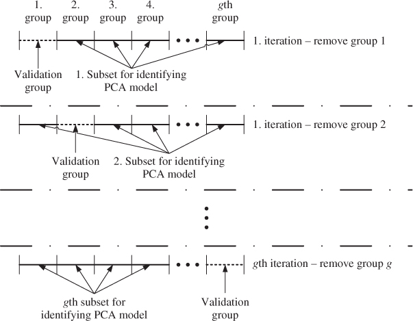
Stone (1974) argued on theoretical grounds that the number of groups should be equal to the number of observations, which leads to an excessive computation. Geisser (1974) showed that using fewer groups is sufficient. This view is also echoed in Wold (1978). The research literature has proposed a number of performance indices, including the R and W statistics. A different cross-validation approach that omits variables rather than observations was proposed in Qin and Dunia (2000).
Cross-validation based on the R statistic
For the ith group, Wold (1978) suggested using the ratio of the PRESS statistic (PREdiction Sum of Squares) over the RSS statistic (Residual Sum of Squares)
2.125 ![]()
where
2.126 
and
2.127 
with ![]() being the number of samples in the ith group. The sum over the g groups is
being the number of samples in the ith group. The sum over the g groups is
2.128 ![]()
If ![]() is below one then increase
is below one then increase ![]() to
to ![]() , since the inclusion of the
, since the inclusion of the ![]() th component increases the prediction accuracy relative to the (
th component increases the prediction accuracy relative to the (![]() )th one. In contrast, if
)th one. In contrast, if ![]() exceeds one than this new component does not reduce the prediction accuracy. This stopping rule is often referred to as the R ratio or R statistic and the number of source signals is equal to the first n R ratios below one, that is, R(1), … , R(n) < 1.
exceeds one than this new component does not reduce the prediction accuracy. This stopping rule is often referred to as the R ratio or R statistic and the number of source signals is equal to the first n R ratios below one, that is, R(1), … , R(n) < 1.
Cross-validation based on the W statistic
Eastment and Krzanowski (1982) proposed an alternative criterion, defined as the W statistic, that involves the PRESS statistics for PCA models that include ![]() and
and ![]() retained components
retained components
2.129 ![]()
where Dr and ![]() are the number of degrees of freedom that remain after determining the
are the number of degrees of freedom that remain after determining the ![]() th component and for constructing the
th component and for constructing the ![]() th component, respectively,
th component, respectively,
2.130 
Components that have a ![]() value larger than 1 should be included in the PCA model. Eastment and Krzanowski (1982) suggested that the optimum number of source signals is the last one for which
value larger than 1 should be included in the PCA model. Eastment and Krzanowski (1982) suggested that the optimum number of source signals is the last one for which ![]() . A discussion of these cross-validatory stopping rules in Wold et al. (1987), highlighted that they work well and the use of a proper algorithm does not render them too computationally expensive and concluded that cross-validation is slightly conservative yielding too few rather than too many components. The discussion, however, deemed this as an advantage as it circumvents an over-interpretation of the encapsulated information.
. A discussion of these cross-validatory stopping rules in Wold et al. (1987), highlighted that they work well and the use of a proper algorithm does not render them too computationally expensive and concluded that cross-validation is slightly conservative yielding too few rather than too many components. The discussion, however, deemed this as an advantage as it circumvents an over-interpretation of the encapsulated information.
Variance of the reconstruction error (VRE)
A different approach to those by Wold (1978) and Eastment and Krzanowski (1982) is discussed in Qin and Dunia (2000). Instead of leaving portions of the reference data out, this technique omits the samples of one variable and reconstructs it by the remaining nz − 1 ones. Evaluating the accuracy of this reconstruction by PCA models for different numbers of source signals, each variable is removed and reconstructed by the remaining ones. This produces a total of nz contributions to the VRE performance index.
Using the eigendecomposition ![]() and defining
and defining ![]() , the projection of z0 onto the model subspace
, the projection of z0 onto the model subspace ![]() is for the ith element
is for the ith element
2.131 
where ![]() is the element of
is the element of ![]() stored in the ith row and the jth column. Replacing the variable
stored in the ith row and the jth column. Replacing the variable ![]() by
by ![]() the above equation becomes
the above equation becomes
2.132 
The reconstruction of ![]() ,
, ![]() , is therefore
, is therefore
A more detailed treatment of variable reconstruction is given in Section 3.2. Equation (2.133) outlines that the number of retained components can vary from 1 to nz − 1. For ![]() ,
, ![]() and the denominator becomes zero. The use of (2.133) gives rise to the following reconstruction error
and the denominator becomes zero. The use of (2.133) gives rise to the following reconstruction error
Next, abbreviating ![]() and rewriting (2.134) yields
and rewriting (2.134) yields
Noting that ![]() is equal to the ith row or column of the symmetric matrix
is equal to the ith row or column of the symmetric matrix ![]() , this vector is also equal to
, this vector is also equal to
2.136 ![]()
where ![]() is the ith Euclidean vector whose ith element is 1, whilst any other element is 0. Equation (2.135) can therefore be expressed as follows
is the ith Euclidean vector whose ith element is 1, whilst any other element is 0. Equation (2.135) can therefore be expressed as follows
2.137 
Expressing ![]() as a function of
as a function of ![]() and
and ![]()
2.138 
the variance of the reconstruction error for the ith variable becomes
2.139 
Since ![]() , the above equation reduces to
, the above equation reduces to
2.140 
Finally, defining ![]() , the VRE criteria is given by
, the VRE criteria is given by

where ![]() is the variance of the ith process variable. Valle et al. (1999) pointed out that the scaling of the reconstruction error is necessary, as variables that have a larger variance produce, by default, larger reconstruction errors and may have a dominant influence upon the calculation of the VRE performance index. The value of
is the variance of the ith process variable. Valle et al. (1999) pointed out that the scaling of the reconstruction error is necessary, as variables that have a larger variance produce, by default, larger reconstruction errors and may have a dominant influence upon the calculation of the VRE performance index. The value of ![]() that yields a minimum for the VRE performance index is then n.
that yields a minimum for the VRE performance index is then n.
A detailed discussion in Qin and Dunia (2000) showed that (2.141) yields a minimum, which is related to the fact that, according to (2.2), the data space is separated into a model subspace and a complementary residual subspace. Moreover, Valle et al. (1999) (i) proved that the VRE approach gives a consistent estimation of the number of source signals under the assumptions that the error vector ![]() (i) contains Gaussian i.i.d. sequences and (ii) postulated that it also gives a consistent estimation of the number of source signals if the error vector contains Gaussian sequences that have slightly different variances.
(i) contains Gaussian i.i.d. sequences and (ii) postulated that it also gives a consistent estimation of the number of source signals if the error vector contains Gaussian sequences that have slightly different variances.
Valle et al. (1999) argued that the VRE method is to be preferred over cross-validatory methods for consistently estimating the number of source signals and in terms of computational costs. By directly comparing various stopping rules, including VRE, AIC, MDL, CPV, RPV and cross-validation based on the R-statistics, Valle et al. (1999) showed that the VRE method performed favorably. Despite the conceptual ease and computational efficiency of the VRE stopping rule, however, Subsection 6.1.1 shows that the above postulate, differences in the error variances, may not yield a consistent estimate for n, which is also demonstrated in Feital et al. (2010).
2.4.1.4 Velicer's Partial Correlation Criterion (VPC)
Velicer (1976) proposed this technique, which carries out a scaled deflation of the covariance matrix each time ![]() is increased by 1. Starting with the deflation of the covariance matrix
is increased by 1. Starting with the deflation of the covariance matrix
2.142 ![]()
the scaling process for ![]() involves the diagonal matrix
involves the diagonal matrix ![]()
2.143 ![]()
where
2.144 
and ![]() ,
, ![]() , ··· ,
, ··· , ![]() are the diagonal elements of
are the diagonal elements of ![]() . The VPC criterion relies on the sum of the non-diagonal elements of
. The VPC criterion relies on the sum of the non-diagonal elements of ![]()
2.145 
In fact, ![]() is a correlation matrix. Hence,
is a correlation matrix. Hence, ![]() are correlation coefficients for i ≠ j and the VPC performance index is larger than zero within the range of
are correlation coefficients for i ≠ j and the VPC performance index is larger than zero within the range of ![]() and
and ![]() . The estimation of n is given by the minimum of VPC
. The estimation of n is given by the minimum of VPC![]() . The underlying assumption for the VPC method is that the VPC curve decreases in value for an additional source variable if the average remaining covariance reduces faster than the remaining variance of the variable set. In contrast, an increase indicates that an additional source signal explains more variance than covariance.
. The underlying assumption for the VPC method is that the VPC curve decreases in value for an additional source variable if the average remaining covariance reduces faster than the remaining variance of the variable set. In contrast, an increase indicates that an additional source signal explains more variance than covariance.
2.4.2 Stopping rules for PLS models
The literature has proposed a number of different stopping rules, which include:
- analysis of variance approaches;
- cross validation criteria based on the accuracy of the PLS model in predicting the output variables;
- bootstrapping criteria; and
- the H-principle.
These different methods are now discussed separately.
2.4.2.1 Analysis of variance criteria
An analysis of variance can be carried out for the u-score or output variables (Jackson 2003). More practical and intuitive, however, is the use of the residuals of y0. In a similar fashion to the SCREE test for PCA, the Frobenius norm of the residual matrix
2.146 ![]()
can be plotted vs. ![]() . The norm
. The norm ![]() often shows an initial sharp decrease when retaining the first few sets of LVs and then slowly decays as additional sets are included. Like a SCREE plot, n can be estimated from the intercept between a tangent that represents the first (few) sharp decrease(s) and a parallel line to the abscissa of value,
often shows an initial sharp decrease when retaining the first few sets of LVs and then slowly decays as additional sets are included. Like a SCREE plot, n can be estimated from the intercept between a tangent that represents the first (few) sharp decrease(s) and a parallel line to the abscissa of value, ![]() . Section 2.2 presents an example of using
. Section 2.2 presents an example of using ![]() to determine the number of source signals (Table 2.2). This example, however, divides
to determine the number of source signals (Table 2.2). This example, however, divides ![]() by ||Y0||2 and uses a percentage figure.
by ||Y0||2 and uses a percentage figure.
2.4.2.2 Cross-validation criterion
Lindberg et al. (1983) proposed a cross-validatory stopping rule that relies on the principle outlined in Figure 2.10. Segmenting the reference data into g groups, each group is once omitted for the identification of a PLS model. The prediction of the output variables is then assessed on the basis of the group that is left out. The performance index for the gth group is the PRESS statistic
for which
2.148 ![]()
Including each of the G groups, the PRESS statistic finally becomes
2.149 
If minimum of the resulting curve for ![]() exists, then this is the selected number of source signals. If this curve. however, decreases monotonically without showing a clear minimum n can be selected by the intercepting the tangent that describes the first (few) steep decrease(s) and the parallel line to the abscissa. Published work on cross-validation include Qin (1998) and Rännar et al. (1995). The latter work, however, discusses cases where there are considerably more variables than samples.
exists, then this is the selected number of source signals. If this curve. however, decreases monotonically without showing a clear minimum n can be selected by the intercepting the tangent that describes the first (few) steep decrease(s) and the parallel line to the abscissa. Published work on cross-validation include Qin (1998) and Rännar et al. (1995). The latter work, however, discusses cases where there are considerably more variables than samples.
2.4.2.3 Bootstrapping criterion
As the analysis of variance relies on the user to select n and cross-validation may be computationally expensive, bootstrapping can be proposed as an alternative. Bootstrapping, in this context, relates to recent work on entropy-based independence tests (Dionisio and Mendes 2006; Wu et al. 2009), which tests the hypothesis that two variables are independent. Scaling the ![]() th pair of score variables to unit variance, that is,
th pair of score variables to unit variance, that is, ![]() and
and ![]() , the corresponding hypothesis is as follows
, the corresponding hypothesis is as follows
2.150 ![]()
The above hypothesis can alternatively be expressed as
Here, ![]() ,
, ![]() ,
, ![]() and
and ![]() are the
are the ![]() th p-weight and q-loading vectors, respectively, and
th p-weight and q-loading vectors, respectively, and ![]() is the covariance of
is the covariance of ![]() and
and ![]() . Chapter 10 provides a description of PLS including the relationship used in (2.151).
. Chapter 10 provides a description of PLS including the relationship used in (2.151).
To test the null hypothesis, Granger et al. (2004) proposed the following procedure. Defining two independent Gaussian distributed white noise sequences of zero mean and variance 1, θ and ϕ, the critical value for testing the null hypothesis can be obtained from a smoothed bootstrap procedure (Efron and Tibshirani 1993) for the upper α-percentile using ![]() samples of θ and ϕ, with K being the number of elements of
samples of θ and ϕ, with K being the number of elements of ![]() and
and ![]() .
.
![]()
The null hypothesis, H0, is accepted if
and rejected if ![]() . In (2.152),
. In (2.152), ![]() ,
, ![]() , where
, where ![]() is the variance of the
is the variance of the ![]() th t-score variable. Moreover,
th t-score variable. Moreover, ![]() and
and ![]() . The computation of
. The computation of ![]() and
and ![]() follows from the deflation procedure that is discussed and analyzed in Chapter 10.
follows from the deflation procedure that is discussed and analyzed in Chapter 10.
It should be noted that rejection of H0 results in accepting H1, which implies that the ![]() th pair of latent variables need to be included in the PLS model and requires the calculation of the
th pair of latent variables need to be included in the PLS model and requires the calculation of the ![]() th pair of latent variables after carrying out the deflation procedure. On the other hand, accepting the null hypothesis sets
th pair of latent variables after carrying out the deflation procedure. On the other hand, accepting the null hypothesis sets ![]() .
.
Table 2.4 lists estimated confidence limits for significance levels of:
- α = 5%, 1%, 0.5%, 0.1%, 0.05% and 0.01%
and different sample sizes:
- K = 100, 200, 500, 1000, 2000, 5000 and 10000.
Table 2.4 Confidence limits for various sample sizes, K and significance levels α.
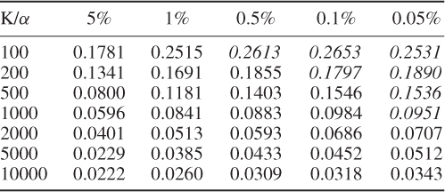
The entries in Table 2.4 are averaged values over a total of 10 runs for each combination of sample size and significance level. For a reference set containing 5000 samples, for example, the confidence limit for the smoothed bootstrap approach was selected to be α = 0.5%, i.e. 0.0433.
2.4.2.4 H-Principle
Finally, Höskuldsson (1994) showed an alternative approach for deriving the PCA and PLS objective functions, which is inspired by the Heisenberg uncertainty inequality and referred to as the H-principle. This objective function is a product of a goodness of fit and a precision criterion. More precisely, Höskuldsson (1994, 1995, 2008) showed that the PCA and PLS objective functions can be derived from the H-principle including an estimation of n. A more detailed discussion regarding the H-principle, however, is beyond the scope of this book.
2.5 Tutorial Session
Question 1:
Compare the maximum number of sets of LVs that can be obtained by applying the PLS, the maximum redundancy and the CCA (Chapter 10) objective function if the covariance and cross-covariance matrices are known and of arbitrary dimension. Why can PLS exhaust the input variable set irrespective of the number of input and output variables, whilst maximum redundancy and CCA cannot?
Question 2:
Following from Question 1, why does MSPC rely on the use of variance and covariance-based methods, i.e. PCA and PLS, for providing a data model for the recorded variable set(s)?
Question 3:
Assuming that z0 = x0, why can PCA and PLS be seen as unsupervised and supervised learning algorithms, respectively?
Question 4:
Why is it beneficial to rely on statistically independent score variables, which PCA and PLS extract from the data and input variable set, respectively, instead of the original variable sets?
Question 5:
Explain the difference between the PLS and MRPLS objective function. What do the extracted score variables explain in both cases?
Project 1:
With respect to the simulation example in Subsection 2.1.3, use a Monte-Carlo simulation and vary the number of reference samples, and analyze this impact on the accuracy of estimating the data covariance matrix and its eigendecomposition.
Project 2:
Carry out a Monte-Carlo simulation to estimate the elements of the regression matrix (simulation example in Subsection 2.2.3) by varying the number of reference samples and the number of retained sets of LVs and comment upon your findings. Contrast your results with the simulation example in Subsection 6.2.2.
Project 3:
Develop a deflation-based method for CCA to extract the common cause variation encapsulated in the input and output variables with respect to the data structure in (2.51). Use the simulation example in Subsection 2.3.4 and compare the performance of the developed CCA method with that of MRPLS with particular focus on the predictability of the output variables.
Project 4:
Generate a data model with respect to (2.2) that includes a total of nz = 20 process variables, a varying number of source signals 1 ≤ n < 19, a varying error variance ![]() , a varying number of reference samples K and apply each of the stopping rules in Section 2.4.1 to estimate n. Comment and explain the results. Which method is most successful in correctly estimating n?
, a varying number of reference samples K and apply each of the stopping rules in Section 2.4.1 to estimate n. Comment and explain the results. Which method is most successful in correctly estimating n?
1 The variable s describes the distance between the projection of the sample ![]() onto the semimajor from the origin of the control ellipse which, according to Figure 1, is given by the interception the abscissas of both Shewhart charts.
onto the semimajor from the origin of the control ellipse which, according to Figure 1, is given by the interception the abscissas of both Shewhart charts.
2 The assumptions for this are discussed in Subsection 6.1.1.
3 A dominant eigenvector is the eigenvector associated with the largest eigenvalue of a symmetric positive semi-definite matrix under the assumption that this eigenvalue is not a multiple eigenvalue of that matrix.
4 Information about parameter estimation using maximum likelihood is given in Subsection 6.1.3.