
Chapter 3
Process monitoring charts
The aim of this chapter is:
- to design monitoring charts on the basis of the extracted LV sets and the residuals;
- to show how to utilize these charts for evaluating the performance of the process and for assessing product quality on-line; and
- to outline how to diagnose behavior that is identified as abnormal by these monitoring charts.
For monitoring a complex process on-line, the set of score and residual variables give rise to the construction of a statistical fingerprint of the process. This fingerprint serves as a benchmark for assessing whether the process is in-statistical control or out-of-statistical-control. Based on Chapters 3 and Chapters 2, the construction of this fingerprint relies on the following assumptions for identifying PCA/PLS data models:
- the error vectors associated with the PCA/PLS data models follow a zero mean Gaussian distribution that is described by full rank covariance matrices;
- the score variables, describing common cause variation of the process, follow a zero mean Gaussian distribution that is described by a full rank covariance matrix;
- for any recorded process variable, the variance contribution of the source signals (common cause variation) is significantly larger than the variance contribution of the corresponding error signal;
- the number of source variables is smaller than the number of recorded process (PCA) or input variables (PLS);
- recorded variable sets have constant mean and covariance matrices over time;
- the process is a representation of the data models in either 2.2, 2.24 or 2.51;
- none of the process variables possess any autocorrelation; and
- the cross-correlation function of any pair of process variables is zero for two different instances of time, as described in Subsection 2.1.1.
Part III of this book presents extensions of conventional MSPC which allow relaxing the above assumptions, particularly the assumption of Gaussian distributed source signals and time-invariant (steady state) process behavior.
The statistical fingerprint includes scatter diagrams, which Section 1.2 briefly touched upon, and non-negative squared statistics involving the t-score variables and the residuals of the PCA and PLS models. For the construction of monitoring models, this chapter assumes the availability of the data covariance and cross-covariance matrices. In this regard, the weight, loading and score variables do not need to be estimated from a reference data set. This simplifies the presentation of the equations derived, as the hat notation is not required.
Section 3.1 introduces the tools for constructing the statistical fingerprint for on-line process monitoring and detecting abnormal process conditions that are indicative of a fault condition. Fault conditions could range from simple sensor or actuator faults to complex process faults. Section 3.2 then summarizes tools for diagnosing abnormal conditions to assist experienced plant personnel in narrowing down potential root causes. Such causes could include, among many other possible scenarios, open bypass lines, a deteriorating performance of a heat exchanger, a tray or a pump, a pressure drop in a feed stream, a change in the input composition of input feeds, abnormal variation in the temperature of input or feed streams, deterioration of a catalyst, partial of complete blockage of pipes and valve stiction.
The diagnosis offered in Section 3.2 identifies to what extent a recorded variable is affected by an abnormal event. This section also shows how to extract time-based signatures for process variables if the effect of a fault condition deteriorates the performance of the process over time. Section 3.3 finally presents (i) a geometric analysis of the PCA and PLS projections to demonstrate that fault diagnosis based on the projection of a single sample along predefined directions may lead to erroneous and incorrect diagnosis results in the presence of complex fault conditions and (ii) discusses how to overcome this issue. A tutorial session concerning the material covered in this chapter is given in Section 3.4.
3.1 Fault detection
Following from the discussion in Chapter 2, PCA and PLS extract latent information in form of latent score variables and residuals from the recorded variables. According to the data models for PCA in 2.2 and 2.6 and PLS in 2.23, 2.24 and 2.51, the t-score variables describe common cause variation that is introduced by the source vector s. Given that the number of t-score variables is typically significantly smaller than the number of recorded variables, MSPC allows process monitoring on the basis of a reduced set of score variables rather than relying on charting a larger number of recorded process variables.
With respect to the assumptions made for the data structures for PCA and PLS in Chapter 2, the variation described by the t-score variables recovers the variation of the source variables. Hence, the variation encapsulated in the t-score variables recovers significant information from recorded variables, whilst the elements in the error vector have an insignificant variance contribution to the process variable set. Another fundamental advantage of the t-score variables is that they are statistically independent, which follows from the analysis of PCA and PLS in Chapters 9 and 10, respectively.
The t-score variables can be plotted in scatter diagrams for which the confidence regions are the control ellipses discussed in Subsection 1.2.3. For a time-based analysis, MSPC relies on nonnegative quadratics that includes Hotelling's T2 statistics and residual-based squared prediction error statistics, referred to here as Q statistics. Scatter diagrams are not time-based but allow the monitoring of pairs or triples of combinations of t-score variables. In contrast, the time-based Hotelling's T2 statistics present an overall measure of the variation within the process.
The next two subsections provide a detailed discussion of scatter diagrams and the Hotelling's T2 statistic. It is important to note that MRPLS may generate two Hotelling's T2 statistics, one for the common cause variation in the predictor and response variable sets and one for variation that is only manifested in the input variables and is not predictive for the output variables. This is discussed in more detail in the next paragraph and Subsection 3.1.2.
The mismatch between the recorded variables and what the t-score variables, or source variables, can recover from the original variables are model residuals. Depending on the variance of the discarded t-score variables (PLS) or the variance of the t′-scores (MRPLS), these score variables may be used to construct a Hotelling's T2 or a residual Q statistic. Whilst Hotelling's T2 statistics present a measure that relates to the source signals, or significant variation to recover the input variables, the residual Q statistic is a measure that relates to the model residuals.
Loosely speaking, a Q statistic is a measure of how well the reduced dimensional data representation in 2.2, 2.24 or 2.51 describe the recorded data. Figure 1.7 presents an illustration of perfect correlation, where the sample projections fall onto the line describing the relationship between both variables. In this extreme case, the residual vector is of course zero, as the values of both variables can be recovered without an error from the projection of the associated sample.
If, however, the projection of a sequence of samples do not fall onto this line an error for the recovery of the original variables has occurred, which is indicative of abnormal process behavior. For a high degree of correlation, Figure 1.9 shows that the recovered values of each sample using the projection of the samples onto the semimajor of the control ellipse are close to the recorded values. The perception of ‘close’ can be statistically described by the residual variables, its variances and the control limit of the residual based monitoring statistic.
3.1.1 Scatter diagrams
Figures 1.6, Figures 1.7 and 1.9 show that the shape of the scatter diagrams relate to the correlation between two variables. Different from the 2D scatter diagrams, extensions to 3D scatter diagrams are possible, although it is difficult to graphically display a 3D control sphere. For PCA and PLS, the t-score variables, ![]() for PCA and
for PCA and ![]() for PLS are uncorrelated and have the following covariance matrices
for PLS are uncorrelated and have the following covariance matrices
and
The construction of the weight matrix R is shown in Chapter 10. Under the assumption that the exact data covariance matrix is known a priori, the control ellipse for i ≠ j has the following mathematical description
where ![]() is the critical value of a χ2 distribution with two degrees of freedom and a significance of α. The length of both axes depends on the variance of the ith and jth t-score variable, denoted by
is the critical value of a χ2 distribution with two degrees of freedom and a significance of α. The length of both axes depends on the variance of the ith and jth t-score variable, denoted by ![]() and
and ![]() for PCA, and
for PCA, and ![]() and
and ![]() for PLS. These variances correspond to the diagonal elements of the matrices in (3.1) and (3.2), noting that 1 ≤ i, j ≤ n.
for PLS. These variances correspond to the diagonal elements of the matrices in (3.1) and (3.2), noting that 1 ≤ i, j ≤ n.
It is straightforward to generate a control ellipse for any combination of score variables for n > 2. This, however, raises the following question: how can such scatter plots be adequately depicted? A naive solution would be to extend the 2D concept into an nD concept, where the 2D control ellipse becomes an nD-ellipsoid
where ![]() is the critical value of a χ2 distribution with n degrees of freedom. While it is still possible to depict a control ellipsoid that encompasses the orthogonal projections of the data points onto the n = 3-dimensional model subspace, however, this is not the case for n > 3. A pragmatic solution could be to display pairs of score variables, an example of which is given in Chapter 5.
is the critical value of a χ2 distribution with n degrees of freedom. While it is still possible to depict a control ellipsoid that encompasses the orthogonal projections of the data points onto the n = 3-dimensional model subspace, however, this is not the case for n > 3. A pragmatic solution could be to display pairs of score variables, an example of which is given in Chapter 5.
It is important to note that (3.3) and (3.4) only hold true if the exact covariance matrix of the recorded process variables is known (Tracey et al. 1992). If the covariance matrix must be estimated from the reference data, as shown in Sections 2.1 and 2.2, the approximation by a χ2-distribution may be inaccurate if few reference samples, K, are available. In this practically important case, (3.4) follows an F-distribution under the assumption that the covariance matrix of the score variables has been estimated independently from the score variables. For a detailed discussion of this, refer to Theorem 5.2.2. in Anderson (2003). The critical value ![]() in this case is given by (MacGregor and Kourti 1995; Tracey et al. 1992)
in this case is given by (MacGregor and Kourti 1995; Tracey et al. 1992)
where ![]() is the critical value of an F-distribution for n and K − n degrees of freedom, and a significance of α. It should be noted that the value of
is the critical value of an F-distribution for n and K − n degrees of freedom, and a significance of α. It should be noted that the value of ![]() converges to
converges to ![]() as K → ∞ (Tracey et al. 1992) and if the variable mean is known a priori,
as K → ∞ (Tracey et al. 1992) and if the variable mean is known a priori, ![]() becomes (Jackson 1980)
becomes (Jackson 1980)
3.1.2 Non-negative quadratic monitoring statistics
Non-negative quadratic statistics could be interpreted as a kinetic energy measure that condenses the variation of a set of n score variables or the model residuals into single values. The reference to non-negative quadratics was proposed by Box (1954) and implies that it relies on the sum of squared values of a given set of stochastic variables. For PCA, the t-score variables and the residual variables can be used for such statistics. In the case of PLS, however, a total of three univariate statistics can be established, one that relates to the t-score variables and two further that correspond to the residuals of the output and the remaining variation of the input variables.
The next two paragraphs present the definition of non-negative quadratics for the t-score variables and detail the construction of the residual-based ones for PCA and PLS. For the reminder of this book, the loading matrix for PCA and PLS are denoted as P and only contain the first n column vectors, that is, the ones referring to common-cause variation. For PCA and PLS, this matrix has nz and n, and nx and n columns and rows, respectively. The discarded loading vectors are stored in a second matrix, defined as Pd. Moreover, the computed score vector, ![]() for PCA and
for PCA and ![]() for PLS is of dimension n.
for PLS is of dimension n.
3.1.2.1 PCA monitoring models
The PCA data model includes the estimation of:
- the model subspace;
- the residual subspace;
- the error covariance matrix;
- the variance of the orthogonal projection of the samples onto the loading vectors; and
- the control ellipse/ellipsoid.
The model and residual subspaces are spanned by the column vectors of P and Pd, respectively. Sections 6.1 and 9.1 provide a detailed analysis of PCA, where these geometric aspects are analyzed in more detail.
According to 2.2, the number of source signals determines the dimension of the model subspace. The projection of the samples onto the model subspace therefore yields the source variables that are corrupted by the error variables, which the relationship in 2.8 shows. Moreover, the mismatch between the data vector z0 and the orthogonal projection of z0 onto the model subspace, g, does not include any information of the source signals, which follows from
3.7 
The above relationship relies on the fact that ![]() , which 2.7 outlines, and the eigenvectors of the data covariance matrix are mutually orthonormal. The score vector
, which 2.7 outlines, and the eigenvectors of the data covariance matrix are mutually orthonormal. The score vector ![]() , approximating the variation of the source vector s, and the residual vector g give rise to the construction of two non-negative squared monitoring statistics, the Hotelling's T2 and Q statistics that are introduced below.
, approximating the variation of the source vector s, and the residual vector g give rise to the construction of two non-negative squared monitoring statistics, the Hotelling's T2 and Q statistics that are introduced below.
Hotelling's T2 statistic
The univariate statistic for the t-score variables, ![]() is defined as follows
is defined as follows
3.8 ![]()
The matrix Λ includes the largest n eigenvalues of ![]() as diagonal elements. For a significance α, the control limit for the above statistic,
as diagonal elements. For a significance α, the control limit for the above statistic, ![]() is equal to χ2(n) if the covariance matrix of the recorded process variables is known. If this is not the case the control limit can be obtained as shown in (3.5) or (3.6). The above non-negative quadratic is also referred to as a Hotelling's T2 statistic. The null hypothesis for testing whether the process is in-statistical-control, H0, is as follows
is equal to χ2(n) if the covariance matrix of the recorded process variables is known. If this is not the case the control limit can be obtained as shown in (3.5) or (3.6). The above non-negative quadratic is also referred to as a Hotelling's T2 statistic. The null hypothesis for testing whether the process is in-statistical-control, H0, is as follows
3.9 ![]()
and the hypothesis H0 is rejected if
3.10 ![]()
The alternative hypothesis H1, the process is out-of-statistical-control, is accepted if H0 is rejected.
Assuming that the fault condition, representing the alternative hypothesis H1, describes a bias of the mth sensors, denoted by zf = z0 + Δz where the mth element of Δz is nonzero and the remaining entries are zeros, the score variables become ![]() . This yields the following impact upon the Hotelling's T2 statistic, denoted here by
. This yields the following impact upon the Hotelling's T2 statistic, denoted here by ![]() where the subscript f refer to the fault condition
where the subscript f refer to the fault condition
The above equation uses ![]() . The alternative hypothesis, H1, is therefore accepted if
. The alternative hypothesis, H1, is therefore accepted if
3.12 ![]()
and rejected if ![]() . A more detailed analysis of the individual terms in (3.11)
. A more detailed analysis of the individual terms in (3.11) ![]() ,
, ![]() and
and ![]() yields that
yields that
 ;
; ;
; ;
; ; and
; and .
.
If the term ![]() is hypothetically set to zero,
is hypothetically set to zero, ![]() . The larger the fault magnitude, Δzm the more the original T2 statistic is shifted, which follows from
. The larger the fault magnitude, Δzm the more the original T2 statistic is shifted, which follows from
3.13 
which is equal to
3.14 ![]()
The impact of the term ![]() upon
upon ![]() is interesting since it represents a Gaussian distributed contribution. This, in turn, implies that the PDF describing
is interesting since it represents a Gaussian distributed contribution. This, in turn, implies that the PDF describing ![]() is not only a shift of T2 by
is not only a shift of T2 by ![]() but it has also a different shape.
but it has also a different shape.
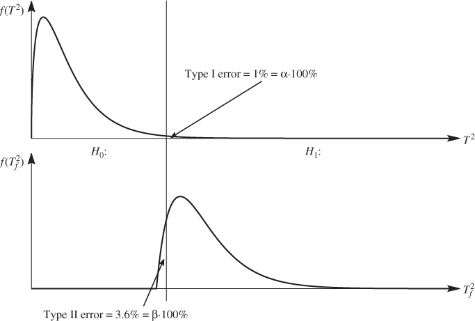
Figure 3.1 presents the PDFs that describe the T2 and ![]() and illustrate the impact of Type I and II errors for the hypothesis testing. It follows from Subsections 1.1.3 and 1.2.4 that a Type I error is a rejecting of the null hypothesis although it is true and a Type II error is the acceptance of the null hypothesis although it is false. Figure 3.1 shows that the significance level for the Type II, β, depends on the exact PDF for a fault condition, which, even the simple sensor fault, is difficult to determine. The preceding discussion, however, highlights that the larger the magnitude of the fault condition the more the PDF will be shifted and hence, the smaller β becomes. In other words, incipient fault conditions are more difficult to detect than faults that have a profound impact upon the process.
and illustrate the impact of Type I and II errors for the hypothesis testing. It follows from Subsections 1.1.3 and 1.2.4 that a Type I error is a rejecting of the null hypothesis although it is true and a Type II error is the acceptance of the null hypothesis although it is false. Figure 3.1 shows that the significance level for the Type II, β, depends on the exact PDF for a fault condition, which, even the simple sensor fault, is difficult to determine. The preceding discussion, however, highlights that the larger the magnitude of the fault condition the more the PDF will be shifted and hence, the smaller β becomes. In other words, incipient fault conditions are more difficult to detect than faults that have a profound impact upon the process.
Figure 3.1 Illustration of Type I and II errors for testing null hypothesis.
Q statistic
The second non-negative quadratic statistic relates to the PCA model residuals ![]() and is given by
and is given by
The control limit for the Q statistic is difficult to obtain although the above sum appears to be the sum of squared values. More precisely, Subsection 3.3.1 highlights that the PCA residuals are linearly dependent and are therefore not statistically independent. Approximate distributions for such quadratic forms were derived in Box (1954) and Jackson and Mudholkar (1979). Appendix B in Nomikos and MacGregor (1995) yielded that both approximations are close. Using the method by Jackson and Mudholkar (1979) the control limit for the Q statistic is as follows

where ![]() ,
, ![]() ,
, ![]() ,
, ![]() and the variable cα is the normal deviate evaluated for the significance α. Defining the matrix product
and the variable cα is the normal deviate evaluated for the significance α. Defining the matrix product ![]() , (3.15) can be rewritten as follows
, (3.15) can be rewritten as follows
where ![]() is the element of
is the element of ![]() stored in the jth row and the ith column. Given that
stored in the jth row and the ith column. Given that ![]() is symmetric, i.e.
is symmetric, i.e. ![]() , (3.17) becomes
, (3.17) becomes
3.18 
A modified version of the Q statistic in (3.15) was proposed in (Hawkins 1974) and entails a scaling of each discarded score vector by its variance
3.19 ![]()
and follows a χ2 distribution with the control limit ![]() . If the data covariance matrix needs to be estimated, the control limit
. If the data covariance matrix needs to be estimated, the control limit ![]() is given by
is given by
3.20 ![]()
The diagonal matrix Λd contains the discarded eigenvalues of ![]() and
and ![]() . For process monitoring applications, however, a potential drawback of the residual
. For process monitoring applications, however, a potential drawback of the residual ![]() statistic is that some of the discarded eigenvalues,
statistic is that some of the discarded eigenvalues, ![]() , may be very close or equal to zero. This issue, however, does not affect the construction of the Q statistic in (3.15).
, may be very close or equal to zero. This issue, however, does not affect the construction of the Q statistic in (3.15).
Using the Q statistic for process monitoring, testing whether the process is in-statistical-control relies on the null hypothesis H0, which is accepted if
3.21 ![]()
and rejected if Q > Qα. On the other hand, the alternative hypothesis H1, describing the out-of-statistical-control situation, is accepted if the null hypothesis H0 is rejected
3.22 ![]()
Assuming that the fault condition is a bias of the mth sensor that has the form of a step, (3.15) becomes
Similar to the Hotelling's T2 statistic, the step-type fault yields a Q statistic Qf that includes the offset term ![]() , where Δzi is the magnitude of the bias, and the Gaussian distributed term
, where Δzi is the magnitude of the bias, and the Gaussian distributed term ![]() . Figure 3.1 and (3.23) highlight that a larger bias leads to a more significant shift of the PDF for Qf relative to the PDF for Q and therefore a smaller Type II error β. In contrast, a smaller and incipient sensor bias leads to a large Type II error and is therefore more difficult to detect.
. Figure 3.1 and (3.23) highlight that a larger bias leads to a more significant shift of the PDF for Qf relative to the PDF for Q and therefore a smaller Type II error β. In contrast, a smaller and incipient sensor bias leads to a large Type II error and is therefore more difficult to detect.
3.1.2.2 PLS monitoring models
PLS and MRPLS models give rise to the generation of three univariate statistics. The ones for PLS models are presented first, followed by those for MRPLS models.
Monitoring statistics for PLS models
Similar to PCA, the retained t-score variables allow constructing a Hotelling's T2 statistic, which according to 2.24 describes common cause variation
Here, ![]() and
and ![]() is given in (3.2). Equations (3.5) or (3.6) show how to calculate the control limit for this statistic if
is given in (3.2). Equations (3.5) or (3.6) show how to calculate the control limit for this statistic if ![]() is not known a priori. If
is not known a priori. If ![]() and
and ![]() are available the control limit is
are available the control limit is ![]() . The Q statistic for the residual of the output variables is given by
. The Q statistic for the residual of the output variables is given by
Here, ![]() .
.
The residuals of the input variables can either be used to construct a Hotelling's T2 or a Q statistic, depending upon their variances. This follows from the discussion concerning the residual statistic proposed by Hawkins (1974). Very small residual variances can yield numerical problems in determining the inverse of the residual covariance matrix. If this is the case, it is advisable to construct a residual Q statistic
where e = [I − PRT]x0. In a similar fashion to PCA, the elements of the residual vector e are linear combinations of the input variables computed from the discarded r-weight vector stored in Rd
Using the relationship in (3.27), equation (3.26) can be rewritten as follows
For determining the control limits of the Qe and Qf statistics, it is possible to approximate the distribution functions of both non-negative quadratics by central χ2 distributions1. Theorem 3.1 in Box (1954) describes this approximation, which allows the determination of control limits for a significance α
where the g and h parameters are obtained such that the approximated distributions have the same first two moments as those of Qe and Qf in (3.25) and (3.28). In other words, the mean and variance of ![]() 2 and
2 and ![]() , so that ge and gf are
, so that ge and gf are
3.30 
and he and hf are

For larger variances of the discarded t-score variables, although they do not contribute significantly to the prediction of the output variables, it is advisable to construct a second Hotelling's T2 statistic instead of the Qe statistic

where ![]() . The Hotelling's
. The Hotelling's ![]() statistic follows a central χ2 statistic with nx − n degrees of freedom if the covariance and cross-covariance matrices are known a priori or a scaled F distribution if not. As before, the estimate,
statistic follows a central χ2 statistic with nx − n degrees of freedom if the covariance and cross-covariance matrices are known a priori or a scaled F distribution if not. As before, the estimate, ![]() , has to be obtained from an different reference set that has not been used to estimate the weight and loading matrices (Tracey et al. 1992).
, has to be obtained from an different reference set that has not been used to estimate the weight and loading matrices (Tracey et al. 1992).
The advantage of the statistics in (3.24) and (3.32) is that each score variable is scaled to unity variance and has the same contribution to the Hotelling's T2 statistics. Hence, those score variables with smaller variances, usually the last few ones, are not overshadowed by those with significantly larger variances, typically the first few ones. This is of concern if a fault condition has a more profound effect upon score variables with a smaller variance. In this case, the residuals Qe statistic may yield a larger Type II error compared to the Hotelling's ![]() statistic. Conversely, if the variances of the last few score variables are very close to zero numerical problems and an increase in the Type I error, particularly for small reference sets, may arise. In this case, it is not advisable to rely on the Hotelling's
statistic. Conversely, if the variances of the last few score variables are very close to zero numerical problems and an increase in the Type I error, particularly for small reference sets, may arise. In this case, it is not advisable to rely on the Hotelling's ![]() statistic.
statistic.
Monitoring statistics for MRPLS models
With respect to 2.51, a Hotelling's T2 statistic to monitor common cause variation relies on the t-score variables that are linear combinations of the source variables corrupted by error variables
The covariance matrix of the score variables is ![]() and represents, in fact, the length constraint of the MRPLS objective function in 2.66. The Hotelling's T2 statistic defined in (3.33) follows a χ2 distribution with n degrees of freedom and its control limit is
and represents, in fact, the length constraint of the MRPLS objective function in 2.66. The Hotelling's T2 statistic defined in (3.33) follows a χ2 distribution with n degrees of freedom and its control limit is ![]() .
.
The data model in 2.51 highlights that the residuals of the input variables that are not correlated with the output variables may still be significant and can also be seen as common cause variation but only for the input variable set. The vector of source variables s′ describes this variation and allows the construction of a second Hotelling's T2 statistic, denoted here as the Hotelling's T′2 statistic
3.34 ![]()
Here, R′ is the r-loading matrix containing the nx − n r-loading vectors for determining ![]() . The t′-score variables are equal to the s′ source variables up to a similarity transformation and, similar to the t-score variables,
. The t′-score variables are equal to the s′ source variables up to a similarity transformation and, similar to the t-score variables, ![]() is a diagonal matrix. If the score covariance matrices need to be estimated Tracey et al. (1992) outlined that this has to be done from a different reference set that was not used to estimate the weight and loading matrices. If this is guaranteed, the Hotelling's T2 statistic follows a scaled F-distribution with n and K − n and the Hotelling's T′2 statistics follows a scaled F distribution with nx − n and K − n degrees of freedom.
is a diagonal matrix. If the score covariance matrices need to be estimated Tracey et al. (1992) outlined that this has to be done from a different reference set that was not used to estimate the weight and loading matrices. If this is guaranteed, the Hotelling's T2 statistic follows a scaled F-distribution with n and K − n and the Hotelling's T′2 statistics follows a scaled F distribution with nx − n and K − n degrees of freedom.
If the variance of the last few t′-score variables is very close to zero, it is advisable to utilize a Q statistic rather than the Hotelling's T′2 statistic. Assuming that each of the t′-score variables have a small variance, a Q statistic can be obtained that includes each score variable
3.35 ![]()
If there are larger differences between the variances of the t′-score variables, it is advisable to utilize the Qe statistic or to divide the t′-score variables into two sets, one that includes those with larger variances and the remaining ones with a small variance. This would enable the construction of two non-negative quadratic statistics. Finally, the residuals of the output variables form the Qf statistic in (3.25) along with its control limit in (3.29) to (3.31).
3.2 Fault isolation and identification
After detecting abnormal process behavior, the next step is to determine what has caused this event and what is its root cause. Other issues are how significantly does this event affect product quality and what impact does it have on the general process operation? Another important question is can the process continue to run while the abnormal condition is removed or its impact minimized, or is it necessary to shut down the process immediately to remove the fault condition? The diagnosis of abnormal behavior, however, is difficult (Jackson 2003) and often requires substantial process knowledge and, particularly, about the interaction between individual operating units. It is therefore an issue that needs to be addressed by experienced process operators.
To assist plant personnel in identifying potential causes of abnormal behavior, MSPC offers charts that describe to what extent a particular process variable is affected by such an event. It can also offer time-based trends that estimate the effect of a fault condition upon a particular process variable. These trends are particularly useful if the impact of a fault condition becomes more significant over time. For a sensor or actuator bias or precision degradation, such charts provide useful information that can easily be interpreted by a plant operator. For more complex process faults, such as the performance deterioration of units, or the presence of unmeasured disturbances, these charts offer diagnostic information allowing experienced plant operators to narrow down potential root causes for a more detailed examination.
It is important to note, however, that such charts examine changes in the correlation between the recorded process variables but do not present direct causal information (MacGregor and Kourti 1995; MacGregor 1997; Yoon and MacGregor 2001). Section 3.3 analyzes associated problems of the charts discussed in this section. Before developing and discussing such diagnosis charts, we first need to introduce the terminology for diagnosing fault conditions in technical systems. Given that there are a number of competing definitions concerning fault diagnosis, this book uses the definitions introduced by Isermann and Ballé (1997), which are:
Fault isolation:
Determination of the kind, location and time of detection of a fault. Follows fault detection.
Fault identification:
Determination of the size and time-variant behavior of a fault. Follows fault isolation.
Fault diagnosis:
Determination of the kind, size, location and time of detection of a fault. Follows fault detection. Includes fault isolation and identification.
The literature introduced different fault diagnosis charts and methods, including:
- contribution charts;
- charting the results of residual-based tests; and
- variable reconstruction.
Contribution charts, for example discussed by Koutri and MacGregor (1996) and Miller et al. (1988), indicate to what extent a certain variable is affected by a fault condition. Residual-based tests (Wise and Gallagher 1996; Wise et al. 1989a) examine changes in the residual variables of a sufficiently large data set describing an abnormal event, and variable reconstruction removes the fault condition from a set of variables (Dunia and Qin 1998; Lieftucht et al. 2009).
3.2.1 Contribution charts
Contribution charts reveal which of the recorded variable(s) has(have) changed the correlation structure among them. More precisely, these charts reveal how each of the recorded variables affects the computation of particular t-score variables. This, in turn, allows computing the effect of a particular process variable upon the Hotelling's T2 and Q statistics if at least one of them detects an out-of-statistical-control situation. The introduction of contribution charts is designed here for PCA. The tutorial session at the end of this chapter offers a project for developing contribution charts for PLS and to contrast them with the PCA ones.
3.2.1.1 Variable contribution to the Hotelling's T2 statistic
The contribution of the recorded variable set z0 upon the ith t-score variable that forms part of the Hotelling's T2 statistic is given by Kourti and MacGregor (1996):
3.36 ![]()
3.38 ![]()
3.39 ![]()
For this procedure, pji is the entry of the loading matrix P stored in the jth row and the ith column.
The above procedure invites the following two questions. Why is the critical value for the hypothesis test in (3.37) ![]() and why do we remove negative values for
and why do we remove negative values for ![]() ? The answer to the first question lies in the construction of the Hotelling's T2 statistic, which follows asymptotically a χ2 distribution (Tracey et al. 1992). Assuming that n* < n, the Hotelling's T2 statistic can be divided into a part that is affected and a part that is unaffected by a fault condition
? The answer to the first question lies in the construction of the Hotelling's T2 statistic, which follows asymptotically a χ2 distribution (Tracey et al. 1992). Assuming that n* < n, the Hotelling's T2 statistic can be divided into a part that is affected and a part that is unaffected by a fault condition
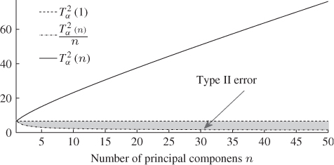
The definition of the χ2 PDF, however, describes the sum of statistically independent Gaussian distributed variables of zero mean and unity variance. In this regard, each element of this sum has the same contribution to the overall statistic. Consequently, the critical contribution of a particular element is the ratio of the control limit over the number of sum elements. On the other hand, testing the alternative hypothesis that a single t-score variable, which follows a Gaussian distribution of zero mean and unity variance and its squared values asymptotically follows a χ2 distribution with 1 degree of freedom, against the control limit of just this one variable can yield a significant Type II error, which Figure 3.2 shows.
Figure 3.2 Type II error for incorrectly applying hypothesis test in Equation (3.37).
The answer to the second question lies in revisiting the term in (3.40)
3.41 
From the above equation, it follows that the contribution of the jth process variable upon the Hotelling's T2 statistic detecting an abnormal condition is equal to
3.42 ![]()
Now, including terms in the above sum that have a different sign to ![]() reduces the overall value of
reduces the overall value of ![]() . Consequently, to identify the main contributors to the absolute value of
. Consequently, to identify the main contributors to the absolute value of ![]() requires the removal of negative sum elements
requires the removal of negative sum elements ![]() .
.
3.2.1.2 Variable contribution to the Q statistic
Given that the Q statistic relies on the sum of the residuals for each variable, the variable contribution of the jth variable is simply (Yoon and MacGregor 2001):
Alternative forms are discussed in Kourti (2005), ![]() , or Chiang et al. (2001),
, or Chiang et al. (2001), ![]() . Since the variance for these residuals may vary, it is difficult to compare them without scaling. Furthermore, using squared values does not offer the possibility of evaluating whether whether a temperature reading is larger or smaller then expected, for example. This suggests that (3.43) should be
. Since the variance for these residuals may vary, it is difficult to compare them without scaling. Furthermore, using squared values does not offer the possibility of evaluating whether whether a temperature reading is larger or smaller then expected, for example. This suggests that (3.43) should be
3.44 
3.2.1.3 Degree of reliability of contribution charts
Although successful diagnoses using contribution charts have been reported (Martin et al. 2002; Pranatyasto and Qin 2001; Vedam and Venkatasubramanien 1999; Yoon and MacGregor 2001), subsection 3.3.1 shows that the PCA residuals of the process variables are linearly dependent. The same analysis can also be applied to show that the recorded process variables have a linearly dependent contribution to the Hotelling's T2 statistic. Moreover, Yoon and MacGregor (2001) discussed that contribution charts generally stem from an underlying correlation model of the recorded process variables which may not possess a causal relationship.
However, contribution charts can identify which group(s) of variables are mostly affected by a fault condition. Lieftucht et al. (2006a) highlighted that the number of degrees of freedom in the residual subspace is an important factor for assessing the reliability of Q contribution charts. The ratio ![]() is therefore an important index to determine the reliability of these charts. The smaller this ratio the larger is the dimension of the residual subspace and the less the degree of linear dependency among the variable contribution to the Q statistic.
is therefore an important index to determine the reliability of these charts. The smaller this ratio the larger is the dimension of the residual subspace and the less the degree of linear dependency among the variable contribution to the Q statistic.
Chapters 4 and 5 demonstrate how contribution charts can assist the diagnosis of fault conditions ranging from simple sensor or actuator faults to more complex process faults. It is important to note, however, that the magnitude of the fault condition can generally not be estimated through the use of contribution charts. Subsection 3.2.3 introduces the projection- and regression-based variable reconstruction that allows determining the kind and size of complex fault scenarios. The next subsection describes residual-based tests to diagnose abnormal process conditions.
3.2.2 Residual-based tests
Wise et al. (1989a) and Wise and Gallagher (1996) introduced residual-based tests that relate to the residuals of a PCA model. Residual-based tests for PLS models can be developed as a project in the tutorial session at the end of the chapter. Preliminaries for calculating the error variance are followed here by outlining the hypothesis tests for identifying which variable is affected by an abnormal operating condition.
3.2.2.1 Preliminaries
The residual variance for recovering the jth process variable, ![]() , is
, is

where ![]() is the jth row vector stored in
is the jth row vector stored in ![]() . Equation (3.45) follows from the fact that
. Equation (3.45) follows from the fact that ![]() , that the t-score variables are statistically independent and that each error variable has the variance
, that the t-score variables are statistically independent and that each error variable has the variance ![]() . If
. If ![]() is unknown, it can be estimated from
is unknown, it can be estimated from ![]() ,
,
3.46 
That ![]() follows from
follows from ![]() and the fact that the p-loading vectors are mutually orthonormal. Equation (2.122) points out that
and the fact that the p-loading vectors are mutually orthonormal. Equation (2.122) points out that ![]() is equal to the sum of the diagonal elements of
is equal to the sum of the diagonal elements of ![]() , which yields
, which yields
Equation (3.47) only requires the first n eigenvalues and eigenvectors of ![]() .
.
Assuming that the availability of a data set of Kf samples describing an abnormal operating condition and a second data set of normal process behavior containing K samples, it is possible to calculate the following ratio which follows an F-distribution
3.48 
where both variances can be computed from their respective data sets. This allows testing the null hypothesis that the jth variable is not affected by a fault condition
or the alternative hypothesis that this variable is affected
3.50 
Testing the null hypothesis can only be performed if the last nz − n eigenvalues are identical, that is, the variance of the error variables are identical. If this is not the case, however, the simplification leading to (3.47) cannot be applied and the variance of each residual must be estimated using computed residuals. A procedure for determining which variable is affected by a fault condition is given next.
3.2.2.2 Variable contribution to detected fault condition
The mean for each of the residuals is zero
3.51 ![]()
which can be taken advantage of in testing whether a statistically significant departure in mean occurred. This is a standard test that is based on the following statistic
3.52 
where ![]() is the mean estimated from the Kf samples describing a fault condition. This statistic follows a t-distribution with the following upper and lower control limit
is the mean estimated from the Kf samples describing a fault condition. This statistic follows a t-distribution with the following upper and lower control limit
3.53 ![]()
for a significance α. The null hypothesis, H0, is therefore
3.54 
The alternative hypothesis, H1 is accepted if
By inspecting the above hypothesis tests in (3.49) and (3.55) for changes in the error variance and the mean of the error variables for recovering the recorded process variables, it is apparent that they require a set of recorded data that describes the fault condition. This, however, hampers the practical usefulness of these residual-based tests given that a root cause analysis should be conducted upon detection of a fault condition. Such immediate analysis can be offered by contribution charts and variable reconstruction charts that are discussed next.
3.2.3 Variable reconstruction
Variable reconstruction exploits the correlation among the recorded process variables and hence, variable interrelationships. This approach is closely related to the handling of missing data in multivariate data analysis (Arteaga and Ferrer 2002; Nelson et al. 1996; Nelson et al. 2006) and relies on recovering the variable set z0 and x0 based on the n source variables of the PCA and PLS data structures, respectively
According to 2.2 and 2.24, ![]() and
and ![]() mainly describe the impact of the common-cause variation, Ξs and
mainly describe the impact of the common-cause variation, Ξs and ![]() , upon z0 and x0, respectively.
, upon z0 and x0, respectively.
3.2.3.1 Principle of variable reconstruction
For PCA, the derivation below shows how to reconstruct a subset of variables in z0. A self-study project in the tutorial section aims to develop a reconstruction scheme for PLS. Under the assumption that n < nz, it follows from (3.56) that
3.57 
which can be rewritten to become
3.58 ![]()
where ![]() ,
, ![]() ,
, ![]() and
and ![]() . The linear dependency between the elements of
. The linear dependency between the elements of ![]() follow from
follow from
3.59 ![]()
The above partition of the loading matrix into the first n rows and the remaining nz − n rows is arbitrary. By rearranging the row vectors of P along with the elements of ![]() any nz − n elements in
any nz − n elements in ![]() are linearly dependent on the remaining n elements. Subsection 3.3.1 discusses this in more detail.
are linearly dependent on the remaining n elements. Subsection 3.3.1 discusses this in more detail.
Nelson et al. (1996) described three different techniques to handle missing data. The analysis in Arteaga and Ferrer (2002) showed that two of them are projection-based while the third one uses regression. Variable reconstruction originates from the projection-based approach for missing data, which is outlined next. The regression-based reconstruction is then presented, which isolates deterministic fault signatures from the t-score variables and removes such signatures from the recorded data.
3.2.3.2 Projection-based variable reconstruction
The principle of projection-based variable reconstruction is best explained here by a simple example. This involves two highly correlated process variables, z1 and z2. For a high degree of correlation, Figure 2.1 outlines that a single component can recover the value of both variables without a significant loss of accuracy. The presentation of the simple introductory example is followed by a regression-based formulation of projecting samples optimally along predefined directions. This is then developed further to directly describe the effect of the sample projection upon the Q statistic. Next, the concept of reconstructing single variables is extended to include general directions that describe a fault subspace. Finally, the impact of reconstructing a particular variable upon the Hotelling's T2 and Q statistics is analyzed and a regression-based reconstruction approach is introduced for isolating deterministic fault conditions.
An introductory example
Assuming that the sensor measuring variable z1 produces a bias that takes the form of a step (sensor bias), the projection of the data vector ![]() onto the semimajor of the control ellipse yields
onto the semimajor of the control ellipse yields
with Δz1 being the magnitude of the sensor bias. Using the score variable tf to recover the sensor readings gives rise to
The recovered values are therefore
3.62 
This shows that the recovery of the value of both variables is affected by the sensor bias of z1. The residuals of both variables are also affected by this fault
since
3.64 ![]()
Subsection 3.3.1 examines dependencies in variable contributions to fault conditions, a general problem for constructing contribution charts (Lieftucht et al. 2006a; Lieftucht et al. 2006b).
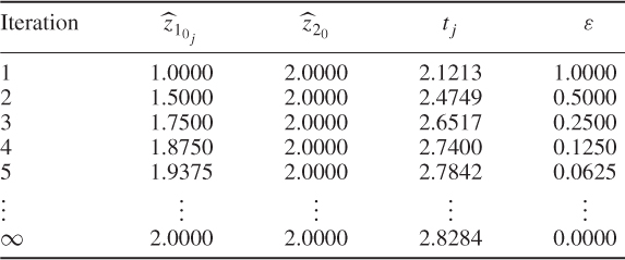
The application of projection-based variable reconstruction, however, can overcome this problem if the fault direction is known a priori (Dunia et al. 1996; Dunia and Qin 1998) or can be estimated (Yue and Qin 2001) using a singular value decomposition. The principle is to remove the faulty sensor reading for z1 by an estimate, producing the following iterative algorithm
The iteration converges for j → ∞ and yields the following estimate for ![]()
On the other hand, if a sensor bias is affecting z2 the estimate ![]() is then
is then
3.67 ![]()
Figure 3.3 presents an example where the model subspace is spanned by ![]() and a data vector
and a data vector ![]() describes a sensor bias to the first variables,
describes a sensor bias to the first variables, ![]() . The series of arrows show the convergence of this iterative algorithm. Applying this scheme for
. The series of arrows show the convergence of this iterative algorithm. Applying this scheme for ![]() , Table 3.1 shows how
, Table 3.1 shows how ![]() ,
, ![]() ,
, ![]() and the convergence criterion
and the convergence criterion ![]() changes for the first few iteration steps. According to Figure 3.3 and Table 3.1, the ‘corrected’ or reconstructed data vector is
changes for the first few iteration steps. According to Figure 3.3 and Table 3.1, the ‘corrected’ or reconstructed data vector is ![]() .
.
Figure 3.3 Illustrative example of projection-based variable reconstruction.

Table 3.1 Results of reconstructing z10 using the iterative projection-based method
Regression-based formulation of projection-based variable reconstruction
In a similar fashion to the residual-based tests in Subsection 3.2.2, it is possible to formulate the projection-based variable reconstruction scheme as a least squares problem under the assumptions that:
- the fault condition affects at most n sensors;
- the fault signature manifest itself as a step-type fault for the affected variables; and
- a recorded data set contains a sufficiently large set of samples representing the fault condition.
A sensor bias that affects the mth variable can be modeled as follows
where ![]() is an Euclidian vector for which the mth element is 1 and the remaining ones are 0, and Δzm is the magnitude of the sensor bias. The difference between the measured data vector
is an Euclidian vector for which the mth element is 1 and the remaining ones are 0, and Δzm is the magnitude of the sensor bias. The difference between the measured data vector ![]() and
and ![]() is the Gaussian distributed vector
is the Gaussian distributed vector ![]() , whilst the
, whilst the ![]() is Gaussian distributed with the same covariance matrix, that is,
is Gaussian distributed with the same covariance matrix, that is, ![]() , which follows from the data model in 2.2 and Table 2.1. This implies that the fault magnitude, Δzm, can be estimated if the fault direction
, which follows from the data model in 2.2 and Table 2.1. This implies that the fault magnitude, Δzm, can be estimated if the fault direction ![]() is known by the following least squares formulation
is known by the following least squares formulation
The solution of (3.69) is the estimate of the mean value for ![]()

which converges to the true fault magnitude as ![]() .
.
Impact of fault condition upon Q statistic
Dunia and Qin (1998) showed that projecting samples along ![]() has the following impact on the Q statistic
has the following impact on the Q statistic
Knowing that ![]() , (3.71) becomes
, (3.71) becomes
where ![]() . It follows from (3.72) that if
. It follows from (3.72) that if
3.73 ![]()
Δzm asymptotically converges to the true fault magnitude allowing a complete isolation between the step-type fault and normal stochastic process variation, hence
3.74 
The optimal solution of the objective function in (3.71) is given by

The estimates for Δzm in (3.70) and (3.75) are identical. To see this, the sensor bias upon has the following impact on the residuals
3.76 ![]()
which we can substitute into the expectation of (3.75)
3.77 
Geometrically, the fault condition moves the samples along the direction ![]() and this shift can be identified and removed from the recorded data.
and this shift can be identified and removed from the recorded data.
Extension to multivariate fault directions
A straightforward extension is the assumption that ![]() sensor faults arise at the same time. The limitation
sensor faults arise at the same time. The limitation ![]() follows from the fact that the rank of P is n and is further elaborated in Subsection 3.3.2. The extension of reconstructing up to n variables would enable the description of more complex fault scenarios. This extension, however, is still restricted by the fact that the fault subspace, denoted here by
follows from the fact that the rank of P is n and is further elaborated in Subsection 3.3.2. The extension of reconstructing up to n variables would enable the description of more complex fault scenarios. This extension, however, is still restricted by the fact that the fault subspace, denoted here by ![]() , is spanned by Euclidian vectors
, is spanned by Euclidian vectors
3.78 ![]()
where ![]() is an index set storing the variables to be reconstructed, for example
is an index set storing the variables to be reconstructed, for example ![]() ,
, ![]() , ··· ,
, ··· , ![]() . The case of
. The case of ![]() storing non-Euclidian vectors is elaborated below. Using the fault subspace
storing non-Euclidian vectors is elaborated below. Using the fault subspace ![]() projection-based variable reconstruction identifies the fault magnitude for each Euclidian base vector from the Q statistic
projection-based variable reconstruction identifies the fault magnitude for each Euclidian base vector from the Q statistic

Here, ![]() . The solution for the least squares objective function is
. The solution for the least squares objective function is
3.80 
with ![]() being the generalized inverse of
being the generalized inverse of ![]() . If
. If ![]() is the correct fault subspace, the above sum estimates the fault magnitude
is the correct fault subspace, the above sum estimates the fault magnitude ![]() consistently
consistently
3.81 
since
3.82 
This, in turn, implies that the correct fault subspace allows identifying the correct fault magnitude and removing the fault information from the Q statistic
3.83 ![]()
So far, we assumed that the fault subspace is spanned by Euclidian vectors that represent individual variables. This restriction can be removed by defining a set of up to ![]() linearly independent vectors
linearly independent vectors ![]() ,
, ![]() , … ,
, … , ![]() of unit length, which yields the following model for describing fault conditions
of unit length, which yields the following model for describing fault conditions
3.84 ![]()
The fault magnitude in the direction of vector ![]() is
is ![]() . The
. The ![]() vectors can be obtained by applying a singular value decomposition on the data set containing
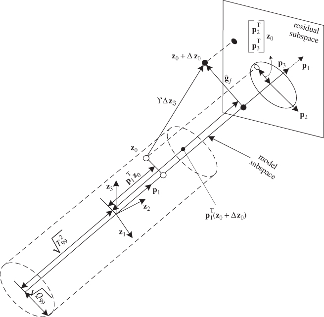
vectors can be obtained by applying a singular value decomposition on the data set containing ![]() samples describing the fault condition (Yue and Qin 2001). Figure 3.4 gives a graphical interpretation of this regression problem. Equation (3.79) presents the associated objective function for estimating
samples describing the fault condition (Yue and Qin 2001). Figure 3.4 gives a graphical interpretation of this regression problem. Equation (3.79) presents the associated objective function for estimating ![]() . Different from the projection along Euclidian directions, if the fault subspace is constructed from non-Euclidian vectors, the projection-based variable reconstruction constitutes an oblique projection.
. Different from the projection along Euclidian directions, if the fault subspace is constructed from non-Euclidian vectors, the projection-based variable reconstruction constitutes an oblique projection.
Figure 3.4 Graphical illustration of multivariate projection-based variable reconstruction along a predefined fault axis.
Projection-based variable reconstruction for a single sample
As for residual-based tests, the above projection-based approach requires a sufficient number of samples describing the fault condition, which hampers its practical usefulness. If an abnormal event is detected, the identification of potential root causes is vital in order to support process operators in carrying out appropriate responses. Despite the limitations of contribution charts, discussed in (Lieftucht et al. 2006a; Yoon and MacGregor 2001) and Subsection 3.3.1, they should be used as a first instrument.
Equations (3.60) to (3.66) show that a sensor bias can be removed if it is known which one is faulty. Dunia and Qin (1998), and Lieftucht et al. (2006b) pointed out that projection-based reconstruction and contribution charts can be applied together to estimate the impact of a fault condition upon individual process variables. A measure for assessing this impact is how much the reconstructed variable reduces the value of both non-negative quadratic statistics. For the Q statistic, this follows from (3.72) for ![]() and
and ![]() , and (3.79) for
, and (3.79) for ![]() .
.
As highlighted in Lieftucht et al. (2006a), however, the projection-based reconstruction impacts the geometry of the PCA model and therefore the non-negative quadratic statistics. Subsection 3.3.2 describes the effect of reconstructing a variable set upon the geometry of the PCA model. In summary, the procedure to incorporate the effect of projecting a set of ![]() process variables is as follows.
process variables is as follows.
3.85 
 ;
; ;
; is a data vector that stores the variables to be reconstructed as the first
  elements,
  , and the variables that are not reconstructed as the remaining
  elements,
  ;
;- the matrices denoted by the superscript * refer to the variables stored in the rearranged vector
 ;
; - the symbol
 refers to the reconstructed portions of the data covariance matrix describing the impact of reconstructing the set of
  process variables;
  is the partition of the data covariance matrix
  that relates to the variable set that is not reconstructed; and
- the indices 1, 2 and 3 are associated with the covariance matrix of the reconstructed variables, the cross covariance matrix that includes the reconstructed and the remaining variables and the covariance matrix of the unreconstructed variables, respectively.
Ignoring the effect the reconstruction process imposes upon the underlying PCA model is demonstrated in Chapter 4.
Limitations of projection-based variable reconstruction
Despite the simplicity and robustness of the projection-based variable reconstruction approach, it is prone to the following problems (Lieftucht et al. 2009).
These problems are demonstrated in Lieftucht et al. (2009) through the analysis of experimental data from a reactive distillation column. A regression-based variable reconstruction is introduced next to address these problems.
3.2.3.3 Regression-based variable reconstruction
This approach estimates and separates the fault signature from the recorded variables (Lieftucht et al. 2006a; Lieftucht et al. 2009). Different from projection-based reconstruction, the regression-based approach relies on the following assumptions:
- The fault signature in the score space,
 , is deterministic, that is, the signature for a particular process variable is a function of the sample index k; and
 - The fault is superimposed onto the process variables, that is, it is added to the complete set of score variables
3.86 ![]()
 ; and
; and .
.
In contrast to the regression-based technique for missing data, different assumptions are applied to the score variables leading to a method for variable reconstruction according to Figure 3.5. Based on the above assumptions, the fault signature can be described by a parametric curve that can be identified using various techniques, such as polynomials, principal curves and artificial neural networks (Walczak and Massart 1996). For simplicity, radial basis function networks (RBFNs) are utilized here.
Figure 3.5 Structure of the regression based variable reconstruction technique.
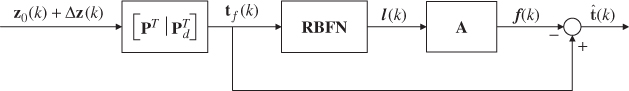
According to Figure 3.5, ![]() is subtracted from
is subtracted from ![]() . The benefit of using the score variables follows from Theorem 9.3.2. The score variables are statistically independent but the original process variables are highly correlated. Equations (3.61) and (3.63) describe the negative impact of variable correlation upon the PCA model, which not only identify a faulty sensor but may also suggest that other variables are affected by a sensor bias. Separating the fault signature from the corrupted samples on the basis of the score variables, however, circumvents the correlation issue.
. The benefit of using the score variables follows from Theorem 9.3.2. The score variables are statistically independent but the original process variables are highly correlated. Equations (3.61) and (3.63) describe the negative impact of variable correlation upon the PCA model, which not only identify a faulty sensor but may also suggest that other variables are affected by a sensor bias. Separating the fault signature from the corrupted samples on the basis of the score variables, however, circumvents the correlation issue.
The first block in Figure 3.5 produces the complete set of nz score variables f(k) from the corrupted samples of the process variables ![]() . The score variable set is then used to estimate the fault signature
. The score variable set is then used to estimate the fault signature ![]() as above which is subtracted from the score variables to estimate
as above which is subtracted from the score variables to estimate ![]() . Since a fault signature may affect each of the score variables, all score variables need to be included to estimate the fault signature.
. Since a fault signature may affect each of the score variables, all score variables need to be included to estimate the fault signature.
The output from a radial basis function network is defined by
Here, R is the number of network nodes, ![]() , 1 ≤ j ≤ nz, 1 ≤ i ≤ R is a Gaussian basis function for which ci and
, 1 ≤ j ≤ nz, 1 ≤ i ≤ R is a Gaussian basis function for which ci and ![]() are the center and the width, respectively, and
are the center and the width, respectively, and ![]() are the network weights. By applying (3.87), the separation of the fault signature becomes
are the network weights. By applying (3.87), the separation of the fault signature becomes
3.88 ![]()
where, ![]() is a vector storing the values for each network node for the kth sample, A is a parameter matrix storing the network weights and
is a vector storing the values for each network node for the kth sample, A is a parameter matrix storing the network weights and ![]() is the isolated stochastic part of the computed score variables tf(k). For simplicity, the center of Gaussian basis functions is defined by a grid, that is, the distance between two neighboring basis functions is equivalent for each pair and their widths are assumed to be predefined. The training of the network therefore reduces to a least squares problem.
is the isolated stochastic part of the computed score variables tf(k). For simplicity, the center of Gaussian basis functions is defined by a grid, that is, the distance between two neighboring basis functions is equivalent for each pair and their widths are assumed to be predefined. The training of the network therefore reduces to a least squares problem.
Chapter 4 shows that the regression-based reconstruction has the potential to provide a clear picture of the impact of a fault condition. Lieftucht et al. (2009) present another example that involves recorded data from an experimental reactive distillation unit at the University of Dortmund, Germany, where this technique could offer a good isolation of the fault signatures for a failure in the reflux preheater and multiple faults in cooling water and acid feed supplies.
3.3 Geometry of variable projections
For the projection-based reconstruction of a single sample, this section analyzes the geometry of variable projections, which involves orthogonal projections from the original variable space onto smaller dimensional reconstruction subspaces that capture significant variation in the original variable set. Subsection 3.3.1 examines the impact of such projections upon the contribution charts of the Q statistic for PCA and PLS and shows that the variable contributions are linearly dependent. This is particularly true if the number of retained components is close to the size of the original variable set. Subsection 3.3.2 then studies the impact of variable reconstruction upon the geometry of the PCA model.
3.3.1 Linear dependency of projection residuals
Given the PCA residual vector ![]() and the centered data vector
and the centered data vector ![]() , it is straightforward to show that the residual vector is orthogonal to the model subspace
, it is straightforward to show that the residual vector is orthogonal to the model subspace
Here, ![]() , is the loading matrix, storing the eigenvectors of the data covariance matrix as column vectors, which span the model plane. The above relationship holds true, since the eigenvectors of a symmetric matrix are mutually orthonormal. Equation (3.89), however, can be further elaborated
, is the loading matrix, storing the eigenvectors of the data covariance matrix as column vectors, which span the model plane. The above relationship holds true, since the eigenvectors of a symmetric matrix are mutually orthonormal. Equation (3.89), however, can be further elaborated
3.90 
and partitioning it as follows
3.91 
which gives rise to
3.92 ![]()
Ψ1 is a square matrix and can be inverted, which yields
3.93 ![]()
The above relationship is not dependent upon the number of source signals n. In any case there will be a linear combination of the variable contribution of the Q statistic.
3.3.2 Geometric analysis of variable reconstruction
The geometrical properties of the multidimensional reconstruction technique for a single sample are now analyzed. Some preliminary results for one-dimensional sensor faults were given in Lieftucht et al. (2004) and a more detailed analysis is given in Lieftucht et al. (2006a). For simplicity, the data vector z0 is rearranged such that the reconstructed variables are stored as the first ![]() elements. The rearranged vector and the corresponding covariance and loading matrix are denoted by
elements. The rearranged vector and the corresponding covariance and loading matrix are denoted by ![]() ,
, ![]() and P*, respectively. Furthermore, the reconstructed vector and the reconstructed data covariance and loading matrices are referred to as
and P*, respectively. Furthermore, the reconstructed vector and the reconstructed data covariance and loading matrices are referred to as ![]() ,
, ![]() and
and ![]() , respectively.
, respectively.
3.3.2.1 Optimality of projection-based variable reconstruction
The following holds true for the reconstructed data vector and the model subspace.
3.94 ![]()
3.96 
3.97 ![]()
3.98 
3.99 ![]()
3.100 ![]()
3.3.2.2 Reconstruction subspace
The data vector ![]() but the reconstruction of
but the reconstruction of ![]() to form
to form ![]() results in a projection of
results in a projection of ![]() onto a
onto a ![]() -dimensional subspace, which Theorem 3.3.2 formulates. Any sample
-dimensional subspace, which Theorem 3.3.2 formulates. Any sample ![]() is projected onto this reconstruction subspace along the
is projected onto this reconstruction subspace along the ![]() directions defined in ϒ. As Theorem 3.3.1 points out, the distance of the reconstructed sample and the model subspace is minimal.
directions defined in ϒ. As Theorem 3.3.1 points out, the distance of the reconstructed sample and the model subspace is minimal.
3.102 ![]()
3.103 
3.3.2.3 Maximum dimension of fault subspace
Theorem 3.3.3 discusses the maximum dimension of the fault subspace.
3.105 ![]()
3.106 ![]()
3.108 
3.109 
3.110 ![]()
3.111 
3.112 
3.3.2.4 Influence on the data covariance matrix
For simplicity, the analysis in the remaining part of this subsection assumes that ϒ stores Euclidian column vectors. It is, however, straightforward to describe the impact of the projection-based reconstruction upon the data covariance matrix if ϒ includes non-Euclidian column vectors, which is a project in the tutorial session. Variable reconstruction leads to changes of the data covariance matrix which therefore must be reconstructed. Partitioning the rearranged data covariance matrix ![]()
3.113 
where ![]() and
and ![]() and
and ![]() , the reconstruction of
, the reconstruction of ![]() affects the first two matrices,
affects the first two matrices, ![]() and
and ![]()
and
3.115 ![]()
where ![]() , and
, and ![]() and
and ![]() are the covariance and cross-covariance matrices involving
are the covariance and cross-covariance matrices involving ![]() . Replacing
. Replacing ![]() by
by ![]() and
and ![]() by
by ![]()
yields the following corollary.
The effect of variable reconstruction upon the model and residual subspaces, which are spanned by eigenvectors of ![]() , is analyzed in the following subsections.
, is analyzed in the following subsections.
3.3.2.5 Influence on the model plane
Pearson (1901) showed that the squared length of the residual vector between K mean-centered and scaled data points of dimension nz and a given model subspace of dimension n is minimized if the model subspace is spanned by the first-n dominant eigenvectors of the data covariance matrix. Theorems 3.3.1 and 3.3.2 highlight that projecting samples onto the subspace Π leads to a minimum distance between the projected points and the model subspace. This gives rise to the following theorem.
The above theorem follows from the work of Pearson (1901), given that the reconstructed samples have a minimum distance from the original model subspace.
The above corollary is a result of the changes that the reconstruction procedure imposes on ![]() , which may affect the eigenvectors and the eigenvalues.
, which may affect the eigenvectors and the eigenvalues.
The influence of the projection onto the residual subspace is discussed next.
3.3.2.6 Influence on the residual subspace
Following from the preceding discussion, the reconstruction results in a shift of a sample in the direction of the fault subspace, such that the squared length of the residual vector is minimal (Theorem 3.3.1). Since the reconstruction procedure is, in fact, a projection of z0 onto Π, which is of dimension ![]() (Theorem 3.3.2), it follows that the dimension of the residual subspace is
(Theorem 3.3.2), it follows that the dimension of the residual subspace is ![]() , because the dimension of the model subspace remains unchanged.
, because the dimension of the model subspace remains unchanged.
Since the model subspace is assumed to describe the linear relationships between the recorded and source variables, which follows from Equation (2.2), the ![]() discarded eigenvalues represent the cumulative variance of the residual vector. Moreover, given that
discarded eigenvalues represent the cumulative variance of the residual vector. Moreover, given that ![]() has a rank of
has a rank of ![]() ,
, ![]() eigenvalues are equal to zero.
eigenvalues are equal to zero.
An example to illustrate the effect of the above corollaries is given in Chapter 4. It is important to note that even if the projection-based variable reconstruction has only minor effect on the data covariance matrix, this influence will lead to changes of the monitoring statistics and their confidence limits, which is examined next.
3.3.2.7 Influence on the monitoring statistics
The impact of variable reconstruction manifests itself in the construction of ![]() , which yields a different eigendecomposition. Since the Hotelling's T2 and the Q statistic are based on this eigendecomposition, it is necessary to account for such changes when applying projection-based variable reconstruction. For reconstructing a total of
, which yields a different eigendecomposition. Since the Hotelling's T2 and the Q statistic are based on this eigendecomposition, it is necessary to account for such changes when applying projection-based variable reconstruction. For reconstructing a total of ![]() variables, this requires the following steps to be carried out:
variables, this requires the following steps to be carried out:
This procedure allows establishing reliable monitoring statistics for using projection-based variable reconstruction. If the above procedure is not followed, the variance of the score variables, the loading vectors and the variance of the residuals are incorrect, which yields erroneous results (Lieftucht et al. 2006a).
3.4 Tutorial session
Question 1:
What is the advantage of assuming a Gaussian distribution of the process variables for constructing monitoring charts?
Question 2:
With respect to the data structure in 2.2, develop fault conditions that do not affect (i) the Hotelling's T2 statistic and (ii) the residual Q statistic. Provide general fault conditions which neither statistic is sensitive to.
Question 3:
Considering that the Hotelling's T2 and Q statistics are established on the basis of the eigendecomposition of the data covariance matrix, is it possible to construct a fault condition that neither affects the Hotelling's T2 nor the Q statistic?
Question 4:
Provide a proof of (3.27).
Question 5:
Provide proofs for (3.72) and (3.75).
Question 6:
For projections along predefined Euclidean axes for single samples, why does variable reconstruction affect the underlying geometry of the model and residual subspaces?
Question 7:
Following from Question 6, why is the projection-based approach for multiple samples not affected by variable reconstruction to the same extent as the single-sample approach? Analyze the asymptotic properties of variable reconstruction.
Question 8:
Excluding the single-sample projection-based approach, what is the disadvantage of projection- and regression-based variable reconstruction over contribution charts?
Project 1:
With respect to Subsection 3.2.2, develop a set of residual-based tests for PLS.
Project 2:
For PCA, knowing that ![]() ,
, ![]() and
and ![]() , design an example that describes a sensor fault for the first variable but for which the contribution chart for the Q statistic identifies the second variable as the dominant contributor to this fault. Can the same problem also arise with the use of the residual-based tests in Subsection 3.2.2? Check your design by a simulation example.
, design an example that describes a sensor fault for the first variable but for which the contribution chart for the Q statistic identifies the second variable as the dominant contributor to this fault. Can the same problem also arise with the use of the residual-based tests in Subsection 3.2.2? Check your design by a simulation example.
Project 3:
With respect to Subsection 3.2.3, develop a variable reconstruction scheme for the input variable set of a PLS model. How can a fault condition for the output variable set be diagnosed?
Project 4:
Simulate an example involving 3 process variables that is superimposed by a fault condition described by ![]() ,
, ![]() ,
, ![]() ,
, ![]() and develop a reconstruction scheme to estimate the fault direction
and develop a reconstruction scheme to estimate the fault direction ![]() and the fault magnitude Δzυ.
and the fault magnitude Δzυ.
Project 5:
Using a simulation example that involves 3 process variables, analyze why projection-based variable reconstruction is not capable of estimating the fault signature is not of the form ![]() , i.e.
, i.e. ![]() , with Δz(k) being a deterministic sequence. Contrast the performance of the regression-based variable reconstruction scheme with that of the projection-based scheme? How can a fault condition be diagnosed if it is of the form Δz(k) but stochastic in nature?
, with Δz(k) being a deterministic sequence. Contrast the performance of the regression-based variable reconstruction scheme with that of the projection-based scheme? How can a fault condition be diagnosed if it is of the form Δz(k) but stochastic in nature?
Notes
1 For a central χ2 distribution, the mean of each contributing element is assumed to be zero unlike a noncentral where this assumption is relaxed.
2 The mean and variance of χ2(h), E{χ2(h)} and E{(χ2(h) − h)2}, are h and 2h, respectively.