 CHAPTER 6
Motion Planning for Three-Dimensional Arm Manipulators
The robot is going to lose. Not by much. But when the final score is tallied, flesh and blood is going to beat the damn monster.
—Adam Smith, philosopher and economist, 1723–1790
6.1 INTRODUCTION
We are continuing developing SIM (Sensing–Intelligence–Motion) algorithms for robot arm manipulators. The cases considered in Chapter 5 all deal with arm manipulators whose end effectors (hands) move along a two-dimensional (2D) surface. Although applications do exist that can make use of those algorithms—for example, assembly of microelectronics on a printed circuit board is largely limited to a 2D operation—most robot arm manipulators live and work in three-dimensional (3D) space. From this standpoint, our primary objective in Chapter 5 should be seen as preparing the necessary theoretical background and elucidating the relevant issues, before proceeding to the 3D case. Sensor-based motion planning algorithms should be able to handle 3D space and 3D arm manipulators. Developing such strategies is the objective of this chapter. As before, the arm manipulators that we consider are simple open kinematic chains.
Is there a fundamental difference between motion planning for two-dimensional (2D) and 3D arm manipulators? The short answer is yes, but the question is not that simple. Recall a similar discussion about mobile robots in Chapter 3. From the standpoint of motion planning, mobile robots differ from arm manipulators: They have more or less compact bodies, kinematics plays no decisive role in their motion planning, and their workspace is much larger compared to their dimensions. For mobile robots the difference between the 2D and 3D cases is absolute and dramatic: Unequivocally, if the 2D case has a definite and finite solution to the planning problem, the 3D case has no finite solution in general.
The argument goes as follows. Imagine a bug moving in the two-dimensional plane, and imagine that on its way the bug encounters an object (an obstacle). Assume the bug's target location is somewhere on the other side of the obstacle. One way for it to continue its motion is to first pass around the obstacle. The bug has only two options: It can pass the obstacle from the left or it can pass it from the right, clockwise or counterclockwise. If neither option leads to success—let us assume it is a smart bug, with a reasonably good motion planning skills—the goal is not achievable. In this case, by slightly exaggerating the bug's stubbornness, we will note that eventually the bug will come back to the point on the obstacle where it started. It took only one simple going around, all in one direction, to explore the whole obstacle. That is the essence of the 2D case.
Imagine now a fly that is flying around a room—that is, in 3D space. Imagine that on its way the fly encounters a (3D) obstacle—say, a child's balloon hanging on a string. Now there is an infinite number of routes the fly can take to pass around the obstacle. The fly would need to make a great many loops around the obstacle in order to explore it completely. That's the fundamental difficulty of the 3D case; in theory it takes an infinitely long path to explore the whole obstacle, even if its dimensions and volume are finite and modest.1 The point is that while in the 2D case a mobile robot has a theoretically guaranteed finite solution, no such solution can be guaranteed for a 3D mobile robot. The 3D sensor-based motion planning problem is in general intractable.
The situation is more complex, but also not as hopeless, for 3D arm manipulators. Try this little experiment. Fix your shoulder and try to move your hand around a long vertical pole. Unlike a fly that can make as many circles around the pole as it wishes, your hand will make about one circle around the pole and stop. What holds it from continuing moving in the same direction is the arm's kinematics and also the fact that the arm's base is “nailed down.” The length of your arm links is finite, the links themselves are rigid, and the joints that connect the links allow only so much motion. These are natural constraints on your arm movement. The same is so for robot arm manipulators. In other words, the kinematic constraints of an arm manipulator impose strong limitations on its motion.
This fact makes the problem of sensor-based motion planning for 3D arm manipulators manageable. The hope is that the arm kinematics can be effectively exploited to make the problem tractable. Furthermore, those same constraints promise a constructive test of target reachability, similar to those we designed above for mobile robots and 2D arm manipulators.
As noted by Brooks [102], the motion planning problem for a manipulator with revolute joints is inherently difficult because (a) the problem is nondecomposable, (b) there may be difficulties associated with rotations, (c) the space representation and hence the time execution of the algorithm are exponential in the number of robot's degrees of freedom of the objects involved, and (d) humans are especially poor at the task when much reorientation is needed, which makes it difficult to develop efficient heuristics. This is all true, and indeed more true for arms with revolute joints—but these difficulties have been formulated for the motion planning problem with complete in formation. Notice that these difficulties above did not prevent us from designing rather elegant sensor-based planning algorithms for 2D arms with revolute joints, even in the workspace with arbitrarily complex obstacles. The question now is how far we can go with the 3D case.
It was said before that this is a difficult area of motion control and algorithm design. As we will see in Chapter 7, human intuition is of little help in designing reasonable heuristics and even in assessing proposed algorithms. Doing research requires expertise from different areas, from topology to sensing technology. There are still many unclear issues. Much of the exciting research is still waiting to be done. Jumping to the end of this chapter, today there are still no provable algorithms for the 3D kinematics with solely revolute joints. While this type of kinematics is just one mechanism among others in today's robotics, it certainly rules the nature.
As outlined in Section 5.1.1, we use the notion of a separable arm [103], which is an arm naturally divided into the major linkage responsible for the arm's position planning (or gross motion), and the minor linkage (the hand) responsible for the orientation planning of the arm's end effector. As a rule, existing arm manipulators are separable. Owing to the fact that three degrees of freedom (DOF) is the minimum necessary for reaching an arbitrary point in 3D space, and another three DOF are needed to provide an arbitrary orientation for the tool—six DOF in total as a minimum—many 3D arm manipulators' major linkages include three links and three joints, and so do typical robot hands. Our motion planning algorithms operate on the major linkage—that is, on handling gross motion and making sure that the hand is brought into the vicinity of the target position. The remaining “fine tuning” for orientation is usually a simpler task and is assumed to be done outside of the planning algorithm. For all but very few unusual applications, this is a plausible assumption.
While studying topological characteristics of the robot configuration space for a few 3D kinematics types, we will show that obstacle images in these configuration spaces exhibit a distinct property that we call space monotonicity : For any point on the surface of the obstacle image, there exists a direction along which all the remaining points of the configuration space belong to the obstacle. Furthermore, the sequential connection of the arm links results in the property called space anisotropy of the configuration space, whereby the obstacle monotonicity presents itself differently along different space axes.
The space monotonicity property provides a basis for selecting directions of arm motion that are more promising than others for reaching the target position. By exploiting the properties of space monotonicity and anisotropy, we will produce motion planning algorithms with proven convergence. No explicit or implicit beforehand calculations of the workspace or configuration space will be ever needed. All the necessary calculations will be carried out in real time in the arm workspace, based on its sensing information. No exhaustive search will ever take place.
As before with 2D arms, motion planning algorithms that we will design for 3D arms will depend heavily on the underlying arm kinematics. Each kinematics type will require its own algorithm. The extent of algorithm specialization due to arm kinematics will be even more pronounced in the 3D case than in the 2D case. Let us emphasize again that this is not a problem of depth of algorithmic research but is instead a fundamental constraint in the relationship between kinematics and motion. The same is true, of course, in nature: The way a four-legged cat walks is very different from the way a two-legged human walks. Among four-legged, the gaits of cats and turtles differ markedly. One factor here is the optimization process carried out by the evolution. Even if a “one fits all” motion control procedure is feasible, it will likely be cumbersome and inefficient compared to algorithms that exploit specific kinematic peculiarities. We observed this in the 2D case (Section 5.8.4): While we found a way to use the same sensor-based motion planning algorithm for different kinematics types, we also noted the price in inefficiency that this universality carried. Here we will attempt both approaches.
This is not to say that the general approach to motion planning will be changing from one arm to another; as we have already seen, the overall SIM approach is remarkably the same independent of the robot kinematics, from a sturdy mobile robot to a long-limbed arm manipulator.
As before, let letters P and R refer to prismatic and revolute joints, respectively. We will also use the letter X to represent either a P or a R joint, X = [P, R]. A three-joint robot arm manipulator (or the major linkage of an arm), XXX, can therefore be one of eight basic kinematic linkages: PPP, RPP, PRP, RRP, PPR, RPR, PRR, and RRR. As noted in Ref. 111, each basic linkage can be implemented with different geometries, which produces 36 linkages with joint axes that are either perpendicular or parallel to one another. Among these, nine degenerate into linkages with only one or two DOF; seven are planar. By also eliminating equivalent linkages, the remaining 20 possible spatial linkages are further reduced to 12, some of which are of only theoretical interest.
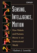
The above sequence XXX is written in such an order that the first four linkages in it are XXP arms; in each of them the outermost joint is a P joint. Those four are among the five major 3D linkages (see Figure 6.1) that are commonly seen in industry [111–113] and that together cover practically all today's commercial and special-purpose robot arm manipulators. It turns out that these four XXP arms are better amenable to sensor-based motion planning than the fifth one (Figure 6.1e) and than the remaining four arms in the XXX sequence. It is XXP arms that will be studied in this chapter.
While formally these four linkages—PPP, RPP, PRP, and RRP—cover a half of the full group XXX, they represent four out of five, or 80%, of the linkages in Figure 6.1. Many, though not all, robot arm applications are based on XXP major linkages. Welding, assembly, and pick-and-place robot arms are especially common in this group, one reason being that a prismatic joint makes it easy to produce a straight-line motion and to expand the operating space. The so-called SCARA arm (Selective Compliance Assembly Robot Arm), whose major linkage is, in our notation, an RRP arm, is especially popular among assembly oriented industrial arm manipulators.
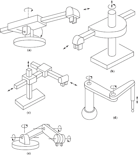
Figure 6.1 Five commonly used 3D robot arm linkages: (a) RRP, “polar coordinates” arm, with a spherical workspace; (b) PRP, “cylindrical coordinates” arm, with a cylindrical workspace; (c) PPP, Cartesian arm, with a “cubicle” workspace; (d) RRP, SCARA-type arm, with a cylindrical workspace; and (e) RRR, “articulate” arm, with a spherical workspace.
Recall our showing in Chapter 5 that RR, the arm with two revolute joints, is the most general among XX arms, X = [P, R]. We will similarly show that the arm RRP is the most general case among XXP arms. The algorithm that works for the RRP arm will work for other XXP arms.
While arm configurations shown in Figure 6.1 have nice straight-line links that are mutually perpendicular or parallel, our SIM approach does not require such properties unless specified explicitly.
We will first analyze the PPP arm (Section 6.2), an arm with three sliding (prismatic) joints (it is often called the Cartesian arm), and will develop a sensor-based motion planning strategy for it. Similar to the 2D Cartesian arm, the SIM algorithm for a 3D Cartesian arm turns out to be the easiest to visualize and to design. After mastering in this case the issues of 3D algorithmic machinery, in Section 6.3 we will turn our attention to the general case of an XXP linkage. Similar to the material in Section 5.8, some theory developed in Section 6.2.4 and Sections 6.3 to 6.3.6 is somewhat more complex than most of other sections.
As before, we assume that the arm manipulator has enough sensing to sense nearby obstacles at any point of its body. A good model of such sensing mechanism is a sensitive skin that covers the whole arm body, similar to the skin on the human body. Any other sensing mechanism will do as long as it guarantees not missing potential obstacles. Similar to the algorithm development for the 2D case, we will assume tactile sensing: As was shown in prior chapters, the algorithmic clarity that this assumption brings is helpful in the algorithm design. We have seen in Sections 3.6 and 5.2.5 that extending motion planning algorithms to more information-rich sensing is usually relatively straightforward. Regarding the issues of practical realization of such sensing, see Chapter 8.
6.2 THE CASE OF THE PPP (CARTESIAN) ARM
The model, definitions, and terminology that we will need are introduced in Section 6.2.1. The general idea of the motion planning approach is tackled in Section 6.2.2. Relevant analysis appears in Sections 6.2.3 and 6.2.4. We formulate, in particular, an important necessary and sufficient condition that ties the question of existence of paths in the 3D space of this arm to existence of paths in the projection 2D space (Theorem 6.2.1). This condition helps to lay a foundation for “growing” 3D path planning algorithms from their 2D counterparts. The corresponding existential connection between 3D and 2D algorithms is formulated in Theorem 6.2.2. The resulting path planning algorithm is formulated in Section 6.2.5, and examples of its performance appear in Section 6.2.6.
6.2.1 Model, Definitions, and Terminology
For the sake of completeness, some of the material in this section may repeat the material from other chapters.
Robot Arm. The robot arm is an open kinematic chain consisting of three links, l1, l2, and l3, and three joints, J1, J2, and J3, of prismatic (sliding) type [8]. Joint axes are mutually perpendicular (Figure 6.2). For convenience, the arm endpoint P coincides with the upper end of link l3. Point Ji, i = 1, 2, 3, also denotes the center point of joint Ji, defined as the intersection point between the axes of link li and its predecessor. Joint J1 is attached to the robot base O and is the origin of the fixed reference system. Value li also denotes the joint variable for link li; it changes in the range li = [li min, li max]. Assume for simplicity zero minimum values for all li, li = [0, li max]; all li max are in general different.

Figure 6.2 The work space of a 3D Cartesian arm: l1, l2, and l3 are links; J1, J2, and J3 are prismatic joints; P is the arm endpoint. Each link has the front and rear end; for example, J3 is the front end of link l2. O1, O2, and O3 are three physical obstacles. Also shown in the plane (l1, l2) are obstacles' projections. The cube abcodefg indicates the volume whose any point can be reached by the arm endpoint.
Each link presents a generalized cylinder (briefly, a cylinder)—that is, a rigid body characterized by a straight-line axis coinciding with the corresponding joint axis, such that the link's cross section in the plane perpendicular to the axis does not change along the axis. A cross section of link li presents a simple closed curve; it may be, for example, a circle (then, the link is a common cylinder), a rectangle (as in Figure 6.2), an oval, or even a nonconvex curve. The link cross section may differ from link to link.2
The front ends of links l1 and l2 coincide with joints J2 and J3, respectively; the front end of link l3 coincides with the arm endpoint P (Figure 6.2). The opposite end of link li, i = 1, 2, 3, is its rear end. Similarly, the front (rear) part of link li is the part of variable length between joint Ji and the front (rear) end of the link. When joint Ji is in contact with an obstacle, the contact is considered to be with link li−1.
For the sensing mechanism, we assume that the robot arm is equipped with a kind of “sensitive skin” that covers the surfaces of arm links and allows any point of the arm surface to detect a contact with an approaching obstacle. Other sensing mechanisms are equally acceptable as long as they provide information about potential obstacles at every point of the robot body. Depending on the nature of the sensor system, the contact can be either physical—as is the case with tactile sensors—or proximal. As said above, solely for presentation purposes we assume that the arm sensory system is based on tactile sensing.3
The Task. Given the start and target positions, S and T, with coordinates S = (l1 S, l2 S, l3 S) and T = (l1 T, l2 T, l3 T), respectively, the robot is required to generate a continuous collision-free path from S to T if one exists. This may require the arm to maneuver around obstacles. The act of maneuvering around an obstacle refers to a motion during which the arm is in constant contact with the obstacle. Position T may or may not be reachable from S; in the latter case the arm is expected to make this conclusion in finite time. We assume that the arm knows its own position in space and those of positions S and T at all times.
Environment and Obstacles. The 3D volume in which the arm operates is the robot environment. The environment may include a finite number of obstacles. Obstacle positions are fixed. Each obstacle is a 3D rigid body whose volume and outer surface are finite, such that any straight line may have only a finite number of intersections with obstacles in the workspace. Otherwise obstacles can be of arbitrary shape. At any position of the arm, at least some motion is possible. To avoid degeneracies, the special case where a link can barely squeeze between two obstacles is treated as follows: We assume that the clearance between the obstacles is either too small for the link to squeeze in between, or wide enough so that the link can cling to one obstacle, thus forming a clearance with the other obstacle. The number, locations, and geometry of obstacles in the robot environment are not known.
W-Space and W-Obstacles. The robot workspace (W-space or ![]() ) presents a subset of Cartesian space in which the robot arm operates. It includes the effective workspace, any point of which can be reached by the arm end effector (Figure 6.3a), and the outside volumes in which the rear ends of the links may also encounter obstacles and hence also need to be protected by the planning algorithm (Figure 6.3b). Therefore,
) presents a subset of Cartesian space in which the robot arm operates. It includes the effective workspace, any point of which can be reached by the arm end effector (Figure 6.3a), and the outside volumes in which the rear ends of the links may also encounter obstacles and hence also need to be protected by the planning algorithm (Figure 6.3b). Therefore, ![]() is the volume occupied by the robot arm when its joints take all possible values l = (l1, l2, l3), li = [0, li max], i = 1, 2, 3. Denote the following:
is the volume occupied by the robot arm when its joints take all possible values l = (l1, l2, l3), li = [0, li max], i = 1, 2, 3. Denote the following:
- υi is the set of points reachable by point Ji, i = 1, 2, 3;
- Vi is the set of points (the volume) reachable by any point of link li. Hence,
- υ1 is a single point, O;
- υ2 is a unit line segment, Oa;
- υ3 is a unit square, Oabc;
- V1 is a cylinder whose (link) cross section is s1 and whose length is 2l1 max;
- V2 is a slab of length 2l2 max formed by all possible motions of the front and rear ends of link l2 within the joint limits of l1 and l2;
- V3 is a “cubicle” of height 2l3 max formed by all possible motions of the front and rear ends of link l3 within the joint limits of l1, l2, and l3.

Figure 6.3 (a) The effective workspace of the 3D Cartesian arm—the volume that can be reached by the arm endpoint—is limited by the cubicle abcodefg. (b) Since the rear end of every link may also encounter obstacles, the workspace that has to be protected by the planning algorithm is larger than the effective workspace, as shown.
The total volume VW of W-space is hence VW = V1 ∪ V2 ∪ V3. Out of this, the set {l} = {l ∈ [0, lmax]}, where lmax = (l1 max, l2 max, l3 max), represents points reachable by the arm end effector; {l} is a closed set.
An obstacle in W-space, called W-obstacle, presents a set of points, none of which can be reached by any point of the robot body. This may include some areas of W-space which are actually free of obstacles but still not reachable by the arm because of interference with obstacles. Such areas are called the shadows of the corresponding obstacles. A W-obstacle is thus the sum of volumes of the corresponding physical obstacle and the shadows it produces. The word “interference” refers here only to the cases where the arm can apply a force to the obstacle at the point of contact. For example, if link l1 in Figure 6.2 happens to be sliding along an obstacle (which is not so in this example), it cannot apply any force onto the obstacle, the contact would not preclude the link from the intended motion, and so it would not constitute an interference. W-obstacles that correspond to the three physical obstacles—O1, O2, and O3—of Figure 6.2 are shown in Figure 6.4.
C-Space, C-Point, and C-Obstacle. The vector of joint variables l = (l1, l2, l3) forms the robot configuration space (C-space or ![]() ). In C-space, the arm is presented as a single point, called the C-point. The C-space of our Cartesian arm presents a parallelepiped, or generalized cubicle, and the mapping
). In C-space, the arm is presented as a single point, called the C-point. The C-space of our Cartesian arm presents a parallelepiped, or generalized cubicle, and the mapping ![]() →
→ ![]() is unique.4 For the example of Figure 6.2, the corresponding C-space is shown in Figure 6.5. For brevity, we will refer to the sides of the C-space cubicle as its floor (in Figure 6.2 this is the side Oabc), its ceiling (side edgf), and its walls, the remaining four sides. C-obstacle is the mapping of a W-obstacle into
is unique.4 For the example of Figure 6.2, the corresponding C-space is shown in Figure 6.5. For brevity, we will refer to the sides of the C-space cubicle as its floor (in Figure 6.2 this is the side Oabc), its ceiling (side edgf), and its walls, the remaining four sides. C-obstacle is the mapping of a W-obstacle into ![]() . In the algorithm, the planning decisions will be based solely on the fact of contact between the links and obstacles and will never require explicit computation of positions or geometry of W-obstacles or C-obstacles.
. In the algorithm, the planning decisions will be based solely on the fact of contact between the links and obstacles and will never require explicit computation of positions or geometry of W-obstacles or C-obstacles.
M-Line, M-Plane, and V-Plane. As before, a desired path, called the main line (M-line), is introduced as a simple curve connecting points S and T (start and target) in W-space. The M-line presents the path that the arm end effector would follow if no obstacles interfered with the arm motion. Without loss of generality, we assume here that the M-line is a straight-line segment. We will also need two planes, M-plane and V-plane, that will be used in the motion planning algorithm when maneuvering around obstacles (see Figures 6.7 and 6.9):

Figure 6.4 The W-obstacles produced by obstacles shown in Figure 6.2 consist of the parts of physical obstacles that intersect W-space plus their corresponding shadows.
- M-plane is a plane that contains an M-line and the straight line perpendicular to both the M-line and link l3 axis. M-plane is thus undetermined only if the M-line is collinear with l3 axis. This special case will present no difficulty: Here motion planning is trivial and amounts to changing only values l3; hence we will disregard this case.
- V-plane contains the M-line and is parallel to link l3 axis.
For our Cartesian arm, the M-line, M-plane, and V-plane map in C-space into a straight line and two planes, respectively.
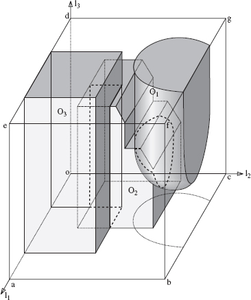
Figure 6.5 C-space and C-obstacles that correspond to W-space in Figures 6.2 and 6.4. Thicker dotted and solid lines show intersections between obstacles. Shown also are projections of the three obstacles on the plane l1, l2.
Local Directions. Similar to other algorithms in previous chapters, a common operation in the algorithm here will be the choice of a local direction for the next turn (say, left or right). This will be needed when, while moving along a curve, the C-point encounters a sort of T-intersection with another curve (which is here the horizontal part of “T”). Let us define the vector of current motion p and consider all possible cases.
- The C-point moves along the M-line or along an intersection curve between the M-plane and an obstacle and is about to leave M-plane at the cross-point. Define the normal vector m of the M-plane [97]. Then the local direction b is upward if b · m > 0 and downward if b · m ≤ 0.
- The C-point moves along the M-line or along an intersection curve between the V-plane and an obstacle, and it is about to leave V-plane at the cross-point. Let
 be the vector of l3 axis. Then, local direction b is left if
  and right if
  .
. - In a special case of motion along the M-line, the directions are
 = forward and
  = backward.
Consider the motion of a C-point in the M-plane. When, while moving along the M-line, the C-point encounters an obstacle, it may define on it a hit point, H. Here it has two choices for following the intersection curve between the M-plane and the obstacle surface: Looking from S toward T, the direction of turn at H is either left or right. We will see that sometimes the algorithm may replace the current local direction by its opposite. When, while moving along the intersection curve in the M-plane, the C-point encounters the M-line again at a certain point, it defines here the leave point, L. Similarly, when the C-point moves along a V-plane, the local directions are defined as “upward” and “downward,” where “upward” is associated with the positive and “downward”—with the negative direction of l3 axis.
6.2.2 The Approach
Similar to other cases of sensor-based motion planning considered so far, conceptually we will treat the problem at hand as one of moving a point automaton in the corresponding C-space. (This does not mean at all, as we will see, that C-space needs to be computed explicitly.) Essential in this process will be sensing information about interaction between the arm and obstacles, if any. This information—namely, what link and what part (front or rear) of the link is currently in contact with an obstacle—is obviously available only in the workspace.
Our motion planning algorithm exploits some special topological characteristics of obstacles in C-space that are a function of the arm kinematics. Note that because links l1, l2, and l3 are connected sequentially, the actual number of degrees of freedom available to them vary from link to link. For example, link l1 has only one degree of freedom: If it encounters an obstacle at some value ![]() , it simply cannot proceed any further. This means that the corresponding C-obstacle occupies all the volume of C-space that lies between the value
, it simply cannot proceed any further. This means that the corresponding C-obstacle occupies all the volume of C-space that lies between the value ![]() and one of the joint limits of joint J1. This C-obstacle thus has a simple structure: It allows the algorithm to make motion planning decisions based on the simple fact of a local contact and without resorting to any global information about the obstacle in question.
and one of the joint limits of joint J1. This C-obstacle thus has a simple structure: It allows the algorithm to make motion planning decisions based on the simple fact of a local contact and without resorting to any global information about the obstacle in question.
A similar analysis will show that C-obstacles formed by interaction between link l2 and obstacles always extend in C-space in the direction of one semi-axis of link l2 and both semi-axes of link l3; it will also show that C-obstacles formed by interaction between link l3and obstacles present generalized cylindrical holes in C-space whose axes are parallel to the axis l3. No such holes can appear, for example, along the axes l1 or l2. In other words, C-space exhibits an anisotropy property; some of its characteristics vary from one direction to the other. Furthermore, C-space possesses a certain property of monotonicity (see below), whose effect is that, no matter what the geometry of physical obstacles in W-space, no holes or cavities can appear in a C-obstacle.
From the standpoint of motion planning, the importance of these facts is in that the local information from the arm's contacts with obstacles allow one to infer some global characteristics of the corresponding C-obstacle that help avoid directions of motion leading to dead ends and thus avoid an exhaustive search.
Whereas the resulting path planning algorithm is used in the workspace, without computations of C-space, it can be conveniently sketched in terms of C-space, as follows. If the C-point meets no obstacles on its way, it will move along the M-line, and with no complications the robot will happily arrive at the target position T. If the C-point does encounter an obstacle, it will start moving along the intersection curve between the obstacle and one of the planes, M-plane or V-plane. The on-line computation of points along the intersection curve is easy: It uses the plane's equation and local information from the arm sensors.
If during this motion the C-point meets the M-line again at a point that satisfies some additional condition, it will resume its motion along the M-line. Otherwise, the C-point may arrive at an intersection between two obstacles, a position that corresponds to two links or both front and rear parts of the same link contacting obstacles. Here the C-point can choose either to move along the intersection curve between the plane and one of the obstacles, or move along the intersection curve between the two obstacles. The latter intersection curve may lead the C-point to a wall, a position that corresponds to one or more joint limits. In this case, depending on the information accumulated so far, the C-point will conclude (correctly) either that the target is not reachable or that the direction it had chosen to follow the intersection curve would lead to a dead end, in which case it will take a corrective action.
At any moment of the arm motion, the path of the C-point will be constrained to one of three types of curves, thus reducing the problem of three-dimensional motion planning to the much simpler linear planning:
- The M-line
- An intersection curve between a specially chosen plane and the surface of a C-obstacle
- An intersection curve between the surfaces of two C-obstacles
To ensure convergence, we will have to show that a finite combination of such path segments is sufficient for reaching the target position or concluding that the target cannot be reached. The resulting path presents a three-dimensional curve in C-space. No attempt will be made to reconstruct the whole or part of the space before or during the motion.
Since the path planning procedure is claimed to converge in finite time, this means that never, not even in the worst case, will the generated path amount to an exhaustive search.
An integral part of the algorithm is the basic procedure from the Bug family that we considered in Section 3.3 for two-dimensional motion planning for a point automaton. We will use, in particular, the Bug2 procedure, but any other convergent procedure can be used as well.
6.2.3 Topology of W-Obstacles and C-Obstacles
Monotonicity Property. Obstacles that intersect the W-space volume may interact with the arm during its motion. As mentioned above, one result of such interaction is the formation of obstacle shadows. Consider the spherical obstacle O1 in Figure 6.2. Clearly, no points directly above O1 can be reached by any point of the arm body. Similarly, no point of W-space below the obstacle O2 or to the left of the cubical obstacle O3 can be reached. Subsequently, the corresponding W-obstacles become as shown in Figure 6.4, and their C-space representation becomes as in Figure 6.5. This effect, studied in detail below, is caused by the constraints imposed by the arm kinematics on its interaction with obstacles. Anisotropic characteristics of W-space and C-space present themselves in a special topology of W- and C-obstacles best described by the notion of the (W- and C-) obstacle monotonicity:
Obstacle Monotonicity. In all cases of the arm interference with an obstacle, there is at least one direction corresponding to one of the axes li, i = 1, 2, 3, such that if a value ![]() of link li cannot be reached due to the interference with an obstacle, then no value
of link li cannot be reached due to the interference with an obstacle, then no value ![]() in case of contact with the link front part, or, inversely,
in case of contact with the link front part, or, inversely, ![]() in case of contact with the link rear part, can be reached either.
in case of contact with the link rear part, can be reached either.
In what follows, most of the analysis of obstacle characteristics is done in terms of C-space, although it applies to W-space as well. Comparing Figures 6.2 and 6.5, note that although physical obstacles occupy a relatively little part of the arm's workspace, their interference with the arm motion can reduce, often dramatically, the volume of points reachable by the arm end effector. The kinematic constraints are due to the arm joints, acting differently for different joint types, and to the fact that arm links are connected in series. As a result, the arm effectively has only one degree of freedom for control of motion of link l1, two degrees of freedom for control of link l2, and three degrees of freedom for control of link l3. A simple example was mentioned above on how this can affect path planning: If during the arm motion along M-line the link l1 hits an obstacle, then, clearly, the task cannot be accomplished.
The monotonicity property implies that C-obstacles, though not necessarily convex, have a very simple structure. This special topology of W- and C-obstacles will be factored into the algorithm; it allows us, based on a given local information about the arm interaction with the obstacle, to predict important properties of the (otherwise unknown) obstacle beyond the contact point. The monotonicity property can be expressed in terms more amenable to the path planning problem, as follows:
Corollary 6.2.1. No holes or cavities are possible in a C-obstacle.
W-obstacle monotonicity affects differently different links and even different parts—front or rear—of the same link. This brings about more specialized notions of li-front and li-rear monotonicity for every link, i = 1, 2, 3 (see more below). By treating links' interaction with obstacles individually and by making use of the information on what specific part—front or rear—of a given link is currently in contact with obstacles, the path planning algorithm takes advantage of the obstacle monotonicity property. Because this information is not available in C-space, the following holds:
Information Loss due to Space Transition. Information is lost in the space transition ![]() →
→ ![]() . Since some of this information—namely, the location of contact points between the robot arm and obstacles—is essential for the sensor-based planning algorithm, from time to time the algorithm may need to utilize some information specific to W-space only.
. Since some of this information—namely, the location of contact points between the robot arm and obstacles—is essential for the sensor-based planning algorithm, from time to time the algorithm may need to utilize some information specific to W-space only.
We will now consider some elemental planar interactions of arm links with obstacles, and we will show that if a path from start to target does exist, then a combination of elemental motions can produce such a path. Define the following:
- Type I obstacle corresponds to a W- or C-obstacle that results from the interaction of link l1 with a physical obstacle.
- Type II obstacle corresponds to a W- or C-obstacle that results from the interaction of link l2 with a physical obstacle.
- Type III obstacle corresponds to a W- or C-obstacle that results from the interaction of link l3with a physical obstacle.
We will use subscripts “+“ and “−“ to further distinguish between obstacles that interact with the front and rear part of a link, respectively. For example, a Type III+ obstacle refers to a C-obstacle produced by interaction of the front part of link l3 with some physical obstacle.
In the next section we will analyze separately the interaction of each link with obstacles. Each time, three cases are considered: when an obstacle interacts with the front part, the rear part, or simultaneously with both parts of the link in question. We will also consider the interaction of a combination of links with obstacles, setting the foundation for the algorithm design.
Interaction of Link l1 with Obstacles — Type I Obstacles. Since, according to our model, sliding along an obstacle does not constitute an interference with the link l1 motion, we need to consider only those cases where the link meets an obstacle head-on. When only the front end of link l1 is in contact with an obstacle—say, at the joint value ![]() —a Type I+ obstacle is produced, which extends from C-space floor to ceiling and side to side (see Figure 6.6) which effectively reduces the C-space cubicle by the volume (l1 max —
—a Type I+ obstacle is produced, which extends from C-space floor to ceiling and side to side (see Figure 6.6) which effectively reduces the C-space cubicle by the volume (l1 max — ![]() ) · l2 max · l3 max.
) · l2 max · l3 max.
A similar effect appears when only the rear end of link l1 interacts with an obstacle—say, at a joint value ![]() . Then the C-space is effectively decreased by the volume
. Then the C-space is effectively decreased by the volume ![]() · l2 max · l3 max. Finally, a simultaneous contact of both front and rear ends with obstacles at a value
· l2 max · l3 max. Finally, a simultaneous contact of both front and rear ends with obstacles at a value ![]() corresponds to a degenerate case where no motion of link l1 is possible; that is, the C-obstacle occupies the whole C-space. Formally the property of Type I obstacle monotonicity is expressed as follows:
corresponds to a degenerate case where no motion of link l1 is possible; that is, the C-obstacle occupies the whole C-space. Formally the property of Type I obstacle monotonicity is expressed as follows:
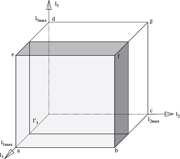
Figure 6.6 C-space with a Type I obstacle.
Type I Monotonicity. For any obstacle interacting with link l1, there are three directions corresponding to the joint axes li, i = 1, 2, 3, respectively, along which the C-obstacle behaves monotonically, as follows: If a position ![]() cannot be reached by the arm due to an obstacle interference, then no position
cannot be reached by the arm due to an obstacle interference, then no position ![]() , such that
, such that ![]() in case of the (obstacle's) contact with the link's front part, or
in case of the (obstacle's) contact with the link's front part, or ![]() in case of the contact with the link's rear part, and
in case of the contact with the link's rear part, and ![]() ,
, ![]() , can be reached either.
, can be reached either.
Interaction of Link l2 with Obstacles — Type II Obstacles
Front Part of Link l2 – Type II+ Obstacles. Consider the case when only the front part of link l2 interferes with an obstacle (Figure 6.2). Because link l2 effectively has two degrees of freedom, the corresponding Type II+ obstacle will look in C-space as shown in Figure 6.7. The monotonicity property in this case is as follows:
Type II+ Monotonicity. For any obstacle interacting with the front part of link l2, there are two axes (directions), namely l2 and l3, along which the C-obstacle behaves monotonically, as follows: If a position ![]() cannot be reached by the arm due to an obstacle interference, then no position
cannot be reached by the arm due to an obstacle interference, then no position ![]() , such that
, such that ![]() and
and ![]() , can be reached either.
, can be reached either.
As a result, a Type II+ collision, as at point H in Figure 6.7, indicates that any motion directly upward or downward from H along the obstacle will necessarily bring the C-point to one of the side walls of the C-space cubicle. This suggests that a plane can be chosen such that the exploration of the intersection curve between this plane and the Type II+ obstacle will produce a more promising outcome that will result either in a success or in the correct conclusion that the target cannot be reached. In the algorithm, the M-plane will be used, which offers some technical advantages. In general, all three arm joints will participate in the corresponding motion.
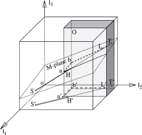
Figure 6.7 (a) W-space and (b) C-space with a Type II obstacle. (S, T) is the M-line; HabL is a part of the intersection curve between the obstacle O and M-plane.
For this case (front part of link l2 interacting with an obstacle), the decision on which local direction, right or left, is to be taken at a hit point H in order to follow the intersection curve between an M-plane and a Type II+ obstacle is made in the algorithm based on the following rule:
Rule 1:
If l1 H > l1 T, the current direction is “left.”
If l1 H > l1 T, the current direction is “right.”
If l1 H > l1 T, the target cannot be reached.
Rear Part of Link l2 – Type II_Obstacles. Now consider the case when only the rear part of link l2—that is, the link's part to the left of joint J2—can interfere with obstacles (see obstacle O3, Figure 6.2). This situation produces a C-space very similar to that in Figure 6.7. The direction of obstacle monotonicity along the axis l2 will now reverse:
Type II− Monotonicity. For any obstacle interacting with the rear part of link l2, there are two axes (directions), namely l2 and l3, along which the C-obstacle behaves monotonically, as follows: If a position ![]() cannot be reached by the arm due to an obstacle interference, then no position
cannot be reached by the arm due to an obstacle interference, then no position ![]() , such that
, such that ![]() and
and ![]() , can be reached either.
, can be reached either.
In terms of decision-making, this case is similar to the one above, except that the direction of obstacle monotonicity along l2 axis reverses, and the choice of the current local direction at a hit point H obeys a slightly different rule:
Rule 2:
If l1 H > l1 T, the current direction is “right.”
If l1 H < l1 T, the current direction is “left.”
If l1 H = l1 T, the target cannot be reached.
Interaction of Both Parts of Link l2 with Obstacles. Clearly, when both the front and the rear parts of link l2 interact simultaneously with obstacles, the resulting Type II+ and Type II− obstacles fuse into a single C-obstacle that divides C-space into two separate volumes unreachable one from another (see Figure 6.8). If going from S to T requires the arm to cross that obstacle, the algorithm will conclude that the target position cannot be reached.
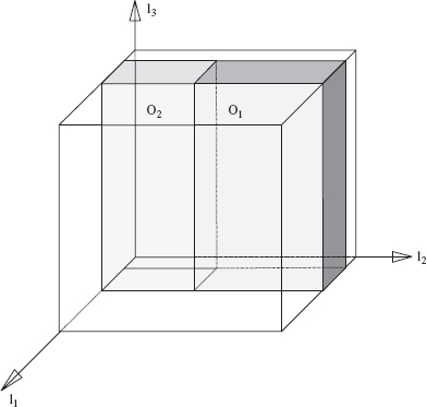
Figure 6.8 C-space in the case when both front and rear parts of link l2 interact with obstacles, producing a single obstacle that is a combination of a Type II+ and Type II− obstacles.
Front Part of Link l3 – Type III+ Obstacles. Assume for a moment that only the front part of link l3 can interfere with an obstacle (see, e.g., obstacle O1, Figures 6.2 and 6.4). Consider the cross sections of the obstacle with two horizontal planes: one corresponding to the value ![]() and the other corresponding to the value
and the other corresponding to the value ![]() with
with ![]() . Denote these cross sections a′ and a″, respectively. Each cross section is a closed set limited by a simple closed curve; it may or may not include points on the C-space boundary. Because link l3 is a generalized cylinder, the vertical projection of one cross section onto the other satisfies the relationship a′ ⊆ a″. This is a direct result of the Type III+ obstacle monotonicity property, which is formulated as follows:
. Denote these cross sections a′ and a″, respectively. Each cross section is a closed set limited by a simple closed curve; it may or may not include points on the C-space boundary. Because link l3 is a generalized cylinder, the vertical projection of one cross section onto the other satisfies the relationship a′ ⊆ a″. This is a direct result of the Type III+ obstacle monotonicity property, which is formulated as follows:
Type III+ Monotonicity. For any obstacle interacting with the front part of link l3, there is one axis (direction), namely l3, along which the corresponding C-obstacle behaves monotonically, as follows: if a position ![]() cannot be reached by the arm due to an obstacle interference, then no position
cannot be reached by the arm due to an obstacle interference, then no position ![]() such that
such that ![]() can be reached either.
can be reached either.
This property results in a special “stalactite” shape of Type III+ obstacles. A typical property of icicles and of beautiful natural stalactites that hang down from the ceilings of many caves is that their horizontal cross section is continuously reduced (in theory at least) from its top to its bottom. Each Type III+ obstacle behaves in a similar fashion. It forms a “stalactite” that hangs down from the ceiling of the C-space cubicle, and its horizontal cross section can only decrease, with its maximum horizontal cross section being at the ceiling level, l3 = l3 max(see cubicle Oabcdefg and obstacle O1, Figure 6.4). For any two horizontal cross sections of a Type III+ obstacle, taken at levels ![]() and
and ![]() such that
such that ![]() , the projection of the first cross section (
, the projection of the first cross section (![]() level) onto a horizontal plane contains no points that do not belong to the similar projection of the second cross section (
level) onto a horizontal plane contains no points that do not belong to the similar projection of the second cross section (![]() level). This behavior is the reflection of the monotonicity property.
level). This behavior is the reflection of the monotonicity property.
Because of this topology of Type III+ obstacles, the sufficient motion for maneuvering around any such obstacle—that is, motion sufficient to guarantee convergence—turns out to be motion along the intersection curves between the corresponding C-obstacle and either the M-plane or the V-plane (specifically, its part below M-plane), plus possibly some motion in the floor of the C-space cubicle (Figure 6.9).
Rear Part of Link l3 – Type III− Obstacles. A similar argument can be made for the case when only the rear end of link l3 interacts with an obstacle (see, e.g., obstacle O2, Figures 6.2, 6.4, and 6.5). In C-space the corresponding Type III− obstacle becomes a “stalagmite” growing upward from the C-space floor. This shape is a direct result of the Type III− obstacle monotonicity property, which is reversed compared to the above situation with the front part of link l3, as follows:

Figure 6.9 C-space with a Type III obstacle. (a) Curve abc is the intersection curve between the obstacle and V-plane that would be followed by the algorithm. (b) Here the Type III obstacle intersects the floor of C-space. Curve aHbLc is the intersection curve between the obstacle and V-plane and C-space floor that would be followed by the algorithm.
Type III− Monotonicity. For any obstacle interacting with the rear part of link l3, there is one axis (direction), l3, along which the corresponding C-obstacle behaves monotonically, as follows: if a position ![]() cannot be reached by the arm due to an obstacle interference, then no position
cannot be reached by the arm due to an obstacle interference, then no position ![]() such that
such that ![]() can be reached either.
can be reached either.
The motion sufficient for maneuvering around a Type III− obstacle and for guaranteeing convergence is motion along the curves of intersection between the corresponding C-obstacle and either the M-plane or the V-plane (its part above M-plane), or the ceiling of the C-space cubicle.
Interaction of Both Parts of Link l3 with Obstacles. This is the case when in C-space a “stalactite” obstacle meets a “stalagmite” obstacle and they form a single obstacle. (Again, similar shapes are found in some caves.) Then the best route around the obstacle is likely to be in the region of the “waist” of the new obstacle.
Let us consider this case in detail. For both parts of link l3 to interact with obstacles, or with different pieces of the same obstacle, the obstacles must be of both types, Type III+ and Type III−. Consider an example with two such obstacles shown in Figure 6.10. True, these C-space obstacles don't exactly look like the stalactites and stalagmites that one sees in a natural cave, but they do have their major properties: One “grows” from the floor and the other grows from the ceiling, and they both satisfy the monotonicity property, which is how we think of natural stalactites and stalagmites.
Without loss of generality, assume that at first only one part of link l3—say, the rear part—encounters an obstacle (see obstacle O2, Figure 6.10). Then the arm will start maneuvering around the obstacle following the intersection curve between the V-plane and the obstacle (path segment aH, Figure 6.10). During this motion the front part of link l3 contacts the other (or another part of the same) obstacle (here, obstacle O1, Figure 6.10).
At this moment the C-point is still in the V-plane, and also at the intersection curve between both obstacles, one of Type III+ and the other of Type III− (point H, Figure 6.10; see also the intersection curve H2cdL2fg, Figure 6.12). As with any curve, there are two possible local directions for following this intersection curve. If both of them lead to walls, then the target is not reachable. In this example the arm will follow the intersection curve—which will depart from V-plane, curve HbcL—until it meets V-plane at point L, then continue in the V-plane, and so on.
Since for the intersection between Type III+ and Type III− obstacles the monotonicity property works in the opposite directions—hence the minimum area “waist” that they form—the following statement holds (it will be used below explicitly in the algorithm):
Corollary 6.2.2. If there is a path around the union of a Type III+ and a Type III− obstacles, then there must be a path around them along their intersection curve.

Figure 6.10 C-space in the case when both front and rear parts of link l3 interact with obstacles, producing a single obstacle that is a combination of a Type III+ and Type III− obstacles.
Simultaneous Interaction of Combinations of Links with Obstacles. Since Type I obstacles are trivial from the standpoint of motion planning—they can be simply treated as walls parallel to the sides of the C-space cubicle—we focus now on the combinations of Type II and Type III obstacles. When both links l2 and l3 are simultaneously in contact with obstacles, the C-point is at the intersection curve between Type II and Type III obstacles, which presents a simple closed curve. (Refer, for example, to the intersection of obstacles O2 and O3, Figure 6.11.) Observe that the Type III monotonicity property is preserved in the union of Type II and Type III obstacles. Hence,
Corollary 6.2.3. If there is a path around the union of a Type II and a Type III obstacles, then there must be a path around them along their intersection curve.
As in the case of intersection between the Type III obstacle and the V-plane (see above), one of the two possible local directions is clearly preferable to the other. For example, when in Figure 6.11 the C-point reaches, at point b, the intersection curve between obstacles O2 and O3, it is clear from the monotonicity property that the C-point should choose the upward direction to follow the intersection curve. This is because the downward direction is known to lead to the base of the obstacle O2 “stalagmite” and is thus less promising (though not necessarily hopeless) as the upward direction (see path segments bc and cL, Figure 6.11).

Figure 6.11 The path in C-space in the presence of obstacles O2 and O3 of Figure 6.2; SHabcLdeT is the actual path of the arm endpoint, and curve S′H′a′…T′ is its projection onto the plane (l1, l2).
Let us stress that in spite of seeming multiplicity of cases and described elemental strategies, their logic is the same: All elemental strategies force the C-point to move either along the M-line, or along the intersection curves between a C-obstacle and a plane (M-plane, V-plane, or C-space side planes), or along the intersection curves between two Type III C-obstacles. Depending on the real workspace obstacles, various combinations of such path segments may occur. We will show in the next section that if in a given scene there exists a path to the target position, a combination of elemental strategies is sufficient to produce one.
6.2.4 Connectivity of 
A space or manifold is connected relative to two points in it if there is a path that connects both points and that lies fully in the space (manifold). For a given path l, the corresponding trajectory l(t) defines this path as a function of a scalar variable t; for example, t may indicate time. Denote the 2D Cartesian space formed by joint values l1, l2 as ![]() .
.
We intend to show here that for the 3D Cartesian arm the connectivity in ![]() can be deduced from the connectivity in
can be deduced from the connectivity in ![]() p. Such a relationship will mean that the problem of path planning for the 3D Cartesian arm can be reduced to that for a point automaton in the plane, and hence the planar strategies of Chapter 3 can be utilized here, likely with some modifications.
p. Such a relationship will mean that the problem of path planning for the 3D Cartesian arm can be reduced to that for a point automaton in the plane, and hence the planar strategies of Chapter 3 can be utilized here, likely with some modifications.
Define the conventional projection Pc(E) of a set of points E = {(l1, l2, l3)} ⊆ ![]() onto space
onto space ![]() p as
p as ![]() . Thus,
. Thus, ![]() c(S),
c(S), ![]() c(T),
c(T), ![]() c(M-line), and
c(M-line), and ![]() c({O}) are, respectively, the projections of points S and T, the M-line, and C-obstacles onto
c({O}) are, respectively, the projections of points S and T, the M-line, and C-obstacles onto ![]() p. See, for example, projections
p. See, for example, projections ![]() c of three obstacles, O1, O2, O3 (Figure 6.12). It is easy to see that
c of three obstacles, O1, O2, O3 (Figure 6.12). It is easy to see that ![]() c(O1 ∩ O2) =
c(O1 ∩ O2) = ![]() c(O1) ∩
c(O1) ∩ ![]() c(O2).
c(O2).
Define the minimal projection Pm(E) of a set of points E = {(l1, l2, l3)}, ⊆ ![]() onto space
onto space ![]() p as
p as ![]() m(E) = {(l1, l2) | ∀ l3, (l1, l2, l3) ∈ E}. Thus, if a C-obstacle O stretches over the whole range of l3 ∈ [0, l3 max], and E contains all the points in O, then
m(E) = {(l1, l2) | ∀ l3, (l1, l2, l3) ∈ E}. Thus, if a C-obstacle O stretches over the whole range of l3 ∈ [0, l3 max], and E contains all the points in O, then ![]() m(E) is the intersection between the (l1, l2)-space and the maximum cylinder that can be inscribed into O and whose axis is parallel to l3. Note that if a set E is a cylinder whose axis is parallel to the l3 axis, then
m(E) is the intersection between the (l1, l2)-space and the maximum cylinder that can be inscribed into O and whose axis is parallel to l3. Note that if a set E is a cylinder whose axis is parallel to the l3 axis, then ![]() c(E) =
c(E) = ![]() m(E). Type I and Type II obstacles present such cylinders. In general,
m(E). Type I and Type II obstacles present such cylinders. In general, ![]() m(S) =
m(S) = ![]() m(T) = =
m(T) = = ![]() .
.
Existence of Collision-Free Paths. We will now consider the relationship between a path in ![]() and its projection in
and its projection in ![]() p. The following statement comes directly from the definition of
p. The following statement comes directly from the definition of ![]() c and
c and ![]() m:
m:
Lemma 6.2.1. For any C-obstacle O in ![]() and any set Ep in
and any set Ep in ![]() p, if Ep ∩
p, if Ep ∩ ![]() c(O) =
c(O) = ![]() , then
, then ![]() .
.
If the hypothesis is not true, then ![]() . We have
. We have ![]()
![]() . Thus a contradiction.
. Thus a contradiction.
The next statement provides a sufficient condition for the existence of a path in C-space:
Lemma 6.2.2. Given a set of obstacles {O} in ![]() and the corresponding projections
and the corresponding projections ![]() c({O}), if there exists a path between
c({O}), if there exists a path between ![]() c(S) and
c(S) and ![]() c(T) in
c(T) in ![]() p, then there must exist a path between S and T in
p, then there must exist a path between S and T in ![]() .
.
Let lp(t) = {l1(t), l2(t)} be a trajectory of Pc(C-point) between ![]() c(S) and
c(S) and ![]() c(T) in
c(T) in ![]() p. From Lemma 6.2.1,
p. From Lemma 6.2.1, ![]() in
in ![]() . Hence, for example, the path
. Hence, for example, the path ![]() connects S and T in
connects S and T in ![]() .
.
To find the necessary condition, we will use the notion of a minimal projection. The following statement asserts that a zero overlap between two sets in ![]() implies a zero overlap between their minimal projections in
implies a zero overlap between their minimal projections in ![]() p:
p:
Lemma 6.2.3. For any set E and any C-obstacle O in ![]() , if O ∩ E =
, if O ∩ E = ![]() , then
, then ![]() m(E) ∩
m(E) ∩ ![]() m(O) =
m(O) = ![]() .
.
By definition, ![]() and
and ![]() . Thus, if
. Thus, if ![]() m(E) ∩
m(E) ∩ ![]() m(O) =
m(O) = ![]() , then
, then ![]()
![]() .
.
To use this lemma in the algorithm design, we need to describe minimal projections for different obstacle types. For any Type I or Type II obstacle O, ![]() c(O) =
c(O) = ![]() m(O). For a Type III obstacle we consider three cases, using, as an example, a Type III+ obstacle; denote it O+.
m(O). For a Type III obstacle we consider three cases, using, as an example, a Type III+ obstacle; denote it O+.
- O+ intersects the floor F of . Because of the monotonicity property,
 m(O+) = O+ ∩ F. In other words, the minimal projection of O+ is exactly the intersection area of O+ with the floor F.
 - O+ intersects with a Type III− obstacle, O−. Then, B(m(O+ ∪ O−)) = c(B(O+) ∩ B(O−)), where B(O) refers to the boundary of O. That is, the boundary curve of the combined minimal projection of O+ and O− is the conventional projection of the intersection curve between the boundary surfaces of O+ and O−.
- Neither of the above cases apply. Then m(O+) =
 .
.
A similar argument can be carried out for a Type III− obstacle.
We now turn to establishing a necessary and sufficient condition that ties the existence of paths in the plane ![]() p with that in
p with that in ![]() . This condition will provide a base for generalizing, in the next section, a planar path planning algorithm to the 3D space. Assume that points S and T lie outside of obstacles.
. This condition will provide a base for generalizing, in the next section, a planar path planning algorithm to the 3D space. Assume that points S and T lie outside of obstacles.
Theorem 6.2.1. Given points S, T and a set of obstacles {O} in ![]() , a path exists between S and T in
, a path exists between S and T in ![]() if and only if there exists a path in
if and only if there exists a path in ![]() p between points
p between points ![]() c(S) and
c(S) and ![]() c(T) among the obstacles
c(T) among the obstacles ![]() m({O}).
m({O}).
First, we prove the necessity. Let l(t), t ∈ [0, 1], be a trajectory in ![]() . From Lemma 6.2.3,
. From Lemma 6.2.3, ![]() m(l(t)) ∩
m(l(t)) ∩ ![]() m({O}) =
m({O}) = ![]() . Hence, the path
. Hence, the path ![]() m(l(t)) connects
m(l(t)) connects ![]() c(S) and
c(S) and ![]() c(T) in
c(T) in ![]() p.
p.
To show the sufficiency, let lp(t), t ∈ [0, 1], be a trajectory in ![]() p and let lp(·) be the corresponding path. Then
p and let lp(·) be the corresponding path. Then ![]() presents a manifold in
presents a manifold in ![]() . Define
. Define ![]() and let Ec be the complement of E in
and let Ec be the complement of E in ![]() . We need to show that Ec consists of one connected component. Assume that this is not true. For any t* ∈ [0, 1], since lp(t*) ∩
. We need to show that Ec consists of one connected component. Assume that this is not true. For any t* ∈ [0, 1], since lp(t*) ∩ ![]() m({O} =
m({O} = ![]() , there exists l3* such that point (lp(t*), l3*) ∈ Ec. The only possibility for Ec to consist of two or more disconnected components is when there exists t* and a set
, there exists l3* such that point (lp(t*), l3*) ∈ Ec. The only possibility for Ec to consist of two or more disconnected components is when there exists t* and a set ![]() , such that (lp(t*), l3*) ∈ E while
, such that (lp(t*), l3*) ∈ E while ![]() and
and ![]() . However, this cannot happen because of the monotonicity property of obstacles. Hence Ec must be connected, and since points S and T lie outside of obstacles, then S, T ∈ Ec. Q.E.D.
. However, this cannot happen because of the monotonicity property of obstacles. Hence Ec must be connected, and since points S and T lie outside of obstacles, then S, T ∈ Ec. Q.E.D.
Lifting 2D Algorithms into 3D Space. Theorem 6.2.1 establishes the relationship between collision-free paths in ![]() and collision-free paths in
and collision-free paths in ![]() p. We now want to develop a similar relationship between motion planning algorithms for
p. We now want to develop a similar relationship between motion planning algorithms for ![]() and those for
and those for ![]() p. We address, in particular, the following question: Given an algorithm Ap for
p. We address, in particular, the following question: Given an algorithm Ap for ![]() p, can one construct an algorithm A for
p, can one construct an algorithm A for ![]() , such that any trajectory (path) l(t) produced by A in
, such that any trajectory (path) l(t) produced by A in ![]() in the presence of obstacles {O} maps by
in the presence of obstacles {O} maps by ![]() m into the trajectory lp(t) produced by Ap in
m into the trajectory lp(t) produced by Ap in ![]() p in the presence of obstacles
p in the presence of obstacles ![]() m({O})?
m({O})?
We first define the class of algorithms from which algorithms Ap are chosen. A planar algorithm Ap is said to belong to class ![]() p if and only if its operation is based on local information, such as from tactile sensors; the paths it produces are confined to the M-line, obstacle boundaries, and W-space boundaries; and it guarantees convergence. In other words, class
p if and only if its operation is based on local information, such as from tactile sensors; the paths it produces are confined to the M-line, obstacle boundaries, and W-space boundaries; and it guarantees convergence. In other words, class ![]() p comprises only sensor-based motion planning algorithms that satisfy our usual model. In addition, we assume that all decisions about the direction to proceed along the M-line or along the obstacle boundary are made at the intersection points between M-line and obstacle boundaries.
p comprises only sensor-based motion planning algorithms that satisfy our usual model. In addition, we assume that all decisions about the direction to proceed along the M-line or along the obstacle boundary are made at the intersection points between M-line and obstacle boundaries.
Theorem 6.2.1 says that if there exists a path in ![]() p (between projections of points S and T), then there exists at least one path in
p (between projections of points S and T), then there exists at least one path in ![]() . Our goal is to dynamically construct the path in
. Our goal is to dynamically construct the path in ![]() while Ap, the given algorithm, generates its path in
while Ap, the given algorithm, generates its path in ![]() p. To this end, we will analyze five types of elemental motions that appear in
p. To this end, we will analyze five types of elemental motions that appear in ![]() , called Motion I, Motion II, Motion III, Motion IV, and Motion V, each corresponding to the
, called Motion I, Motion II, Motion III, Motion IV, and Motion V, each corresponding to the ![]() c(C-point) motion either along the
c(C-point) motion either along the ![]() c(M-line) or along the obstacle boundaries
c(M-line) or along the obstacle boundaries ![]() c({O}). Based on this analysis, we will augment the decision-making mechanism of Ap to produce the algorithm A for
c({O}). Based on this analysis, we will augment the decision-making mechanism of Ap to produce the algorithm A for ![]() .
.
Out of the three types of obstacle monotonicity property identified above, only Type III monotonicity is used in this section. One will see later that other monotonicity types can also be used, resulting in more efficient algorithms. Below, Type I and II obstacles are treated as C-space side walls; the C-space ceiling is treated as a Type III+ obstacle; and the C-space floor is treated as a Type III− obstacle. Note that when the arm comes in contact simultaneously with what it perceives as two Type III obstacles, only those of the opposite “signs” have to be distinguished—that is, a Type III+ and a Type III−. Obstacles of the same sign will be perceived as one. Below, encountering “another Type III obstacle” refers to an obstacle of the opposite sign. Then the projection ![]() m of the union of the obstacles is not zero,
m of the union of the obstacles is not zero, ![]() m(·) ≠
m(·) ≠ ![]() .
.
Among the six local directions defined in Section 6.2.1 —forward, backward, left, right, upward, and downward—the first four can be used in a 2D motion planning algorithm. Our purpose is to design a general scheme such that, given any planar algorithm Ap, a 3D algorithm A can be developed that lifts the decision-making mechanism of Ap into 3D space by complementing the set of local directions by elements upward and downward. We now turn to the study of five fundamental motions in 3D, which will be later incorporated into the 3D algorithm.
Motion I—Along the M-Line. Starting at point S, the C-point moves along the M-line, as in Figure 6.7, segment SH; this corresponds to ![]() c(C-point) moving along the
c(C-point) moving along the ![]() c(M-line) (segment S′H′, Figure 6.7). Unless algorithm Ap calls for terminating the procedure, one of these two events can take place:
c(M-line) (segment S′H′, Figure 6.7). Unless algorithm Ap calls for terminating the procedure, one of these two events can take place:
- A wall is met; this corresponds to c(C-point) encountering an obstacle. Algorithm Ap now has to decide whether c(C-point) will move along c(M-line), or turn left or right to go around the obstacle. Accordingly, the C-point will choose to reverse its local direction along the M-line, or to turn left or right to go around the wall. In the latter case we choose a path along the intersection curve between the wall and the M-plane, which combines two advantages: (i) While not true in the worst case, due to obstacle monotonicity the M-plane typically contains one of the shortest paths around the obstacle; and (ii) after passing around the obstacle, the C-point will meet the M-line exactly at the point of its intersection with the obstacle (point L, Figure 6.7), and so the path will be simpler. In general, all three joints participate in this motion.
- A Type III+ or III− obstacle is met. The C-point cannot proceed along the M-line any longer. The local objective of the arm here is to maneuver around the obstacle so as to meet the M-line again at a point that is closer to T than the encounter point. Among various ways to pass around the obstacle, we choose here motion in the V-plane. The intersection curve between the Type III obstacle and the V-plane is a simple planar curve. It follows from the monotonicity property of Type III obstacles that when the front (rear) part of link l3 hits an obstacle, then any motion upward (accordingly, downward) along the obstacle will necessarily bring the C-point to the ceiling (floor) of the C-space. Therefore, a local contact information is sufficient here for a global planning inference—that the local direction downward (upward) along the intersection curve between the V-plane and the obstacle is a promising direction. In the example in Figure 6.9a, the resulting motion produces the curve abc.
Motion II–Along the Intersection Curve Between the M-Plane and a Wall. In ![]() p, this motion corresponds to
p, this motion corresponds to ![]() c(C-point) moving around the obstacle boundary curve in the chosen direction (see Figure 6.12, segments H1aL1 and
c(C-point) moving around the obstacle boundary curve in the chosen direction (see Figure 6.12, segments H1aL1 and ![]() ). One of these two events can take place:
). One of these two events can take place:
- The M-line is encountered, as at point L1, Figure 6.12; in p this means c(M-line) is encountered. At this point, algorithm Ap will decide whether c(C-point) should start moving along the c(M-line) or continue moving along the intersection curve between the M-plane and the obstacle boundary. Accordingly, the C-point will either resume its motion along the M-line, as in Motion I, or will keep moving along the M-plane/obstacle intersection curve.
- A Type III+ or III− obstacle is met. In p, the c(C-point) keeps moving in the same local direction along the obstacle boundary (path segments bcL and b′L′, Figure 6.11). As for C-point, there are two possible directions for it to follow the intersection curve between the Type III obstacle and the wall. Since the Type III+ (or III−) monotonicity property is preserved here, the only promising local direction for passing around the Type III+ (III−) obstacle is downward (upward). This possibility corresponds to Motion IV below.

Figure 6.12 The path in C-space in the presence of obstacles O1, O2 and O3 of Figure 6.2. Trajectory SH1aL1bH2cdL2eT is the actual path of the arm endpoint; ![]() is its projection onto the plane (l1, l2).
is its projection onto the plane (l1, l2).
Motion III–Along the Intersection Curve Between the V-Plane and a Type III+ or III− Obstacle. This corresponds to moving along the ![]() c (M-line) in
c (M-line) in ![]() p. One of the following can happen:
p. One of the following can happen:
- The M-line is met. C-point resumes its motion along the M-line as in Motion I; see path segments bc, cT and b′c′, c′T′, Figure 6.9a.
- A wall is met. This corresponds to the m(C-point) encountering an obstacle. According to the algorithm Ap, c(C-point) will either reverse its local direction to move along c(M-line) or will make a turn to follow the obstacle. Accordingly, the C-point will either (a) reverse its local direction to follow the intersection curve between the V-plane and the (Type III) obstacle or (b) try to go around the union of the wall and the obstacle. For the latter motion we choose a path along the intersection curve between the wall and the Type III obstacle.
- Another Type III+ or III− obstacle is met. Since the m projection of both Type III obstacles onto p is not zero, this corresponds to the c(C-point) encountering an obstacle, which presents the m projection of the intersection curve between both obstacles. According to Ap algorithm, the c(C-point) will either (a) reverse its local direction to move along c(M-line) or (b) make a turn to follow the obstacle. Accordingly, the C-point will either (a) reverse its local direction to follow the intersection curve between V-plane and the Type III obstacle or (b) try to go around the union of two Type III obstacles. For the latter motion, we choose a path along the intersection curve between the two Type III obstacles in the local direction left or right decided by Ap.
Motion IV– Along the Intersection Curve Between a Type III Obstacle and a Wall. In ![]() p, this corresponds to the
p, this corresponds to the ![]() c(C-point) moving along the boundary of
c(C-point) moving along the boundary of ![]() m({O}); see segments bcL and b′L′, Figure 6.11. One of the following can occur:
m({O}); see segments bcL and b′L′, Figure 6.11. One of the following can occur:
- The C-point returns to the M-plane. Then C-point resumes its motion along the intersection curve between the M-plane and the wall, similar to Motion II.
- The V-plane is encountered (see point L, Figure 6.11). In p this means that c(M-line) is encountered. At this point, algorithm Ap will decide whether the c(C-point) should start moving along the c(M-line) or should continue moving along the obstacle boundary. Accordingly, the C-point will either (a) continue moving along the intersection curve between the Type III obstacle and the wall or (b) move along the intersection curve between V-plane and the Type III obstacle in the only possible local direction, as in Motion III.
- Another Type III obstacle is encountered. Then there will be a nonzero projection of the intersection curve between two Type III obstacles onto p; the c(C-point) will continue following the obstacle boundary. Accordingly, the C-point will follow the intersection curve between the two Type III obstacles in the only possible local direction, see Motion V.
Motion V — Along the Intersection Curve Between Two Type III Obstacles. In ![]() p this corresponds to the
p this corresponds to the ![]() c(C-point) moving along the boundary of
c(C-point) moving along the boundary of ![]() m({O}); see segments H2cdL2 and
m({O}); see segments H2cdL2 and ![]() , Figure 6.12. One of the following two events can occur:
, Figure 6.12. One of the following two events can occur:
- The V-plane is encountered (point L2, Figure 6.12). In p this means that c(M-line) is encountered. At this point, algorithm Ap will decide whether the c(C-point) should start moving along the c(M-line) or should continue moving along the obstacle boundary in one of the two possible directions. Accordingly, the C-point will either (a) move along the intersection curve between the V-plane and the Type III obstacle that is known to lead to the M-plane (as in Motion III.3 above) or (b) keep moving along the intersection curve between two Type III obstacles.
- A wall is encountered. In p this corresponds to continuous motion of the c(C-point) along the obstacle boundary. Accordingly, the C-point starts moving along the intersection curve between the newly encountered wall and one of the two Type III obstacles—the one that is known to lead to the M-line (as in Motion IV).
To summarize, the above analysis shows that the five motions that exhaust all distinct possible motions in ![]() can be mapped uniquely into two categories of possible motions in
can be mapped uniquely into two categories of possible motions in ![]() p—along the
p—along the ![]() c(M-line) and along
c(M-line) and along ![]() m({O})—that constitute the trajectory of the
m({O})—that constitute the trajectory of the ![]() c(C-point) in
c(C-point) in ![]() p under algorithm Ap. Furthermore, we have shown how, based on additional information on obstacle types that appear in
p under algorithm Ap. Furthermore, we have shown how, based on additional information on obstacle types that appear in ![]() , any decision by algorithm Ap in
, any decision by algorithm Ap in ![]() p can be transformed uniquely into the corresponding decision in
p can be transformed uniquely into the corresponding decision in ![]() . This results in a path in
. This results in a path in ![]() that has the same convergence characteristics as its counterpart in
that has the same convergence characteristics as its counterpart in ![]() p. Hence we have the following theorem:
p. Hence we have the following theorem:
Theorem 6.2.2. Given a planar algorithm Ap ∈ ![]() p, a 3D algorithm A can be constructed such that any trajectory produced by A in the presence of obstacles {O} in
p, a 3D algorithm A can be constructed such that any trajectory produced by A in the presence of obstacles {O} in ![]() maps by
maps by ![]() c into the trajectory that Ap produces in the presence of obstacles
c into the trajectory that Ap produces in the presence of obstacles ![]() m({O}) in
m({O}) in ![]() p.
p.
6.2.5 Algorithm
Theorem 6.2.2 states that an algorithm for sensor motion planning for the 2D Cartesian robot arm can be extended to a 3D algorithm, while preserving the algorithm's convergence. This kind of extension will not, however, necessarily produce efficient paths, since it may or may not utilize all the information available in the arm (3D) workspace. For example, the obstacle monotonicity property suggests that some directions for passing around an obstacle are more promising than others. Following the analysis in Section 6.2.4, a more efficient algorithm, which preserves the convergence properties discussed in Section 6.2.4 and also takes into account the said additional information, is presented below. The algorithm is based on a variation of the Bug2 procedure (see Section 3.3.2).
The following notation is used in the algorithm's procedure:
- Flag F is used to check whether or not both local directions have been tried for a given curve.
- Variables curr_dir and curr_loc, respectively, store the current local direction and current robot position.
- Function dist(x, y) gives the Cartesian distance between points x and y.
- Rules 1 and 2 are as defined in Section 6.2.3.
- When the C-point encounters a curve on the surface of an obstacle that it has to follow, the directions right and left are defined similar to those for the M-plane above.
- In order to choose the local direction upward or downward, function AboveMLine(curr_loc) is used to determine if the current location is above or below the M-line.
- Variable local_dir1 refers to the local directions forward, backward, left and right.
- Variable local_dir2 refers to the local directions upward and downward.
The algorithm proceeds as follows.
Step 0 Initialization. Set j = 0. Start at S. Go to Step 1.
Step 1 Motion Along the M-Line. Move along the M-line toward T until one of the following occurs:
(a) T is reached. The procedure terminates.
(b) A wall or a Type I obstacle is encountered. T cannot be reached—the procedure terminates.
(c) A Type II+ obstacle is encountered. Set j = j + 1 and define Hj = curr_loc; set F = 1 and set local_dir 1 according to Rule 1. Go to Step 2.
(d) A Type II+ obstacle is encountered. Set j = j + 1 and define Hj = curr_loc; set F = 1 and set local_dir1 according to Rule 2. Go to Step 2.
(e) A Type III obstacle is encountered. If l3 S = l3 T, T cannot be reached—the procedure terminates. Otherwise, set local_dir2 = downward or upward if the obstacle is of Type III+ (or III−); go to Step 3.
Step 2 Motion Along the Intersection Curve Between a Type II Obstacle and an M-Plane. Move along the intersection curve until one of the following occurs:
(a) The M-line is encountered. If dist(![]() c(curr_loc),
c(curr_loc), ![]() c(T)) > dist(
c(T)) > dist(![]() c(Hj),
c(Hj), ![]() c(T)), go5 to Step 2. Otherwise, define Lj = curr_loc; go to Step 1.
c(T)), go5 to Step 2. Otherwise, define Lj = curr_loc; go to Step 1.
(b) A wall or a Type I obstacle is encountered. T cannot be reached—the procedure terminates.
(c) Another Type II obstacle is encountered. T cannot be reached—the procedure terminates.
(d) A Type III obstacle is encountered. Set local_dir2 = downward or upward if the obstacle is of Type III+ (or III−). Go to Step 4.
Step 3 Motion Along the Intersection Curve Between a Type III Obstacle and a V-Plane. Move along the intersection curve until one of the following occurs:
(a) The M-line is met. Go to Step 1.
(b) A wall or a Type I obstacle is encountered. T cannot be reached—the procedure terminates.
(c) A Type II+ obstacle is encountered. Set j = j + 1 and define Hj = curr_loc; set F = 1 and set local_dir1 according to Rule 1. Go to Step 4.
(d) A Type II− obstacle is encountered. Set j = j + 1 and define Hj = curr_loc; set F = 1 and set local_dir1 according to Rule 2. Go to Step 4.
(e) Another Type III obstacle is encountered. Set j = j + 1 and define Hj = curr_loc; set F = 2 and set local_dir1 = right. Go to Step 5.
Step 4 Motion along the intersection curve between a Type II obstacle and a Type III obstacle. Move along the intersection curve until one of the following occurs:
(a) A wall or a Type I obstacle is encountered. Target T cannot be reached—the procedure terminates.
(b) The M-plane is encountered. Go to Step 2.
(c) The V-plane is encountered. If dist(![]() c(curr_loc),
c(curr_loc), ![]() c(T)) > dist(
c(T)) > dist(![]() c(Hj),
c(Hj), ![]() c(T)), then go to Step 2. Otherwise, define Lj = curr_loc; go to Step 3.
c(T)), then go to Step 2. Otherwise, define Lj = curr_loc; go to Step 3.
(d) Another Type II obstacle is encountered. Target T cannot be reached—the procedure terminates.
(e) Another Type III obstacle is encountered. Go to Step 5.
(f) The V-plane is encountered. If dist(![]() c(curr_loc),
c(curr_loc), ![]() C(T)) > dist(
C(T)) > dist(![]() c(Hj),
c(Hj), ![]() c(T)), then repeat Step 4. Otherwise, define Lj = curr_loc; go to Step 3.
c(T)), then repeat Step 4. Otherwise, define Lj = curr_loc; go to Step 3.
Step 5 Motion Along the Intersection Curve Between Two Type III Obstacles. Move along the intersection curve until one of the following occurs:
(a) A wall or a Type I obstacle is encountered. F = F − 1. If F = 0, T cannot be reached—the procedure terminates. Otherwise, set local_dir1 to its opposite; retrace to Hj; repeat Step 5.
(b) The V-plane is encountered. If dist(![]() c(curr_loc),
c(curr_loc), ![]() c(T)) > dist(
c(T)) > dist(![]() c(Hj),
c(Hj), ![]() c(T)), then repeat Step 5. Otherwise, define Lj = curr_loc; if AboveMPlane(curr_loc) = true, then follow the intersection curve between the V-plane and the Type III− obstacle. Otherwise, follow the intersection curve between the V-plane and the Type III+ obstacle. Go to Step 3.
c(T)), then repeat Step 5. Otherwise, define Lj = curr_loc; if AboveMPlane(curr_loc) = true, then follow the intersection curve between the V-plane and the Type III− obstacle. Otherwise, follow the intersection curve between the V-plane and the Type III+ obstacle. Go to Step 3.
(c) A Type II obstacle is encountered. If AboveMPlane(curr_loc) = true, then follow the intersection curve between the Type II obstacle and the Type III− obstacle. Otherwise, follow the intersection curve between the Type II obstacle and the Type III+ obstacle; go to Step 4.
6.2.6 Examples
Two examples considered here demonstrate performance of the motion planning algorithm presented in the previous section. Both examples make use of examples considered above in the course of the algorithm construction. To simplify the visualization of algorithm performance and not to overcrowd pictures with the arm links and joints, only the resulting paths are presented in Figures 6.11 and 6.12. Since for the Cartesian arm the C-space presentation of a path is the same as the path of the arm end effector in W-space, the paths are shown in C-space only.
Example 1. The arm's workspace contains only two obstacles, O2 and O3, of those three shown in Figure 6.2. Shown in Figure 6.11 are the corresponding C-obstacles, the start and target points S and T, the path (SHabcLdeT) of the arm end effector, and, for better visualization, the path's projection (S′H′…T′) onto the plane (l1, l2). Between points S and H the end effector moves in free space along the M-line. At point H the rear part of link l2 contacts obstacle O3, and the arm starts maneuvering around this (Type II) obstacle, producing path segments Ha and ab. At point b the rear part of link l3 contacts the (Type III) obstacle O2. The next two path segments, bc and cL, correspond to the motion when the arm is simultaneously in contact with both obstacles. At point L the C-point encounters the V-plane, and the next two path segments, Ld and de, correspond to the motion in the V-plane; here the arm is in contact with only one obstacle, O2. Finally, at point e the C-point encounters the M-line and the arm proceeds in free space along the M-line toward point T.
Example 2. The arm workspace here contains all three obstacles, O1, O2, and O3, of Figure 6.2. The corresponding C-space and the resulting path are shown in Figure 6.12. Up until the arm encounters obstacle O1 the path is the same as in Example 1: The robot moves along the M-line from S toward T until the rear part of link l2 contacts obstacle O3 and a hit point H1 is defined. Between points H1 and L1, the arm maneuvers around obstacle O3 by moving along the intersection curve between the M-plane and O3 and producing path segments H1 a and aL1. At point L1 the M-line is encountered, and the arm moves along the M-line toward point T until the rear part of link l3 contacts obstacle O2 at point b. Between points b and H2 the arm moves along the intersection curve between the V-plane and obstacle O2 in the direction upward. During this motion the front part of link l3 encounters obstacle O1 at the hit point H2. Now the C-point leaves the V-plane and starts moving along the intersection curve between obstacles O1 and O2 in the local direction right, producing path segments H2c, cd, and dL2. At point L2 the arm returns to the V-plane and resumes its motion in it; this produces the path segment L2e. Finally, at point e the arm encounters the M-line again and continues its unimpeded motion along the M-line toward point T.
6.3 THREE-LINK XXP ARM MANIPULATORS
In Section 6.2 we studied the problem of sensor-based motion planning for a specific type, PPP, of a three-dimensional three-link arm manipulator. The arm is one case of kinematics from the complete class XXX of arms, where each joint X is either P or R, prismatic or revolute. All three joints of arm PPP are of prismatic (sliding) type. The theory and the algorithm that we developed fits well this specific kinematic linkage, taking into account its various topological peculiarities—but it applies solely to this type. We now want to attempt a more universal strategy, for the whole group XXP of 3D manipulators, where X is, again, either P or R. As mentioned above, while this group covers only a half of the exhaustive list of XXX arms, it accounts for most of the arm types used in industry (see Figure 6.1).
As before, we specify the robot arm configuration in workspace (W-space, denoted also by ![]() ) by its joint variable vector j = (j1, j2, j3), where ji is either linear extension li for a prismatic joint, or an angle θi for a revolute joint, i = 1, 2, 3. The space formed by the joint variable vector is the arm's joint space or J-space, denoted also by
) by its joint variable vector j = (j1, j2, j3), where ji is either linear extension li for a prismatic joint, or an angle θi for a revolute joint, i = 1, 2, 3. The space formed by the joint variable vector is the arm's joint space or J-space, denoted also by ![]() . Clearly,
. Clearly, ![]() is 3D.
is 3D.
Define free J-space as the set of points in J-space that correspond to the collision-free robot arm configurations. We will show that free J-space of any XXP arm has a 2D subspace, called its deformation retract, that preserves the connectivity of the free J-space. This will allow us to reduce the problem's dimensionality. We will further show that a connectivity graph can be defined in this 2D subspace such that the existing algorithms for moving a point robot in a 2D metric space (Chapter 3) can be “lifted” into the 3D J-space to solve the motion planning problem for XXP robot arms.
In particular, in Section 6.3.1 we define the arm configuration Lj = L(j) as an image of a continuous mapping from J-space to 3D Cartesian space ℜ3, which is the connected compact set of points the arm would occupy in 3D space when its joints take the value j. A real-world obstacle is the interior of a connected compact point set in ℜ3. Joint space obstacles are thus defined as sets of points in joint space whose corresponding arm configurations have nonempty intersections with real-world obstacles. The task is to generate a continuous collision-free motion between two given start and target configurations, denoted Ls and Lt.
Analysis of a J-space in Section 6.3.2 will show that a J-space exhibits distinct topological characteristics that allow one to predict global characteristics of obstacles in ![]() based on the arm local contacts with (that is, sensing of) obstacles in the workspace. Furthermore, similar to the Cartesian arm case in Section 6.2, for all XXP arms the obstacles in
based on the arm local contacts with (that is, sensing of) obstacles in the workspace. Furthermore, similar to the Cartesian arm case in Section 6.2, for all XXP arms the obstacles in ![]() exhibit a property called the monotonicity property, as follows: For any point on the surface of the obstacle image, there exists one or more directions along which all the remaining points of
exhibit a property called the monotonicity property, as follows: For any point on the surface of the obstacle image, there exists one or more directions along which all the remaining points of ![]() belong to the obstacle. The geometric representation of this property will differ from arm to arm, but it will be there and topologically will be the same property. These topological properties bring about an important result formulated in Section 6.3.3: The free J-space,
belong to the obstacle. The geometric representation of this property will differ from arm to arm, but it will be there and topologically will be the same property. These topological properties bring about an important result formulated in Section 6.3.3: The free J-space, ![]() f, is topologically equivalent to a generalized cylinder. This result will be essential for building our motion planning algorithm.
f, is topologically equivalent to a generalized cylinder. This result will be essential for building our motion planning algorithm.
Deformation retracts ![]() of
of ![]() and
and ![]() f of
f of ![]() f, respectively, are defined in Section 6.3.4. By definition,
f, respectively, are defined in Section 6.3.4. By definition, ![]() f is a 2D surface that preserves the connectivity of
f is a 2D surface that preserves the connectivity of ![]() f. That is to say, for any two points js, jt ∈
f. That is to say, for any two points js, jt ∈ ![]() f, if there exists a path pJ ⊂
f, if there exists a path pJ ⊂ ![]() f connecting js and jt, then there must exist a path pD ⊂
f connecting js and jt, then there must exist a path pD ⊂ ![]() f connecting js and jt, and pD is topologically equivalent to pJ in
f connecting js and jt, and pD is topologically equivalent to pJ in ![]() f. Thus the dimensionality of the planning problem can be reduced.
f. Thus the dimensionality of the planning problem can be reduced.
When one or two X joints in XXP are revolute joints, X = R, ![]() is somewhat less representative of
is somewhat less representative of ![]() , only because the mapping from
, only because the mapping from ![]() to
to ![]() is not unique. That is, it may happen that L(j) = L(j′) for j ≠ j′. Let SJ = {j ∈
is not unique. That is, it may happen that L(j) = L(j′) for j ≠ j′. Let SJ = {j ∈ ![]() |L(j) = Ls} and TJ = {j ∈
|L(j) = Ls} and TJ = {j ∈ ![]() |L(j) = Lt}. The task in J-space is to find a path between any pair of points js ∈ SJ and jt ∈ TJ. We define in Section 6.3.5 a configuration space or C-space, denoted by
|L(j) = Lt}. The task in J-space is to find a path between any pair of points js ∈ SJ and jt ∈ TJ. We define in Section 6.3.5 a configuration space or C-space, denoted by ![]() , as the quotient space of
, as the quotient space of ![]() over an equivalent relation that identifies all J-space points that correspond to the same robot arm configuration. It is then shown that
over an equivalent relation that identifies all J-space points that correspond to the same robot arm configuration. It is then shown that ![]() and
and ![]() f, the quotient spaces of
f, the quotient spaces of ![]() and
and ![]() f over the same equivalent relation, are, respectively, deformation retracts of
f over the same equivalent relation, are, respectively, deformation retracts of ![]() and
and ![]() f. Therefore, the connectivity between two given robot configurations in
f. Therefore, the connectivity between two given robot configurations in ![]() can be determined in
can be determined in ![]() f.
f.
A connectivity graph ![]() will be then defined in Section 6.3.6, and it will be shown that
will be then defined in Section 6.3.6, and it will be shown that ![]() preserves the connectivity of
preserves the connectivity of ![]() f and
f and ![]() f. We will conclude that the workspace information available to the 3D robot is sufficient for it to identify and search the graph, and therefore the problem of 3D arm motion planning can be reduced to a graph search—something akin to the maze-searching problem in Chapter 3. Finally, in Section 6.3.7 we will develop a systematic approach, which, given a 2D algorithm, builds its 3D counterpart that preserves convergence.
f. We will conclude that the workspace information available to the 3D robot is sufficient for it to identify and search the graph, and therefore the problem of 3D arm motion planning can be reduced to a graph search—something akin to the maze-searching problem in Chapter 3. Finally, in Section 6.3.7 we will develop a systematic approach, which, given a 2D algorithm, builds its 3D counterpart that preserves convergence.
The following notation is used throughout this section:
- X, Y ⊂ ℜ3 are point sets.
- ∂X denotes the boundary of X.
- X ≅ Y means X is homeomorphic to Y.
 includes the closure of
 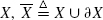 .
.- For convenience, define the closure of
 and
and 
 .
. - It is obvious that
 .
.
6.3.1 Robot Arm Representation Spaces
To recap some notations introduced earlier, a three-joint XXP robot arm manipulator is an open kinematic chain consisting of three links, Li, and three joints, Ji, i = 1, 2, 3; Ji also denotes the center point of joint Ji, defined as the intersection point between the axes of joints Ji−1 and Ji. Joints J1 and J2 can be of either prismatic (sliding) or revolute type, while joint J3 is of prismatic type. Joint J1 is attached to the base O and is the origin of the fixed reference system. Figures 6.1a–d depict XXP arm configurations. Let p denote the arm end point; θi, a revolute joint variable, li, a prismatic joint variable, and ji, either one of them, a revolute or a prismatic joint variable; i = 1, 2, 3. Figure 6.13 depicts the so-called SCARA type arm manipulator, which is of RRP type; it is arm (d) in Figure 6.1. We will later learn that from the standpoint of sensor-based motion planning the RRP arm presents the most general case among the XXP kinematic linkages.
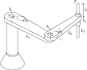
Figure 6.13 An RRP robot arm manipulator: p is the arm end point; Ji and Li are, respectively, the ith joint and link, i = 1, 2, 3; θ1, θ2, and l3 are the joint variables.
As before, assume the robot arm has enough sensing to (a) detect a contact with an approaching obstacle at any point of the robot body and (b) identify the location of that point(s) of contact on that body. The act of maneuvering around an obstacle refers to a motion during which the arm is in constant contact with the obstacle.
Without loss of generality, assume for simplicity a unit-length limit for joints, li ∈ I1 and ![]() . Points at infinity are included for convenience. The joint space
. Points at infinity are included for convenience. The joint space ![]() is defined as
is defined as ![]() , where
, where ![]() i = I1 if the ith joint is prismatic, and
i = I1 if the ith joint is prismatic, and ![]() if the ith joint is revolute. In all combinations of cases,
if the ith joint is revolute. In all combinations of cases, ![]() ≅ I3. Thus, by including points at infinity in
≅ I3. Thus, by including points at infinity in ![]() i, it is possible to treat all XXP arms largely within the same analytical framework.
i, it is possible to treat all XXP arms largely within the same analytical framework.
Definition 6.3.1. Let Lk be the set of points representing the kth robot link, k = 1, 2, 3; for any point x ∈ Lk, let x(j) ∈ ℜ3 be the point that x would occupy in ℜ3 when the arm joint vector is j ∈ ![]() . Let Lk(j) = ∪x∈ Lk x(j). Then, Lk(j) ⊂ ℜ3 is a set of points the kth robot link occupies when the arm is at j ∈
. Let Lk(j) = ∪x∈ Lk x(j). Then, Lk(j) ⊂ ℜ3 is a set of points the kth robot link occupies when the arm is at j ∈ ![]() . Similarly,
. Similarly, ![]() is a set of points the whole robot arm occupies at j ∈
is a set of points the whole robot arm occupies at j ∈ ![]() . The workspace (or W-space, denoted
. The workspace (or W-space, denoted ![]() ) is defined as
) is defined as
We assume that Li has a finite volume; thus ![]() is bounded.
is bounded.
Arm links L1 and L2 can be of arbitrary shape and dimensions. Link L3 is assumed to present a generalized cylinder —that is, a rigid body characterized by a straight-line axis coinciding with the corresponding joint axis, such that the link cross section in the plane perpendicular to the axis does not change along the axis. There are no restrictions on the shape of the cross section itself, except the physical-world assumption that it presents a simple closed curve—it can be, for example, a circle (then the link is a common cylinder), a rectangle, an oval, or any nonconvex curve.
We distinguish between the front end and rear end of link L3. The front end coincides with the arm endpoint p (see Figure 6.13). The opposite end of link L3 is its rear end. Similarly, the front (rear) part of link L3 is the part of variable length between joint J3 and the front (rear) end of link L3. Formally, we have the following definition:
Definition 6.3.2. At any given position j = (j1, j2, l3) ∈ ![]() , the front part L3+(j) of link L3 is defined as the point set
, the front part L3+(j) of link L3 is defined as the point set
![]()
Similarly, the rear part L3_(j) of link L3 is defined as the point set
![]()
The purpose of distinguishing between the front and rear parts of a prismatic (sliding) link as follows: When the front (respectively, rear) part of link L3 approaches an obstacle, the only reasonable local direction for maneuvering around the obstacle is by decreasing (respectively, increasing) the joint variable l3. This makes it easy to decide on the direction of motion based on the local contact only. Since the point set is L3((j1, j2, 0)) ∩ L3((j1, j2, 1) ⊂ L3((j1, j2, l3)) for any l3 ∈ I, and it is independent of the value of joint variable l3, the set is considered a part of L2. These definitions are easy to follow on the example of the PPP (Cartesian) arm that we considered in great detail in Section 6.2: See the arm's effective workspace in Figure 6.3a and its complete workspace in Figure 6.3b.
The robot workspace may contain obstacles. We define an obstacle as a rigid body of an arbitrary shape. Each obstacle is of finite volume (in 2D of finite area), and its surface is of finite area. Since the arm workspace is of finite volume (area), these assumptions imply that the number of obstacles present in the workspace must be finite. Being rigid bodies, obstacles cannot intersect. Formally, we have the following definition:
Definition 6.3.3. In the 2D (3D) case, an obstacle Ok, k = 1, 2, … , is the interior of a connected and compact subset of ℜ2 (ℜ3) satisfying
We use notation ![]() to represent a general obstacle, where M is the number of obstacles in
to represent a general obstacle, where M is the number of obstacles in ![]() .
.
Definition 6.3.4. The free W-space is
![]()
Lemma 6.3.1 follows from Definition 6.3.1.
Lemma 6.3.1. ![]() f is a closed set.
f is a closed set.
The robot arm can simultaneously touch more than one obstacle in the workspace. In this case the obstacles being touched effectively present one obstacle for the arm. They will present a single obstacle in the joint space.
Definition 6.3.5. An obstacle in J-space (J-obstacle) OJ ⊂ ![]() is defined as
is defined as
![]()
Theorem 6.3.1. OJ is an open set in ![]() .
.
Let j* ∈ OJ. By Definition 6.3.5, there exists a point x ∈ L such that y = x(j*) ∈ O. Since O is an open set (Definition 6.3.3), there must exist an ∈ > 0 such that the neighborhood U(y, ∈) ⊂ O. On the other hand, since x(j) is a continuous function6 from ![]() to
to ![]() , there exists a δ > 0 such that for all j ∈ U(j*, δ), we have x(j) ∈ U(y, ∈) ⊂ O; thus, U(j*, δ) ⊂ OJ, and OJ is an open set.
, there exists a δ > 0 such that for all j ∈ U(j*, δ), we have x(j) ∈ U(y, ∈) ⊂ O; thus, U(j*, δ) ⊂ OJ, and OJ is an open set.
The free J-space is ![]() . Theorem 6.3.1 gives rise to this corollary:
. Theorem 6.3.1 gives rise to this corollary:
Corollary 6.3.1. ![]() f is a closed set.
f is a closed set.
Being a closed set, ![]() . Thus, a collision-free path can pass through ∂
. Thus, a collision-free path can pass through ∂![]() f.
f.
When the arm kinematics contains a revolute joint, due to the 2π repetition in the joint position it may happen that L(j) = L(j′) for j ≠ j′. For an RR arm, for example, given two robot arm configurations, Ls and Lt, in ![]() , L(jsk1,k2) = Ls0, 0 = Ls for jsk1,k2 = (2 k1 π + θ1 s, 2 k2 π + θ2 s) ∈
, L(jsk1,k2) = Ls0, 0 = Ls for jsk1,k2 = (2 k1 π + θ1 s, 2 k2 π + θ2 s) ∈ ![]() , k1, k2 = 0, ±1, ±2, …. Similarly, L(jtk3,k4) = Lt0, 0 = Lt for jtk3,k4 = (2 k3π + θ1t, 2 k4π + θ2t) ∈
, k1, k2 = 0, ±1, ±2, …. Similarly, L(jtk3,k4) = Lt0, 0 = Lt for jtk3,k4 = (2 k3π + θ1t, 2 k4π + θ2t) ∈ ![]() , k3, k4 = 0, ±1, ±2, …. This relationship reflects the simple fact that in
, k3, k4 = 0, ±1, ±2, …. This relationship reflects the simple fact that in ![]() every link comes to exactly the same position with the periodicity 2π. In physical space this is the same position, but in J-space these are different points.7 The result is the tiling of space by tiles of size 2π. Figure 6.14 illustrates this situation in the plane. We can therefore state the motion planning task in J-space as follows:
every link comes to exactly the same position with the periodicity 2π. In physical space this is the same position, but in J-space these are different points.7 The result is the tiling of space by tiles of size 2π. Figure 6.14 illustrates this situation in the plane. We can therefore state the motion planning task in J-space as follows:
Given two robot arm configurations in ![]() , Ls and Lt, let sets
, Ls and Lt, let sets ![]() s = {j ∈
s = {j ∈ ![]() : L(j)) = Ls} and
: L(j)) = Ls} and ![]() t ={j ∈
t ={j ∈ ![]() : L(j)) = Lt} contain all the J-space points that correspond to Ls and Lt respectively. The task of motion planning is to generate a path pJ ⊂
: L(j)) = Lt} contain all the J-space points that correspond to Ls and Lt respectively. The task of motion planning is to generate a path pJ ⊂ ![]() f between js and jt for any js ∈
f between js and jt for any js ∈ ![]() s and any jt ∈
s and any jt ∈ ![]() t or, otherwise, conclude that no path exists if such is the case.
t or, otherwise, conclude that no path exists if such is the case.
The motion planning problem has thus been reduced to one of moving a point in J-space. Consider the two-dimensional RR arm shown in Figure 6.14a; shown also is an obstacle O1 in the robot workspace, along with the arm starting and target positions, S and T. Because of obstacle O1, no motion from position S to position T is possible in the “usual” sector of angles [0, 2π]. In J-space (Figure 6.14b), this motion would correspond to the straight line between points s0, 0 and t0, 0 in the square [0, 2π]; obstacle O1 appears as multiple vertical columns with the periodicity (0, 2π).
However, if no path can be found between a specific pair of positions js and jt in J-space, it does not mean that no paths between S and T exist. There may be paths between other pairs, such as between positions js0, 0 and jt1, 0 (Figure 6.14b). On the other hand, finding a collision-free path by considering all pairs of js and jt drawn from ![]() s and
s and ![]() t, respectively, is not practical because
t, respectively, is not practical because ![]() s and
s and ![]() t are likely to contain an infinite number of points. To simplify the problem further, in Section 6.3.5 we will introduce the notion of configuration space.
t are likely to contain an infinite number of points. To simplify the problem further, in Section 6.3.5 we will introduce the notion of configuration space.

Figure 6.14 The Ls and Lt configurations (positions S and T) in robot workspace in part (a) produce an infinite number of S-T pairs of points in the corresponding J-space, part (b); vertical shaded columns in J-space are J-obstacles that correspond to obstacle O1 in the robot workspace.
6.3.2 Monotonicity of Joint Space
Let Li(j) ⊂ ℜ3 be the set of points that link Li occupies when the manipulator joint value vector is j ∈ ![]() , i = 1, 2, 3 (Definition 6.3.1). Define joint space obstacles resulting from the interaction of Li with obstacle O as Type i obstacles. For link L3, let L3+ (j) and L3− (j) ⊂ ℜ3 be, respectively, the set of points that the front part and rear part of link L3 occupy when the joint value vector is j ∈
, i = 1, 2, 3 (Definition 6.3.1). Define joint space obstacles resulting from the interaction of Li with obstacle O as Type i obstacles. For link L3, let L3+ (j) and L3− (j) ⊂ ℜ3 be, respectively, the set of points that the front part and rear part of link L3 occupy when the joint value vector is j ∈ ![]() (Definition 6.3.2). Define Type 3+ and Type 3− J-obstacles respectively resulting from the interaction of L3+ and L3− with an obstacle O. More precisely:
(Definition 6.3.2). Define Type 3+ and Type 3− J-obstacles respectively resulting from the interaction of L3+ and L3− with an obstacle O. More precisely:
Definition 6.3.6. The Type i J-obstacle, i = 1, 2, 3, is defined as
Similarly, the Type 3+ and Type 3− J-obstacles are defined as
Note that OJ3 = Oj3+ ∪ OJ3− and OJ = OJ1 ∪ Oj2 ∪ OJ3. We will also need notation for the intersection of Type 3+ and Type 3− obstacles: ![]() OJ3+.
OJ3+.
We now show that the underlying kinematics of the XXP robot arm results in a special topological properties of J-space, which is best described by the notion of J-space monotonicity:
j-Space Monotonicity. In all cases of arm interference with obstacles, there is at least one of the two directions along the l3 axis, such that if a value ![]() of link L3 cannot be reached because of the interference with an obstacle, then no value
of link L3 cannot be reached because of the interference with an obstacle, then no value ![]() (in case of contact with the front part of link L3) or, inversely,
(in case of contact with the front part of link L3) or, inversely, ![]() (in case of contact with the rear part of link L3) or
(in case of contact with the rear part of link L3) or ![]() ∈ I1 (in case of contact with link L1 or L2) can be reached either.
∈ I1 (in case of contact with link L1 or L2) can be reached either.
J-space monotonicity results from the fact that link L3 of the arm manipulator presents a generalized cylinder. Because links are chained together successively, the number of degrees of freedom that a link has differs from one link to another. As a result, a specific link, or even a specific part—front or rear—of the same link can produce J-space monotonicity in one or more directions. A more detailed analysis appears further.
Lemma 6.3.2. If j = (j1, j2, l3) ∈ Oj1, ∪ Oj2, then j′ = (j1, j2, ![]() ) ∈ OJ1 ∪ OJ2 for all l3 ∈ I1.
) ∈ OJ1 ∪ OJ2 for all l3 ∈ I1.
Consider Figure 6.13. If j ∈ OJ1, then L1(j) ∩ O ≠ ![]() . Since L1(j) is independent of l3, then L1 (j′) ∩ O =
. Since L1(j) is independent of l3, then L1 (j′) ∩ O = ![]() for all j′ = (j1, j2,
for all j′ = (j1, j2, ![]() ). Similarly, if j ∈ OJ2, then L2(j) ∩ O ≠
). Similarly, if j ∈ OJ2, then L2(j) ∩ O ≠ ![]() . Since L2(j) is independent of l3, then L2(j′) ∩ O ≠
. Since L2(j) is independent of l3, then L2(j′) ∩ O ≠ ![]() for j′ = (j1, j2,
for j′ = (j1, j2, ![]() ) with any
) with any ![]() ∈ I.
∈ I.
Lemma 6.3.3. If j = (j1, j2, l3) ∈ Oj3+, then j′ = (j1, j2, ![]() ) ∈ Oj3+ for all
) ∈ Oj3+ for all ![]() > l3. If j = (j1, j2, l3) ∈ Oj3−, then j′ = (j1, j2,
> l3. If j = (j1, j2, l3) ∈ Oj3−, then j′ = (j1, j2, ![]() ) ∈ Oj3− for all
) ∈ Oj3− for all ![]() < l3.
< l3.
Using again an example in Figure 6.13, if j ∈ OJ3, then L3(j) ∩ O ≠ ![]() . Because of the linearity and the (generalized cylinder) shape of link L3, L3(j′) ∩ O ≠
. Because of the linearity and the (generalized cylinder) shape of link L3, L3(j′) ∩ O ≠ ![]() for all j′ = (j1, j2,
for all j′ = (j1, j2, ![]() ) and
) and ![]() > l3. A similar argument can be made for the second half of the lemma.
> l3. A similar argument can be made for the second half of the lemma.
Let us call the planes {l3 = 0} and {l3 = 1} the floor and ceiling of the joint space. A corollary of Lemma 6.3.3 is that if O3+ ≠ ![]() , then its intersection with the ceiling is not empty. Similarly, if O3− ≠
, then its intersection with the ceiling is not empty. Similarly, if O3− ≠ ![]() , then its intersection with the floor is nonempty. We are now ready to state the following theorem, whose proof follows from Lemmas 6.3.2 and 6.3.3.
, then its intersection with the floor is nonempty. We are now ready to state the following theorem, whose proof follows from Lemmas 6.3.2 and 6.3.3.
Theorem 6.3.2. J-obstacles exhibit the monotonicity property along the l3 axis.
This statement applies to all configurations of XXP arms. Depending on the specific configuration, though, J-space monotonicity may or may not be limited to the l3 direction. In fact, for the Cartesian arm of Figure 6.15 the monotonicity property appears along all three axes: Namely, the three physical obstacles O1, O2, and O3 shown in Figure 6.15a produce the robot workspace shown in Figure 6.15b and produce the configuration space shown in Figure 6.15c. Notice that the Type 3 obstacles O1 and O2 exhibit the monotonicity property only along the axis l3, whereas the Type 2 obstacle O3 exhibits the monotonicity property along two axes, l1 and l2. A Type 1 obstacle (not shown in the figure) exhibits the monotonicity property along all three axes (see Figure 6.6 and the related text).
6.3.3 Connectivity of  f
f
We will now show that for XXP arms the connectivity of ![]() f can be deduced from the connectivity of some planar projections of
f can be deduced from the connectivity of some planar projections of ![]() f. From the robotics standpoint, this is a powerful result: It means that the problem of path planning for a three-joint XXP arm can be reduced to the path planning for a point robot in the plane, and hence the planar strategies such as those described in Chapters 3 and 5 can be utilized, with proper modifications, for 3D planning.
f. From the robotics standpoint, this is a powerful result: It means that the problem of path planning for a three-joint XXP arm can be reduced to the path planning for a point robot in the plane, and hence the planar strategies such as those described in Chapters 3 and 5 can be utilized, with proper modifications, for 3D planning.
Let ![]() p be the floor {l3 = 0}. Clearly,
p be the floor {l3 = 0}. Clearly, ![]() . Since the third coordinate of a point in
. Since the third coordinate of a point in ![]() f is constant zero, we omit it for convenience.
f is constant zero, we omit it for convenience.
Definition 6.3.7. Given a set E = {j1, j2, l3} ⊂ ![]() , define the conventional projection Pc(E) of E onto space
, define the conventional projection Pc(E) of E onto space ![]() p as
p as ![]() .
.

Figure 6.15 The physical obstacles O1, O2, and O3 shown in figure (a) will be effectively perceived by the arm as those in figure (b), and they will produce the rather crowded C-space shown in (c).
Thus, for a joint space obstacle OJ, given start and target configurations js, jt and any path pJ between js and jt in ![]() , Pc(OJ), Pc(js), Pc(jt), and Pc(pJ) are respectively the conventional projections of OJ, js, jt, and pJ onto
, Pc(OJ), Pc(js), Pc(jt), and Pc(pJ) are respectively the conventional projections of OJ, js, jt, and pJ onto ![]() p. See, for example, the conventional projections of three obstacles, O1, O2, and O3, Figure 6.15b. It is easy to see that for any nonempty sets E1, E2 ⊂
p. See, for example, the conventional projections of three obstacles, O1, O2, and O3, Figure 6.15b. It is easy to see that for any nonempty sets E1, E2 ⊂ ![]() , we have Pc(E1 ∩ E2) = Pc(E1) ∩ Pc(E2).
, we have Pc(E1 ∩ E2) = Pc(E1) ∩ Pc(E2).
Definition 6.3.8. Define the minimal projection Pm(E) of a set of points E = {(j1, j2, l3)} ⊆ ![]() onto space
onto space ![]() p as Pm(E) = {(j1, j2)|∀l3, (j1, J2, l3) ∈ E}. For any set Ep = {j1, j2)} ⊂
p as Pm(E) = {(j1, j2)|∀l3, (j1, J2, l3) ∈ E}. For any set Ep = {j1, j2)} ⊂ ![]() p, the inverse minimal projection is
p, the inverse minimal projection is ![]()
![]() and l3 ∈ I}.
and l3 ∈ I}.
The minimal projection of a single point is empty. Hence Pm({js}) = Pm({jt}) = ![]() . If E ⊂
. If E ⊂ ![]() is homeomorphic to a sphere and stretches over the whole range of l3 ∈ I, then Pm(E) is the intersection between
is homeomorphic to a sphere and stretches over the whole range of l3 ∈ I, then Pm(E) is the intersection between ![]() p and the maximum cylinder that can be inscribed into OJ and whose axis is parallel to l3. If a set E ⊂
p and the maximum cylinder that can be inscribed into OJ and whose axis is parallel to l3. If a set E ⊂ ![]() presents a cylinder whose axis is parallel to the axis l3, then Pc(E) = Pm(E).
presents a cylinder whose axis is parallel to the axis l3, then Pc(E) = Pm(E).
In general, OJ is not homeomorphic to a sphere and may be composed of many components. We extend the notion of a cylinder as follows:
Definition 6.3.9. A subset E ⊂ ![]() presents a generalized cylinder if and only if Pc(E) = Pm(E).
presents a generalized cylinder if and only if Pc(E) = Pm(E).
Type 1 and Type 2 obstacles present such generalized cylinders. It is easy to see that for any ![]() is a generalized cylinder, and
is a generalized cylinder, and ![]()
![]() .
.
We will now consider the relationship between a path pJ in ![]() and its projection
and its projection ![]() in
in ![]() p.
p.
Lemma 6.3.4. For any set E ⊂ ![]() and any set Ep ⊂
and any set Ep ⊂ ![]() p, if Ep ∩ Pc(E) =
p, if Ep ∩ Pc(E) = ![]() , then
, then ![]() .
.
If ![]() , then we have
, then we have ![]()
![]() . Thus a contradiction.
. Thus a contradiction.
The next statement provides a sufficient condition for the existence of a path in joint space:
Lemma 6.3.5. For a given joint space obstacle OJ in ![]() and the corresponding projection Pc(OJ), if there exists a path between Pc(js) and Pc(jt) in
and the corresponding projection Pc(OJ), if there exists a path between Pc(js) and Pc(jt) in ![]() p that avoids obstacle Pc(OJ), then there must exist a path between js and jt in
p that avoids obstacle Pc(OJ), then there must exist a path between js and jt in ![]() that avoids obstacle OJ.
that avoids obstacle OJ.
Let pIp(t) = {(j1(t), j2(t))} be a path between Pc(js) and Pc(jt) in ![]() p avoiding obstacle Pc(OJ). From Lemma 6.3.4,
p avoiding obstacle Pc(OJ). From Lemma 6.3.4, ![]() in
in ![]() . Hence, for example, the path
. Hence, for example, the path ![]() connects positions js and jt in
connects positions js and jt in ![]() and avoids obstacle OJ.
and avoids obstacle OJ.
To find the necessary condition, we use the notion of a minimal projection. The next statement asserts that a zero overlap between two sets in ![]() implies a zero overlap between their minimal projections in
implies a zero overlap between their minimal projections in ![]() p:
p:
Lemma 6.3.6. For any sets E1, E2 ⊂ ![]() , if E1 ∩ E2 =
, if E1 ∩ E2 = ![]() , then Pm(E1) ∩ Pm(E2) =
, then Pm(E1) ∩ Pm(E2) = ![]() .
.
By definition, ![]() , and
, and ![]() E. Thus, if Pm(E1) ∩ Pm(E2) ≠
E. Thus, if Pm(E1) ∩ Pm(E2) ≠ ![]() , then
, then ![]()
![]() .
.
To use this lemma for designing a sensor-based motion planning algorithm, we need to describe minimal projections for different obstacle types. For a Type 1 or Type 2 obstacle O, we have Pc(O) = Pm(O). For a Type 3 obstacle, we consider three events that cover all possible cases, using as an example a Type 3+ obstacle; denote it O+.
- O+ intersects the floor f. Because of the monotonicity property, Pm(O+) = O+ ∩ f. In other words, the minimal projection of O+ is exactly the intersection area of O+ with the floor f.
- O+ intersects with a Type 3− obstacle, O−. Then, Pm(O+ ∪ O−) = Pc(∂ O+ ∩ ∂ O−). That is, the combined minimal projection of O+ and O− is the conventional projection of the intersection curve between O+ and O−.
- Neither of the above cases apply. Then Pm(O+) = .
A similar argument can be carried out for a Type 3− obstacle.
Define ![]() and
and ![]() . It is easy to see that
. It is easy to see that ![]() pf = Pc(
pf = Pc(![]() f). Therefore,
f). Therefore, ![]() .
.
Theorem 6.3.3. ![]() that is,
that is, ![]() f is topologically equivalent to a generalized cylinder.
f is topologically equivalent to a generalized cylinder.
Define ![]() . Clearly,
. Clearly, ![]() and
and ![]() . By Theorem 6.3.2, each component of
. By Theorem 6.3.2, each component of ![]() can be deformed either to the floor {l3 = 0} or to the ceiling {l3 = 1} and thus does not affect the topology of
can be deformed either to the floor {l3 = 0} or to the ceiling {l3 = 1} and thus does not affect the topology of ![]() f. Thus,
f. Thus, ![]() and, by definition,
and, by definition, ![]() presents a generalized cylinder in
presents a generalized cylinder in ![]() .
.
From the motion planning standpoint, Theorem 6.3.3 indicates that the third dimension, l3, of ![]() f is not easier to handle than the other two because
f is not easier to handle than the other two because ![]() f possesses the monotonicity property along l3 axis. It also implies that as a direct result of the monotonicity property of joint space obstacles, the connectivity of
f possesses the monotonicity property along l3 axis. It also implies that as a direct result of the monotonicity property of joint space obstacles, the connectivity of ![]() f can be decided via an analysis of 2D surfaces.
f can be decided via an analysis of 2D surfaces.
We now turn to establishing a necessary and sufficient condition that ties the existence of paths in the plane ![]() p with that in 3D joint space
p with that in 3D joint space ![]() . This condition will provide a base for generalizing planar motion planning algorithms to 3D space. Assume that points (arm positions) js and jt lie outside of obstacles.
. This condition will provide a base for generalizing planar motion planning algorithms to 3D space. Assume that points (arm positions) js and jt lie outside of obstacles.
Theorem 6.3.4. Given points js, jt ∈ ![]() f and a joint space obstacles Oj ⊂
f and a joint space obstacles Oj ⊂ ![]() , a path exists between js and jt in
, a path exists between js and jt in ![]() f if and only if there exists a path in
f if and only if there exists a path in ![]() pf between points Pc(js) and Pc(jt).
pf between points Pc(js) and Pc(jt).
To prove the necessary condition, let pJ(t), t ∈ [0, 1], be a path in ![]() f. From Lemma 6.3.6, Pm(pj(t)) ∩ Pm(Oj) =
f. From Lemma 6.3.6, Pm(pj(t)) ∩ Pm(Oj) = ![]() . Hence the path Pm(pj(t)) connects Pc(js) and Pc(jt) in
. Hence the path Pm(pj(t)) connects Pc(js) and Pc(jt) in ![]() pf.
pf.
To show the sufficiency, let pJp(t), t ∈ [0, 1], be a path in ![]() pf. Then
pf. Then ![]() presents a “wall” in
presents a “wall” in ![]() . Define
. Define ![]() and let E−1 be the complement of E in
and let E−1 be the complement of E in ![]() . We need to show that E−1 consists of one connected component. Assume that this is not true. For any t* ∈ [0, 1], since
. We need to show that E−1 consists of one connected component. Assume that this is not true. For any t* ∈ [0, 1], since ![]() , there exists l3* such that point (pJp(t*), l3*) ∈ E−1. The only possibility for E−1 to consist of two or more disconnected components is when there exists t* and a set
, there exists l3* such that point (pJp(t*), l3*) ∈ E−1. The only possibility for E−1 to consist of two or more disconnected components is when there exists t* and a set ![]() , such that (pJp(t*), l3*) ∈ E−1 while
, such that (pJp(t*), l3*) ∈ E−1 while ![]() and
and ![]() . However, this cannot happen because of the monotonicity property of obstacles. Hence E−1 must be connected.
. However, this cannot happen because of the monotonicity property of obstacles. Hence E−1 must be connected.
6.3.4 Retraction of f
Theorem 6.3.4 indicates that the connectivity of space ![]() f can indeed be captured via a space of lower dimension,
f can indeed be captured via a space of lower dimension, ![]() pf. However, space
pf. However, space ![]() pf cannot be used for motion planning because, by definition, it may happen that
pf cannot be used for motion planning because, by definition, it may happen that ![]() pf ∩ OJ ≠
pf ∩ OJ ≠ ![]() ; that is, some portion of
; that is, some portion of ![]() pf is not obstacle-free. In this section we define a 2D space
pf is not obstacle-free. In this section we define a 2D space ![]() f ⊂
f ⊂ ![]() f that is entirely obstacle-free and, like
f that is entirely obstacle-free and, like ![]() pf, captures the connectivity of
pf, captures the connectivity of ![]() f.
f.
Definition 6.3.10. [57]. A subset ![]() of a topological space χ is called a retract of χ if there exists a continuous map r: χ →
of a topological space χ is called a retract of χ if there exists a continuous map r: χ → ![]() , called a retraction, such that r(a) = a for any a ∈
, called a retraction, such that r(a) = a for any a ∈ ![]() .
.
Definition 6.3.11. [57]. A subset ![]() of space χ is a deformation retract of χ if there exists a retraction r and a continuous map
of space χ is a deformation retract of χ if there exists a retraction r and a continuous map
such that
In other words, set ![]() ⊂ χ is a deformation retract of χ if χ can be continuously deformed into A. We show below that
⊂ χ is a deformation retract of χ if χ can be continuously deformed into A. We show below that ![]() f is a deformation retract of
f is a deformation retract of ![]() f. Let
f. Let ![]() p,
p, ![]() pf, and
pf, and ![]() be as defined in the previous section; then we have the following lemma.
be as defined in the previous section; then we have the following lemma.
Lemma 6.3.7. ![]() p is a deformation retract of
p is a deformation retract of ![]() , and
, and ![]() pf is a deformation retract of
pf is a deformation retract of ![]() .
.
Define r(j1, j2, l3) = (j1, j2, 0). It follows from Lemma 6.3.2 that r is a retraction. Since for Type 1 and 2 obstacles ![]() , then, if
, then, if ![]() contains only Type 1 and Type 2 obstacles—that is,
contains only Type 1 and Type 2 obstacles—that is, ![]() f =
f = ![]() − (OJ1 ∪ OJ2)—it follows that
− (OJ1 ∪ OJ2)—it follows that ![]() and
and ![]() pf is a deformation retract of
pf is a deformation retract of ![]() f. In the general case, all obstacle types (including Type 3) can be present, and
f. In the general case, all obstacle types (including Type 3) can be present, and ![]() pf is not necessarily a deformation retract of
pf is not necessarily a deformation retract of ![]() f.
f.
Theorem 6.3.5. Let ![]() , and
, and ![]() . Then,
. Then,
![]()
is a deformation retract of ![]() f.
f.
![]() 1 and
1 and ![]() 2, are respectively, the obstacle-free portion of ∂ OJ3− and
2, are respectively, the obstacle-free portion of ∂ OJ3− and ![]() p. It is easy to see that
p. It is easy to see that ![]() f ≅
f ≅ ![]() pf. Since
pf. Since ![]() (Theorem 6.3.3) and
(Theorem 6.3.3) and ![]() pf is a deformation retract of
pf is a deformation retract of ![]() (Lemma 6.3.7), then
(Lemma 6.3.7), then ![]() f is a deformation retract of
f is a deformation retract of ![]() f.
f.
Let ![]() denote the 2D space obtained by patching all the “holes” in
denote the 2D space obtained by patching all the “holes” in ![]() f so that
f so that ![]() ≅
≅ ![]() p. It is obvious that
p. It is obvious that ![]() is a deformation retract of
is a deformation retract of ![]() .
.
Theorem 6.3.6. Given two points ![]() , if there exists a path pJ ⊂
, if there exists a path pJ ⊂ ![]() f connecting
f connecting ![]() and
and ![]() , then there exists a path pD ⊂
, then there exists a path pD ⊂ ![]() f, such that pD ∼ pJ.
f, such that pD ∼ pJ.
From Theorem 6.3.5, ![]() f is a deformation retract of
f is a deformation retract of ![]() f. Let r be the retraction as in Ref. 57, II.4; then p′ = r(p) must be an equivalent path in
f. Let r be the retraction as in Ref. 57, II.4; then p′ = r(p) must be an equivalent path in ![]() f.
f.
On the other hand, if ![]() and
and ![]() are not connected in
are not connected in ![]() f, then by definition
f, then by definition ![]() and
and ![]() are not connected in
are not connected in ![]() f either. Hence the connectivity of
f either. Hence the connectivity of ![]() and
and ![]() can be determined completely by studying
can be determined completely by studying ![]() f, which is simpler than
f, which is simpler than ![]() f because the dimensionality of
f because the dimensionality of ![]() f is lower than that of
f is lower than that of ![]() f. Furthermore, a path between two given points js = (j1s, j2s, l3s), jt = (j1t, j2t, l3t) ∈
f. Furthermore, a path between two given points js = (j1s, j2s, l3s), jt = (j1t, j2t, l3t) ∈ ![]() f can be obtained by finding the path between the two points
f can be obtained by finding the path between the two points ![]()
![]() f. Because of the monotonicity property (Theorem 6.3.2),
f. Because of the monotonicity property (Theorem 6.3.2), ![]() and
and ![]() always exist and they can be respectively connected within
always exist and they can be respectively connected within ![]() f with js and jt via vertical line segments. Hence the following statement:
f with js and jt via vertical line segments. Hence the following statement:
Corollary 6.3.2. The problem of finding a path in the 3D subset ![]() f between points js, jt ∈
f between points js, jt ∈ ![]() f can be reduced to one of finding a path in its 2D subset
f can be reduced to one of finding a path in its 2D subset ![]() f.
f.
6.3.5 Configuration Space and Its Retract
Our motion planning problem has thus been reduced to one of moving a point in a 2D subset of J-space, ![]() . However, as pointed out in Section 6.3.1, the joint space
. However, as pointed out in Section 6.3.1, the joint space ![]() is not very representative when revolute joints are involved, because the mapping from
is not very representative when revolute joints are involved, because the mapping from ![]() to workspace
to workspace ![]() is not unique. Instead, we define configuration space
is not unique. Instead, we define configuration space ![]() :
:
Definition 6.3.12. Define an equivalence relation ![]() in
in ![]() as follows: for j = (j1, j2, jw),
as follows: for j = (j1, j2, jw), ![]() if and only if (ji −
if and only if (ji − ![]() )%2π = 0, for i = 1, 2, 3, where % is the modular operation. The quotient space
)%2π = 0, for i = 1, 2, 3, where % is the modular operation. The quotient space ![]() is called the configuration space (C-space), with normal quotient space topology assigned, see Ref. 57, A.1. Let c =
is called the configuration space (C-space), with normal quotient space topology assigned, see Ref. 57, A.1. Let c = ![]() j represent an equivalence class; then the project f :
j represent an equivalence class; then the project f : ![]() →
→ ![]() is given by f(j) =
is given by f(j) = ![]() j.
j.
Theorem 6.3.7. The configuration space ![]() is compact and of finite volume (area).
is compact and of finite volume (area).
By definition, ![]() . Define equivalence relations
. Define equivalence relations ![]() i in
i in ![]() i such that
i such that ![]() if and only if
if and only if ![]() . Define
. Define ![]() and the project fi :
and the project fi : ![]() i →
i → ![]() i given by fi(j) =
i given by fi(j) = ![]() ij. Apparently,
ij. Apparently, ![]() i ≅ S1 with length υi = 2π if
i ≅ S1 with length υi = 2π if ![]() i =
i = ![]() , and
, and ![]() i ≅ I1 with length υi = 1 if
i ≅ I1 with length υi = 1 if ![]() i = I1. Because f is the product of fi's, fi's are both open and closed, and the product topology and the quotient topology on
i = I1. Because f is the product of fi's, fi's are both open and closed, and the product topology and the quotient topology on ![]() 1 ×
1 × ![]() 2 ×
2 × ![]() 3 are the same (see Ref. 57, Proposition A.3.1); therefore,
3 are the same (see Ref. 57, Proposition A.3.1); therefore, ![]() ≅
≅ ![]() 1 ×
1 × ![]() 2 ×
2 × ![]() 3 is of finite volume υ1 · υ2 · υn.
3 is of finite volume υ1 · υ2 · υn.
For an RR arm, for example, ![]() ≅ S1 × S1 with area 2π · 2π = 4π2; for an RRP arm,
≅ S1 × S1 with area 2π · 2π = 4π2; for an RRP arm, ![]() ≅ S1 × S1 × I1 with volume 2π · 2π · 1 = 4π2.
≅ S1 × S1 × I1 with volume 2π · 2π · 1 = 4π2.
For c ∈ ![]() , we define
, we define ![]() , where j ∈ f−1(c), to be the area the robot arm occupies in
, where j ∈ f−1(c), to be the area the robot arm occupies in ![]() when its joint vector is j.
when its joint vector is j.
Definition 6.3.13. The configuration space obstacle (C-obstacle) is defined as
![]()
The free C-space is ![]() .
.
The proof for the following theorem and its corollary are analogous to those for Theorem 6.3.1.
Theorem 6.3.8. A C-obstacle is an open set.
Corollary 6.3.3. The free C-space ![]() f is a closed set.
f is a closed set.
The configuration space obstacle OC may have more than one component. For convenience, we may call each component an obstacle.
Theorem 6.3.9. Let L(cs) = Ls and L(ct) = Lt. If there exists a collision-free path (motion) between Ls and Lt in ![]() , then there is a path pC ⊂
, then there is a path pC ⊂ ![]() f connecting cs and ct, and vice versa.
f connecting cs and ct, and vice versa.
If there exists a motion between Ls and Lt in ![]() , then there must be a path pJ ⊂
, then there must be a path pJ ⊂ ![]() f between two points js, jt ∈
f between two points js, jt ∈ ![]() f such that L(js) = Ls and L(jt) = Lt. Then, pC = f(pJ) ⊂
f such that L(js) = Ls and L(jt) = Lt. Then, pC = f(pJ) ⊂ ![]() f is a path between
f is a path between ![]() s = f(js) and ct = f(jt). The other half of the theorem follows directly from the definition of
s = f(js) and ct = f(jt). The other half of the theorem follows directly from the definition of ![]() f.
f.
We have thus reduced the motion planning problem in the arm workspace to the one of moving a point from start to target position in C-space.
The following characteristics of the C-space topology of XXP arms are direct results of Theorem 6.3.7:
- For a PPP arm, ≅ I1 × I1 × I1, the unit cube.
- For a PRP or RPP arm, ≅ S1 × I1 × I1, a pipe.
- For an RRP arm, ≅ S1 × S1 × I1, a solid torus.
Figure 6.16 shows the C-space of an RRP arm, which can be viewed either as a cube with its front and back, left and right sides pairwise identified, or as a solid torus.
The obstacle monotonicity property is preserved in configuration space. This is simply because the equivalent relation that defines ![]() and
and ![]() f from
f from ![]() and
and ![]() f has no effect on the third joint axis, l3. Thus we have the following statement:
f has no effect on the third joint axis, l3. Thus we have the following statement:
Theorem 6.3.10. The configuration space obstacle OC possesses the monotonicity property along l3 axis.
As with the subset ![]() f,
f, ![]() p ⊂
p ⊂ ![]() can be defined as the set {l3 = 0}; OC1, OC2, OC3, OC3+, OC3_, Pc, Pm,
can be defined as the set {l3 = 0}; OC1, OC2, OC3, OC3+, OC3_, Pc, Pm, ![]() f,
f, ![]() pf, and
pf, and ![]() can be defined accordingly.
can be defined accordingly.
Theorem 6.3.11. Let ![]() and
and ![]() . Then,
. Then,
![]()
is a deformation retract of ![]() f.
f.
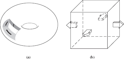
Figure 6.16 Two views of C-space of an RRP arm manipulator: (a) As a unit cube with its front and back, left and right sides pairwise identified; and (b) as a solid torus.
The proof is analogous to that of Theorem 6.3.5. Let ![]() denote the 2D space obtained by patching all the “holes” in
denote the 2D space obtained by patching all the “holes” in ![]() f so that
f so that ![]() ≅
≅ ![]() p. It is obvious that
p. It is obvious that ![]() ≅
≅ ![]() p ≅
p ≅ ![]() is a deformation retract of
is a deformation retract of ![]() . We obtain the following statement parallel to Theorem 6.3.6.
. We obtain the following statement parallel to Theorem 6.3.6.
Theorem 6.3.12. Given two points ![]() ,
, ![]() ∈
∈ ![]() f, if there exists a path pC ⊂
f, if there exists a path pC ⊂ ![]() f connecting
f connecting ![]() and
and ![]() , then there must exist a path pB ⊂
, then there must exist a path pB ⊂ ![]() f, such that pB ∼ PJ.
f, such that pB ∼ PJ.
A path between two given points js = (j1s, j2s, l3s), jt = (j1t, j2t, l3t) ∈ ![]() f can be obtained by finding the path between the two points
f can be obtained by finding the path between the two points ![]() ,
, ![]() . Because of the monotonicity property (Theorem 6.3.10),
. Because of the monotonicity property (Theorem 6.3.10), ![]() and
and ![]() always exist and can be respectively connected within
always exist and can be respectively connected within ![]() f with js and jt via vertical line segments. Hence the following statement:
f with js and jt via vertical line segments. Hence the following statement:
Corollary 6.3.4. The problem of finding a path in ![]() f between points js, jt ∈
f between points js, jt ∈ ![]() f can be reduced to that of finding a path in its subset
f can be reduced to that of finding a path in its subset ![]() f.
f.
6.3.6 Connectivity Graph
At this point we have reduced the problem of motion planning for an XXP arm in 3D space to the study of a 2D subspace ![]() that is homeomorphic to a common torus.
that is homeomorphic to a common torus.
Consider the problem of moving a point on a torus whose surface is populated with obstacles, each bounded by simple closed curves. The torus can be represented as a square with its opposite sides identified in pairs (see Figure 6.17a). Note that the four corners are identified as a single point. Without loss of generality, let the start and target points S and T be respectively in the center and the corners of the square. This produces four straight lines connecting S and T, each connecting the center of the square with one of its corners. We call each line a generic path and denote it by gi, i = 1, 2, 3, 4.
Define a connectivity graph ![]() on the torus by the obstacle-free portions of any three of the four generic paths and the obstacle boundary curves. We have the following statement:
on the torus by the obstacle-free portions of any three of the four generic paths and the obstacle boundary curves. We have the following statement:
Theorem 6.3.13. On a torus, if there exists an obstacle-free path connecting two points S and T, then there must exist such a path in the connectivity graph ![]() .
.
Without loss of generality, let g1, g2, and g3 be the complete set of generic paths, as shown in Figure 6.17a, where the torus is represented as a unit square with its opposite sides identified.
The generic paths g1, g2, and g3 cut the unit square into three triangular pieces. Rearrange the placements of the three pieces by identifying the opposite sides of the square in pairs along edges a and b, respectively (see Figures 6.17b and 6.17c). We thus obtain a six-gon (hexagon), with three pairs of S and T as its vertices and generic paths g1, g2, and g3 as its edges. The hexagon presentation is called the generic form of a torus.
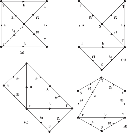
Figure 6.17 Paths g1, g2, and g3 constitute a complete set of generic paths. A hexagon is obtained by (a) cutting the square along g1, g2, and g3, (b) pasting along b, and (c) pasting along a. (d) The resulting hexagon.
Now consider the effects of the above operation on obstacles (see Figure 6.18a). Obstacle boundaries and the generic paths partition our hexagon into occupied areas (shaded areas in Figure 6.18b) and free areas (numbered I, II, III, IV and V in Figure 6.18b). Each free area is not necessarily simple, but it must be homeomorphic to a disc, possibly with one or more smaller discs removed (e.g., area I of Figure 6.18b has the disc that corresponds to obstacle O2 removed). The free area's inner boundaries are formed by obstacle boundaries; its outer boundary consists of segments of obstacle boundaries and segments of the generic paths.
Any arbitrary obstacle-free path p that connects points S and T consists of one or more segments, p1, p2, …, pn, in the hexagon. Let xi, yi be the end points of segment pi, where x1 = S, xi+1 = yi for i = 1, 2, … , n − 1, and yn = T. Since p is obstacle-free, xi and yi must be on the outer boundary of the free area that contains pi. Therefore, xi and yi can be connected by a path segment ![]() of the outer boundary of the free area. The path
of the outer boundary of the free area. The path ![]() that connects S and T and consists of segments of the generic paths and segments of obstacle boundaries is therefore entirely on the connectivity graph
that connects S and T and consists of segments of the generic paths and segments of obstacle boundaries is therefore entirely on the connectivity graph ![]() .
.
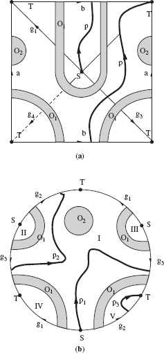
Figure 6.18 Illustration for Theorem 6.3.13. Shown are two obstacles O1, O2 (shaded areas) and path p (thicker line). The torus is represented, respectively, as (a) a unit square with its opposite sides a and b identified in pairs and (b) as a hexagon, with generic paths as its sides. Segments p1, p2 and p3 in (b) are connected; they together correspond to the path p in (a).
Figure 6.18a presents a torus shown as a unit square, with its opposite sides a and b identified in pairs. O1 and O2 are two obstacles. Note that the three pieces of obstacle O1 in the figure are actually connected. Segments g1, g2 and g3 are (any) three of the four generic paths.
For an XXP arm, we now define generic paths and the connectivity graph in ![]() , which is homeomorphic to a torus.
, which is homeomorphic to a torus.
Definition 6.3.14. For any two points a, b ∈ ![]() , let
, let ![]() be the straight line segment connecting a and b. A vertical plane is defined as
be the straight line segment connecting a and b. A vertical plane is defined as
![]()
where Pc and Pm are respectively the conventional and minimal projections as in Definition 6.3.7 and Definition 6.3.8.
In other words, ![]() ab contains both a and b and is parallel to the l3 axis. The degenerate case where
ab contains both a and b and is parallel to the l3 axis. The degenerate case where ![]() is parallel to the l3 axis is simple to handle and is not considered.
is parallel to the l3 axis is simple to handle and is not considered.
Definition 6.3.15. Let Ls and Lt be the given start and target configurations of the arm, and let ![]() and
and ![]() , respectively, be the sets of points corresponding to Ls and Lt. Let f:
, respectively, be the sets of points corresponding to Ls and Lt. Let f: ![]() →
→ ![]() be the projection as in Definition 6.3.12. Then the vertical surface
be the projection as in Definition 6.3.12. Then the vertical surface ![]() ⊂
⊂ ![]() is defined as
is defined as
![]()
For the RRP arm, which is the most general case among XXP arms, ![]() consists of four components
consists of four components ![]() i, i = 1, 2, 3, 4. Each
i, i = 1, 2, 3, 4. Each ![]() i represents a class of vertical planes in
i represents a class of vertical planes in ![]() and can be determined by the first two coordinates of a pair of points drawn respectively from
and can be determined by the first two coordinates of a pair of points drawn respectively from ![]() and
and ![]() . If
. If ![]() and
and ![]() are the robot's start and target configurations, the four components of the vertical surface
are the robot's start and target configurations, the four components of the vertical surface ![]() can be represented as follows:
can be represented as follows:
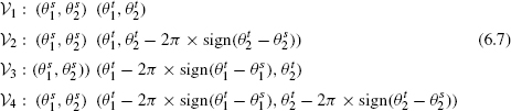
where sign() takes the values +1 or −1 depending on its argument. Each of the components of V-surface determines a generic path, as follows:
![]()
Since ![]() is homeomorphic to a torus, any three of the four generic paths can be used to form a connectivity graph. Without loss of generality, let
is homeomorphic to a torus, any three of the four generic paths can be used to form a connectivity graph. Without loss of generality, let ![]() and denote
and denote ![]() . A connectivity graph can be defined as
. A connectivity graph can be defined as ![]() . If there exists a path in
. If there exists a path in ![]() f, then at least one such path can be found in the connectivity graph
f, then at least one such path can be found in the connectivity graph ![]() .
.
Now we give a physical interpretation of the connectivity graph ![]() ;
; ![]() consists of the following curves:
consists of the following curves:
- ∂p—the boundary curve of the floor, identified by the fact that the third link of the robot reaches its lower joint limit (l3 = 0) and, simultaneously, one or both of the other two links reach their joint limits.
- p ∩ ∂(OC1 ∪ OC2)—the intersection curve between the floor and the Type 1 or Type 2 obstacle boundary, identified by the fact that the third link of the robot reaches its lower joint limit (l3 = 0) and simultaneously, one or both of the other two links contact some obstacles.
- ∂ OC3− ∩ ∂ —the intersection curve between the Type 3− obstacle boundary and C-space boundary, identified by the fact that the robot's third link touches obstacles with its rear part and, simultaneously, one or more links reach their joint limits; this case includes the intersection curve between a Type 3− obstacle boundary and the ceiling.
- ∂ OC3− ∩ ∂(OC1 ∪ OC2)—the intersection curve between the Type 3− obstacle boundary and the Type 1 or Type 2 obstacle boundary, identified by the fact that the third link of the robot touches obstacles with its rear part and that, simultaneously, one or both of the other two links contact some obstacles.
- ∂ OC3− ∩ ∂ OC3+—the intersection curve between the Type 3+ obstacle boundary and the Type 3− obstacle boundaries, identified by the fact that both front and rear parts of the third link contact obstacles.
- g ∩ pf —the obstacle-free portion of the generic path, identified by the fact that the robot is on the V-surface and that the third joint reaches its lower limit (l3 = 0).
 ∩ ∂ OC3− —the intersection curve between V-surface and the Type 3− obstacle boundaries, identified by the fact that the robot is on V-surface and simultaneously touches the obstacle with the rear part of its third link.
Note that the sensing capability of the robot arm manipulator allows it to easily identify the fact of being at any of the curves above.
6.3.7 Lifting 2D Algorithms into 3D
We have reduced the problem of motion planning for an XXP arm to the search on a connectivity graph. The search itself can be done using any existing graph search algorithm. The efficiency of a graph search algorithm is often in general—and, as we discussed above, in the Piano Mover's approach in particular—measured by the total number of nodes visited and the number of times each node is visited, regardless of the number of times that each edge is visited. In robotics, however, what is important is the total number of edge traverses, because physically each edge presents a part of the path whose length the robot may have to pass. For this reason, typical graph algorithms—for example, the width-first search algorithm [114]—would be inefficient from the standpoint of robot motion planning. On the other hand, depth-first search algorithms may work better; Tarry's rule [42] and Fraenkel's rule [45], which we discussed in Section 2.9.1, are two versions of such search algorithms. More efficient algorithms can be obtained by taking into account specifics of the connectivity graph topology [59].
In this section we intend to show how a 2D motion planning algorithm—we will call it Ap —can be carried out in ![]() f. We assume that Ap operates according to our usual model—that is, using local information from the robot tactile sensors, the paths it produces are confined to generic paths, obstacle boundaries, and space boundaries, if any—and that it guarantees convergence.8 As before, it is also assumed that all decisions as to what directions the robot will follow along the generic path or along an obstacle boundary are made at the corresponding intersection points.
f. We assume that Ap operates according to our usual model—that is, using local information from the robot tactile sensors, the paths it produces are confined to generic paths, obstacle boundaries, and space boundaries, if any—and that it guarantees convergence.8 As before, it is also assumed that all decisions as to what directions the robot will follow along the generic path or along an obstacle boundary are made at the corresponding intersection points.
Without loss of generality, side walls of the C-space, if any, are simply treated below as Type I and Type II obstacles, the C-space ceiling is treated as a Type III+ obstacle, and the C-space floor is treated as a Type III− obstacle.
Since the robot start and target positions are not necessarily in ![]() f, our first step is to bring the robot to
f, our first step is to bring the robot to ![]() f. This is easily achieved by moving from js downward until a Type III− obstacle is encountered; that is, the link L3 of the robot either reaches its joint limit or touches an obstacle with its rear end. Then, the robot switches to Ap, which searches for point
f. This is easily achieved by moving from js downward until a Type III− obstacle is encountered; that is, the link L3 of the robot either reaches its joint limit or touches an obstacle with its rear end. Then, the robot switches to Ap, which searches for point ![]() directly above or below jt, with the following identification of path elements:
directly above or below jt, with the following identification of path elements:
- Generic path—the intersection curve of and ∂ O3−.
- Obstacle boundary—the intersection curve of ∂ O3− and ∂(O1 ∪ O2 ∪ O3+).
If Ap terminates without reaching ![]() , then the target jt is not reachable. On the other hand, if
, then the target jt is not reachable. On the other hand, if ![]() is reached, then the robot moves directly toward jt. Along this path segment the robot will either reach jt or encounter an obstacle, in which case the target is not reachable. This shows how a motion planning algorithm for a compact 2D surface can be “lifted” into 3D to solve the motion planning problem of an XXP arm.
is reached, then the robot moves directly toward jt. Along this path segment the robot will either reach jt or encounter an obstacle, in which case the target is not reachable. This shows how a motion planning algorithm for a compact 2D surface can be “lifted” into 3D to solve the motion planning problem of an XXP arm.
6.3.8 Step Planning
Similar to 2D algorithms in Chapter 5, realization of the above 3D motion planning algorithms requires a complementary lower-level control piece for step calculation. The required procedure for step calculation is similar to the one sketched in Section 5.2.3 for a 2D arm, except here the tangent to the C-obstacle at the local point of contact is three-dimensional. Since, according to the motion planning algorithm, the direction of motion is always unique—the curve along which the arm moves is either an M-line, or an intersection curve between an obstacle and one of the planes M-plane or V-plane, or an intersection curve between obstacles—the tangent to the C-obstacle at the contact point is unique as well. More detail on the step calculation procedure can be found in Refs. 106 and 115.
6.3.9 Discussion
As demonstrated in this section, the kinematic constraints of any XXP arm major linkage result in a certain property—called monotonicity—of the arm joint space and configuration space (C-space or ![]() f). The essence of the monotonicity property is that for any point on the surface of a C-space obstacle, there exists at least one direction in C-space that corresponds to one of the joint axes, such that no other points in space along this direction can be reached by the arm. The monotonicity property allows the arm to infer some global information about obstacles based on local sensory data. It thus becomes an important component in sensor-based motion planning algorithms. We concluded that motion planning for a three-dimensional XXP arm can be done on a 2D compact surface,
f). The essence of the monotonicity property is that for any point on the surface of a C-space obstacle, there exists at least one direction in C-space that corresponds to one of the joint axes, such that no other points in space along this direction can be reached by the arm. The monotonicity property allows the arm to infer some global information about obstacles based on local sensory data. It thus becomes an important component in sensor-based motion planning algorithms. We concluded that motion planning for a three-dimensional XXP arm can be done on a 2D compact surface, ![]() f, which presents a deformation retract of the free configuration space
f, which presents a deformation retract of the free configuration space ![]() f.
f.
We have further shown that any convergent 2D motion planning algorithm for moving a point on a compact surface (torus, in particular) can be “lifted” into 3D for motion planning for three-joint XXP robot arms. The strategy is based on the monotonicity properties of C-space.
Given the arm's start and target points js, jt ∈ ![]() f and the notions “above” and “below” as defined in this section, the general motion planning strategy for an XXP arm can be summarized as consisting of these three steps:
f and the notions “above” and “below” as defined in this section, the general motion planning strategy for an XXP arm can be summarized as consisting of these three steps:
- Move from js to
 , where ∈
  f is directly above or below js;
 - find a path between and
 within f, where ∈ f is directly above or below jt; and
 - move from to jt.
Because of the monotonicity property, motion in Steps 1 and 3 can be achieved via straight line segments. In reality, Step 2 does not have to be limited to the plane: It can be “lifted” into 3D by modifying the 2D algorithm respectively, thus resulting in local optimization and shorter paths. With the presented theory, and with various specific algorithms presented in this and previous chapters, one should have no difficulty constructing one's own sensor-based motion planning algorithms for specific XXP arm manipulators.
6.4 OTHER XXX ARMS
One question about motion planning for 3D arm manipulators that still remains unanswered in this chapter is, How can one carry out sensor-based motion planning for XXR arm manipulators—that is, arms whose third joint is of revolute type? At this time, no algorithms with a solid theoretical foundation and with guaranteed convergence can be offered for this group. This exciting area of research, of much theoretical as well as practical importance, still awaits for its courageous explorers.
In engineering terms, one kinematic linkage from the XXR group, namely RRR, is of much importance among industrial robot manipulators. On a better side, the RRR linkage is only one out of the five 3D linkages shown in Figure 6.1, Section 6.1, which together comprise the overwhelming majority of robot arm manipulators that one finds in practice. Still, RRR is a popular arm, and knowing how to do sensor-based motion planning for it would be of much interest. Judging by our analysis of the RR arm in Chapter 5, it is also likely the most difficult arm for sensor-based motion planning.
Conceptually, the difficulty with the RRR arm, and to some extent with other XXR arms, is of the same kind that we discussed in the Section 6.1, when describing a fly moving around an object in three-dimensional space. The fly has an infinite number of ways to go around the object. Theoretically, it may need to try all those ways in order to guarantee getting “on the other side” of the object.
We have shown in this chapter that, thanks to special properties of monotonicity of the corresponding configuration space, no infinite motion will ever be necessary for any XXP arm manipulator in order to guarantee convergence. No matter how complex are the 3D objects in the arm's workspace, the motion planning algorithm guarantees a finite (and usually quick) path solution. No such properties have been found so far for the XXR arm manipulators. On the other hand, similar to XXP arms considered in this chapter, motion planning for XXR arms seems to be reducible to motion along curves that are similar to curves we have used for XXP algorithms (such as an intersection curve between an obstacle and an M-plane or V-plane, etc.). Even in the worst case, this would require a search of a relatively small graph.
Provided that the arm has the right whole-body sensing, in practice one can handle an XXR arm by using the motion planning schemes developed in this chapter for XXP arms, perhaps with some heuristic modifications. Some such attempts, including physical experiments with industrial RRR arm manipulators, are in described Chapter 8 (see also Ref. 115).
1One may argue that the fly can use its vision to space its loops far enough from each other, making the whole exercise quite doable. This may be true, but not so in general: The room may be dark, or the obstacle may be terribly wrinkled, with caves and overhangs and other hooks and crannies so that the fly's vision will be of little help.
2More precisely, we will see that only link l3 has to be a generalized cylinder to satisfy the motion planning algorithm; links l1 and l2 can be of arbitrary shape.
3On adaptation of “tactile” motion planning algorithms to more complex sensing, see Sections 3.6 and 5.2.5.
4In general, the mapping ![]() →
→ ![]() is not unique. In some types of kinematics, such as arm manipulators with revolute joints, a point in
is not unique. In some types of kinematics, such as arm manipulators with revolute joints, a point in ![]() may correspond to one, two, or even an infinite number of points in
may correspond to one, two, or even an infinite number of points in ![]() [107].
[107].
5If l3 S = l3 T, this comparison will never be executed because the procedure will have terminated at Step 1d.
6If x ∈ L is the arm endpoint, then x(j) is the forward kinematics and is thus continuous.
7In fact, in those real-world arm manipulators that allow unlimited movement of their revolute joints, going over the 2π angle may sometimes be essential for collision avoidance.
8The question of taking advantage of a sensing medium that is richer than tactile sensing (vision, etc.) has been covered in great detail in Section 3.6 and also in Section 5.2.5; hence we do not dwell on it in this chapter.
Sensing, Intelligence, Motion, by Vladimir J. Lumelsky
Copyright © 2006 John Wiley & Sons, Inc.