9

Inequalities

In the canonical models of the term structure presented earlier in this book, a single agent was assumed to benefit from the cash flow that the investment project under scrutiny generates. Another way to interpret this model is that there is more than one person, perhaps many people, who all have the same (perfectly concordant) consumption levels and the same share of the project’s cash flows. Of course, the real world is quite different. In particular, our societies are unequal, and people are unequally affected by macroeconomic shocks. Moreover, the costs and benefits of most public policies are not spread equally across citizens. This can be illustrated by considering global efforts to curb emissions of greenhouse gases. It is plausible that most of the cost of these efforts will be borne by the western world, whereas the biggest beneficiaries will be the populations of the countries which are most vulnerable to climate change, many of them in the developing world. Climate change mitigation therefore has some additional value by virtue of helping to reduce global wealth inequality. Even abstracting from the heterogeneous allocation of costs and benefits, the existence of huge wealth inequalities between and within countries necessitates an adaptation of the canonical model.

The aim of this chapter is to make adaptations to the model developed so far, to recognize inequalities as crucial features of our world. Two models are considered. In the first model, inequalities in society are introduced in the model examined in part I of this book. However, it is assumed that individuals in this unequal society are able to share risk efficiently, and that they can implement mutually beneficial long-term credit contracts. In the second model, these assumptions are relaxed.

DESCRIPTION OF THE ECONOMY

Suppose that the economy is composed of N agents, all with infinite life expectancy. These agents can be interpreted as family dynasties, or countries. They are indexed by i = 1, 2, …, N. To keep the model simple, it is assumed that all the agents have identical preferences, which are classically represented by the rate of pure time preference, δ,¹ and an increasing and concave utility function u. The analysis focuses first on the discount rate to be used at date 0 for a sure cash flow at date t.

At date 0, there is some inequality in the endowment for each agent, (z₁₀, …, z_N0), where z_i0 is agent i’s endowment of the single consumption good at that date. At date 0, the distribution of the endowment occurring at date t is not known. This uncertainty is characterized by S possible states of nature, s = 1, 2, …, S, and by the associated state probabilities (p₁, …, p_S), with Σ_sp_s = 1. Let z_is denote the endowment of agent i at date t in state s. Observe that s = 0 designates date 0 rather than a possible state to occur at date t. The income per capita in state s (or at date 0) is defined as:

It is assumed that there exists at date 0 a complete market of insurance and credit contracts. In other words, from now on it is assumed that for each s = 1, …, S, there exists a contract for the delivery of one unit of the consumption good at date t if and only if state s is realized. Moreover, there exists a competitive market for each of these “Arrow–Debreu securities.” An Arrow–Debreu security can be interpreted as an insurance contract, in which an indemnity is paid by the counterpart of the contract if a specific event occurs. Any risky asset can be interpreted as a bundle of Arrow–Debreu securities. A special case is the risk-free asset, which is characterized as a bundle containing exactly one unit of each of the Arrow–Debreu securities. Let Π_s denote the equilibrium price of the Arrow–Debreu security associated with state s. It is useful at this stage to also define the state price per unit of probability π_s = Π_s/p_s, s = 1, …, S, and π₀ = Π₀.

A competitive equilibrium is characterized by the vector (Π₀, …, Π₀) of Arrow–Debreu securities at date 0, and by a matrix of actual consumption levels in the economy. Observe that c_is–z_is is the demand for the Arrow–Debreu security s by agent i. The equilibrium must satisfy two sets of conditions:

Each agent maximizes his welfare under the intertemporal budget constraint, ∀i = 1, …, N:

Markets clear: ∀s = 0, 1, …, S:

Observe that condition (9.3) can be rewritten as a feasibility condition:

Of course, if agents have all the same preferences and the same endowments (z_is = z_s for all s = 0,1, …, S), there is no trade at equilibrium. The canonical model described earlier in this book applies. However, if the endowment is unequally allocated at date 0 or in some states at date t, some additional work is required to define a “representative agent” in this economy.

EXISTENCE OF A REPRESENTATIVE AGENT

The first-order condition associated to program (9.2) can be written as:

where λ_i is the lagrangian multiplier associated to agent i’s budget constraint. The competitive equilibrium is the solution of this set of N(S + 1) first-order conditions (9.5) combined with the S + 1 market-clearing conditions (9.4). Standard theorems from General Equilibrium Theory can be used to prove the existence and the unicity (up to a normalization of the vector of prices) of the competitive equilibrium, and to prove that it is Pareto-efficient.

An important property of the competitive equilibrium is the mutuality principle. This principle requires that if there are two states at date t, say s = a and s = b, such that the wealth per capita are the same, i.e., z_a = z_b, then all agents will enjoy the same consumption level in the two states, i.e., c_ia = c_ib for all i = 1, …, N. It also implies that the two states’ price per unit of probability must be the same, i.e., π_a = π_b. The simplest way to prove this is to check that the sets of equations corresponding to the two states are equivalent. More intuitively, the mutuality principle implies that all diversifiable risks are diversified at equilibrium. Suppose for example that there are only two states, and that the wealth levels per capita are the same in the two states. This means that there is no aggregate risk in the economy. Applied in this context, the mutuality principle states that all agents are fully insured at equilibrium. Departing from this rule would force people to face zero-mean risks, which because of risk aversion is a Pareto-inferior allocation.

The mutuality principle means that state-dependent variables c_is and π_s depend upon state _s only through the level of wealth per capita z_s. In other words, there exist functions C_i and v′ such that c_is = C_i (z_s) and π = v′(z_s) all s = 1, …, S. Equation (9.5) can thus be rewritten as:

As is well known, the equilibrium is characterized by the equalization across all agents of their marginal rate of substitution of consumption for any pair of states. Equation (9.6) tells us that the equilibrium marginal rate of substitution is the same as in an economy in which all agents consume the income per capita, z_s, but where the utility function u is replaced by function v when computing the ratio of marginal utility.

Suppose without loss of generality that there exists a state s′ such that z₀ = z_s’. Equation (9.5) implies that c_i0 = c_is’ = C_i(z₀) for all i, and π₀ = e^δtπ_s’ = e^-δtv′(z₀). Therefore it also follows that:

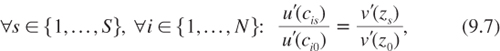
At equilibrium, the marginal rates of substitution between consumption at date 0 and in any specific state at date t are equalized across agents. They are equal to the marginal rate of substitution of an agent whose consumption is equal to the income per capita at date 0 and in any state at date t, but where the original utility function u is replaced by function v. From now on, this function is referred to as “the utility function of the representative agent.” This agent consumes the income per capita in all states and at all dates. An egalitarian economy composed by N identical agents with this utility function v would price all assets in this economy in exactly the same way as in the unequal economy described in the previous section. This section has shown that the existence of a complete set of competitive markets for Arrow–Debreu securities implies the existence of such a representative agent, as initially shown by Wilson (1968). In the next section, the utility function v of the representative agent is characterized.

CHARACTERIZATION OF THE REPRESENTATIVE AGENT

We have seen in the previous section that the utility function v of the representative agent can be derived from the original utility function by solving the following set of equalities: for all z:

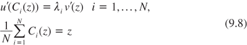
Notice that this set of equations characterizes the solution of the following “cake-sharing” problem:

The competitive allocation of risk maximizes the social welfare in each state of nature, where the social welfare function is the sum of individual utilities weighted by .

The unequal distribution of wealth in the economy is entirely concentrated in the vector of lagrange multipliers (λ₁, …, λ_N). If, for all agents, their endowment has the same market value, the λ_i would all be the same, thereby trivially yielding the solution: v≡ u C_i(z) = z for all z. Suppose alternatively that the market values of the individual endowment are unequal, so that the lagrange multipliers are heterogeneous. Fully differentiating the previous equations with respect to z yields:

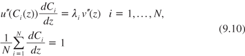
Let T(c) = –u′(c)/u″(c) and T_v (z) = –v′(z)/v′(z) denote the degree of absolute risk tolerance for the utility function of the original agent and of the representative agent respectively. Observe that absolute risk tolerance is just the inverse of absolute risk aversion. Using (9.8), the first equality in (9.10) can be rewritten as:

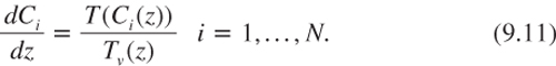
This formula is intuitive. It states that the share of the aggregate risk borne by agent i—which is measured by the sensitiveness of agent i’s consumption to collective income per capita—is proportional to agent i’s degree of absolute risk tolerance. More risk-tolerant agents bear a larger share of the aggregate risk. Using the second equality in (9.10) implies that it must be the case that:

This equation, which was first derived by Wilson (1968), tells us that the degree of risk tolerance of the representative agent is the mean of the absolute risk tolerance of the original agents evaluated at their actual level of consumption. This equation fully characterizes the utility function v of the representative agent in this unequal economy. Once v is obtained, it is possible to determine the socially efficient discount rate by using the standard pricing formula in the canonical model:

where z_t is the random variable which is distributed as (z₁, p₁; …; z_S, p_S). It is obtained, as usual, by considering a marginal investment project in which the income per capita at date 0 is reduced by ε to increase the income per capita in all states at date t by ε exp(r_t). The r_t defined in (9.13) is the one for which, at the margin, this investment project has no effect on the intertemporal social welfare (v(z₀)+e^–δtEv(z_t)). It is assumed that benefits and costs are added and subtracted to aggregate wealth, and are then reallocated in the population according to the cake-sharing rule derived from program (9.9) and described by rule (9.11). In other words, this means that markets for Arrow–Debreu securities remain active after the investment decision is made.

THE IMPACT OF WEALTH INEQUALITY ON THE EFFICIENT DISCOUNT RATE

In order to explore the effect of wealth inequality on the efficient discount rate, let us first examine the special case of an economy in which agents have the same classical power utility function with u′(c) = c_–γ. This implies that T (c) = c/γ, which in turn implies that:

The implication is that the utility function of the representative agent is also a power function, with the same constant relative risk aversion as u. This proves that, under this specification, wealth inequality has absolutely no effect on the shape of the utility function of the representative agent, and therefore on the efficient discount rate. The power utility function is widely used by economists; therefore it can be concluded that the presence of (large) wealth inequalities around the world is not enough, in itself, to justify a departure from the extended Ramsey rule which also relies on a power utility function.

More generally, if the utility function u exhibits linear risk tolerance, the representative agent will have the same utility function u, whatever the degree of wealth inequality in the economy. By contrast, if the utility function u exhibits a convex risk tolerance T, Jensen’s inequality implies that:

The opposite result holds if risk tolerance is concave. A simple result is obtained in the special case of a certain growth rate between dates 0 and t. Suppose that T is convex, so that T_v(z) is larger than T(z) for all z. This means that v is less concave than u in the Arrow–Pratt sense, or that there exists an increasing and convex function ξ such that v(z) = ξ(u (z)) for all z. This implies in turn that if z_t ≥ z₀ i.e., if ξ′(u(z₀)), we obtain:

This means that if the sure growth of the economy is positive, and if risk tolerance is convex, then wealth inequality reduces the efficient discount rate. Assuming that economic growth is uncertain makes the problem considerably more complex, because it requires the degree of prudence of the representative agent to be described in addition to their risk tolerance (Gollier 2001).

EPITAPH FOR LONG-TERM RISK-SHARING ALLOCATIONS

Up to now this chapter has assumed that agents can credibly commit to share risk efficiently over long time horizons. This assumption fits quite well with the reality of the western world over time horizons corresponding to life expectancies, in which people can write legally enforceable insurance and credit contracts. The assumption is far from perfect, however, because of the existence of transaction costs and asymmetric information that result in credit constraints for households. Further, if time horizon t exceeds the lifetime of the current generation, risk-sharing arrangements can only be implicit, which raises a commitment problem. An alternative view is that the agents described earlier are governments that commit their citizens to intergenerational risk-sharing contracts. However, this is quite unrealistic. Even within the European Union, countries have only limited commitments to assist other countries in economic distress, as illustrated by the absence of solidarity within the EU during the financial crisis observed since 2008.

The potential social value of international risk-sharing is enormous, in particular when a long-term perspective is taken. Imagine, for a moment, Marco Polo as a plenipotential ambassador for the western world going to China to sign a treaty of risk-sharing with the eastern world, each party committing to financially compensate the other in case of a persistent divergence in their respective growth rates. Imagine for another moment that today we were able to create a global “Commonwealth” for a progressive mutual assistance scheme where unlucky countries would get positive transfers from the lucky ones over the next two centuries. In both these examples, there exists a large set of mutually beneficial risk-sharing contracts, which are not currently implemented—even at the margin—because of the huge commitment and moral hazard problems that they would generate.

This means that the model presented earlier in this chapter is unrealistic, in particular for the time horizons that correspond to global investment projects and sustainable development generally. It is a useful benchmark, however, since it is the classical model used in the modern theory of finance, which relies heavily on the existence of a representative agent.

THE CASE OF INEFFICIENT RISK SHARING

We hereafter take dynastic or country-specific consumption growth as completely exogenous. An extreme interpretation of this model is that there are no transfers at all between parties in this community, and that each agent consumes at each date its exogenous endowment of the consumption good. Let c_it denote the consumption of agent i at date t. The dynamic stochastic process of (c₁, …, c_N) is not specified at this stage, but it may exhibit temporal and geographical correlations. Intertemporal marginal rates of substitution are not equalized between agents because this allocation is not Pareto efficient. This implies that agents will in general use different discount rates to evaluate any reallocation of consumption through time. It also means that, contrary to the case of efficient risk-sharing examined earlier in this chapter, the law of a single discount rate (for a specific time horizon) is lost. The discount rate to be used to evaluate a collective investment project depends upon how costs and benefits are allocated within the economy.

Let us consider an “egalitarian” investment project that allocates costs and benefits in a non-discriminatory way. More specifically, consider a safe investment project that reduces consumption of all agents by ε at date 0, and that raises consumption of all agents by ε exp(r_tt) at date t. We are looking for the critical internal rate of return for the project that has no effect at the margin on intertemporal social welfare. Intertemporal social welfare is defined, as before, as the discounted sum of the flow of temporal welfare. The welfare at date t is arbitrarily defined as the sum of the individual felicities weighted by Pareto weights (q₁, …, q_N), with Σ_i q_i = 1. Thus, the objective function is defined as:

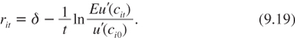
Following the same path as in chapter 2, the critical internal rate of return of the safe project is characterized by the following rule:

Consider the efficient discount rate that should be used by agent i if they alone bear the full costs and benefits of the project:

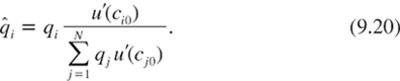
Following Emmerling (2010), let us also define the inequality-neutral Pareto weights such that:

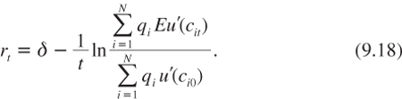
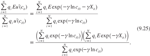
Using equation (9.18), it is then easy to check that the efficient discount rate r_t for an egalitarian cash flow at date t is linked to the individual discount rates (r_1t, …, r_Nt) in the following way:

The efficient discount factor is a weighted mean of the individual discount factors. This is reminiscent of equation (6.4) that describes the term structure of efficient discount rates when there is a single representative agent with utility function u, but in which there is some uncertainty about the true stochastic process for the growth of per capita consumption. Equation (9.21) describes the efficient discount rate in an economy with a representative agent who faces a stochastic process c_it with probability i = 1, …, N. In this model, there is therefore a formal equivalence between the fact that different agents may face different destinies, and the fact that all agents face the same uncertain destiny. This equivalence is an illustration of John Rawls’ concept of the veil of ignorance. It follows that the analysis in this section can be limited by referring to the results presented in chapter 6. For example, for distant time horizons, the efficient discount rate tends to the smallest individual long-term discount rate. The equivalence with the model of parametric uncertainty is perfect only when there is no inequality of consumption at date 0; otherwise the Pareto weights need to be biased.

To illustrate, consider a specification similar to that which was examined in chapter 6:

Under constant relative risk aversion γ, it implies that:

Combined with equation (9.21), this implies that the efficient discount rate r_t is decreasing and tends to the smallest r_i when t tends to infinity. Moreover, r_t satisfies the following property:

The short-term discount rate is the weighted mean of the individual discount rates. The intuition is the same as in the framework of parametric uncertainty. For the very distant future, what really matters when evaluating a project is whether it can improve the welfare of the poorest agent. The true shape of the term structure depends upon the distorted Pareto weights which depends upon our ethical values (q₁, …, q_N), the initial degree of inequality (c₁₀, …, c_N0), and its correlation with the distribution of economic growth.

ECONOMIC CONVERGENCE AND THE DISCOUNT RATE

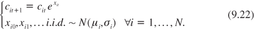
In order to have a more precise description of the term structure, it is necessary to specify the degree of convergence of economic development. Let us first consider an economy without any convergence, in which the current level of development of a country is uninformative about its future economic growth. More precisely, suppose that log c_i0 is independent of the distribution of the growth rate x_it. Let X_it be the cumulative growth of log consumption between 0 and t. Under constant relative risk aversion γ, this implies that:

The second equality is a direct consequence of the no-convergence hypothesis. This implies in turn that:

This means that the term structure of discount rates is independent of the initial distribution of wealth in this framework. Only the unequal expectation about future growth matters.

Let us now consider the case of economic convergence. An economy is characterized by its initial allocation of consumption c₀~(c₁₀,q₀;…;c_N0’,q_N) and by its individual expectations X_t~(X_1t,q₁;…;X_Nt,q_t). Following Gollier (2010), it can be said that economic convergence increases in this economy if the pair of random variables (ln c₀, X_t) becomes less concordant, as defined in chapter 8. Remember that this means that the new distribution of (ln c₀, X_t) is obtained from the initial one by a sequence of marginal-preserving reductions in concordance. In other words, for initially poor agents, growth prospects are FSD-improved, whereas they are FSD-deteriorated for the initially wealthy agents. Those transfers in probability are made in such a way that the unconditional distribution of growth is unchanged.

Lemma 2 in chapter 8 is useful for evaluating the impact of economic convergence on the efficient discount rate. Observe that the numerator in the right-hand side of equation (9.18) can be expressed as:

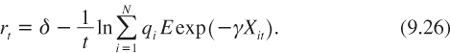
Lemma 2 in chapter 8 tells us that a reduction of concordance of ln c₀ and X_t, that is an increase in economic convergence, reduces this numerator if and only if h(x₁,x₂) = u′(exp(x₁ + x₂)) is supermodular. This is true if and only if relative prudence is uniformly larger than unity. Therefore, it can be concluded that economic convergence raises the efficient discount rate if relative prudence is larger than unity. This is the case, for example, with constant relative risk aversion, for which equation (9.26) underestimates the true discount rate for all time horizons. Symmetrically, economic divergence tends to reduce the discount rate. This is reminiscent of the idea that saving and investing are a substitute to the reduction of future risks.

To illustrate, consider a global economy with two equally populated countries. Country i = 1 has a GDP per capita at date 0 that is normalized to one. Country i = 2 has a GDP per capita at date 0 that is fifty times larger. Our ethical values impose q₁ = q₂ = 1/2. Suppose that, in economy A, the two countries converge, with country 1 enjoying a constant growth rate of 3%, whereas the growth rate of the wealthier country 2 is only 1%. These growth rates imply that the two countries will have the same per capita consumption level in just a bit less than two hundred years. Consider alternatively an economy B with the same initial distribution of consumption levels, (c₁₀, c₂₀) = (1, 50), but the same uncertain growth rate for the two countries, which will be either 1% or 3% with equal probabilities. Clearly, economy A exhibits more economic convergence than economy B, as defined. In figure 9.1, we have drawn the term structure of efficient discount rates in these two economies. As expected, the two curves are decreasing, and the discount rates are larger when there is convergence.

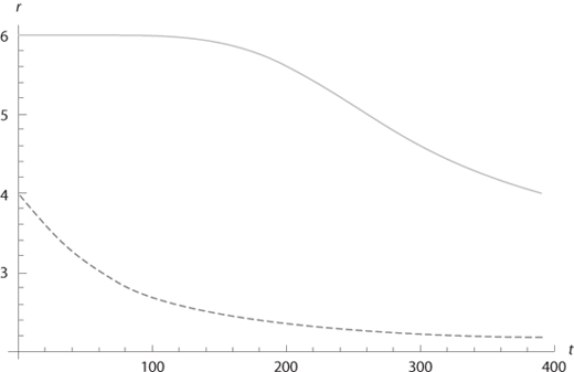
Figure 9.1. Term structure in a two-country model with (c₁₀, c₂₀) = (1, 50) and (x_1t, x_2t) = (3%, 1%). It is assumed that γ = 2 and δ = 0%. The dashed curve corresponds to the case where the two countries face an uncertain constant growth rate of either 1% or 3% with equal probabilities.

A SIMPLE CALIBRATION EXERCISE

What is known about economic convergence? The classical economic theory of economic growth provides an argument for it, since decreasing marginal productivity of capital implies that wealthier countries should grow at a smaller rate. Furthermore, poorer countries can replicate successful production methods, technologies, and institutions which were implemented earlier by more developed countries. However, in spite of the existence of some successful newly developed countries such as India, Singapore, South Korea, China, or Brazil, many poor countries seem to be permanently underdeveloped, whereas some others are becoming ever poorer (for example, Haïti and Zimbabwe). According to Clark (2007), the industrial revolution has reduced inequalities within societies, but it has increased them between societies. This process has been labeled “the Great Divergence” (Pomeranz 2000).

Accepting that history is full of periods of global divergence, in contrast the last forty years have been characterized by a global convergence between countries. In the following calibration exercise, the focus is on estimating the level of convergence during the period 1969 to 2009. The calibration examined in Gollier (2010) is based on the ERS International Macroeconomic data set that gives us estimation of the GDP per capita for 190 countries during this period. A set of thirteen regions that are relatively homogenous in size and in socioeconomic structure were defined because of the extremely large heterogeneity of the 190 country sizes. This data set is summarized in table 9.1 and figure 9.2.

Let us first assume that there is no economic convergence. Under the assumption of constant absolute risk aversion, we know that the initial inequalities do not matter for the determination of the discount rate. Equation (9.26) can therefore be used, which is rewritten as:

TABLE 9.1.
Global economic convergence during the period 1969–2009

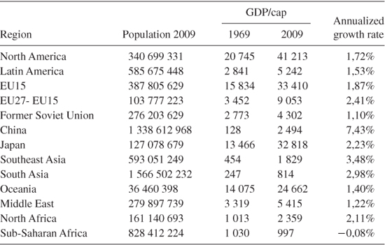
Source: ERS International Macroeconomic data set

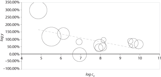
Figure 9.2. Global economic convergence over the period 1969–2009. c₀ is the GDP/cap in 1969 (expressed in USD of 2005), and X = ln y is the total growth rate over the period. The surface of the circle is proportional to the population size in 2009. Source: ERS International Macroeconomic data set.

The regional data set previouslydescribed yields μ = E ln X_t = 0.9047 and σ² = Var ln X_t = 0.5128. Assuming that ln X_t is normally distributed, γ = 2 and δ = 0, lemma 1 implies that:

It is notable that this calibration, based on a comparison of the growth rates of thirteen regions during the same period, generates a much smaller discount rate than the 3.6% obtained in chapter 3 using the growth rate of the U.S. economy throughout the twentieth century. This is because the annualized standard deviation of growth rates is much larger in the cross-section data (11.3%) than in the time-series data of the U.S. economy (3.6%). The precautionary effect is therefore much larger.

Let us now recognize that economic growth rates across regions are not independent. The degree of economic convergence is estimated through the following simple regression:

The t-statistic of the slope coefficient β equals –2.41, so that it is significantly different from 0. The R² of the regression is 0.35. Therefore, economies are converging. Notice that this is mostly due to the extraordinary growth rates observed in China and India in the last two decades.

These numbers can be plugged into equation (9.18), weighting countries by their population in 2009. It follows that:

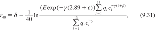
where c_i is the GDP per capita of region i in 2009, and β = –0.26. Using lemma 1 with the fact that the variance of the residuals in (9.30) is Var ε = 0.31 gives r₄₀ = 4.06%. The effect of economic convergence, which is positive as expected, is surprisingly large.

SUMMARY OF MAIN RESULTS

1.  The (extended) Ramsey rule is based on the assumption of the existence of a representative agent. This is a meaningful assumption if the heterogeneity of preferences and of incomes is limited. Alternatively, we have shown that there exists a representative agent if risks and credit are efficiently allocated in the economy.

2.  Under the assumption of an efficient risk and credit allocation, inequilities are irrelevant for the discount rate if relative risk aversion is constant. In the absence of risk on growth, the impact of inequalities on the discount rate depends upon whether absolute prudence is concave or convex in consumption.

3.  Because of agency problem, global long-term risks are not efficiently shared. Behind the veil of ignorance, inequalities in the growth of individual consumption play a role equivalent to parametric uncertainty, as examined in chapter 6.

4.  Behind the veil of ignorance, economic convergence reduces the long-term risk on consumption, thereby raising the long discount rate under prudence.

REFERENCES

Clark, G. (2007), A Farewell to Alms: A Brief History of the World, Princeton: Princeton University Press.

Emmerling, J. (2010), Discounting and intergenerational equity, mimeo, Toulouse School of Economics.

Gollier, C. (2001), Wealth inequality and asset pricing, Review of Economic Studies, 68, 181–203.

Gollier, C. (2010), Discounting, inequalities and economic convergence, mimeo, Toulouse School of Economics.

Gollier, C., and R. J. Zeckhauser (2005), Aggregation of heterogeneous time preferences, Journal of Political Economy, 113, 878–898.

Pomeranz, K. (2000), The Great Divergence: China, Europe, and the Making of the Modern World Economy, Princeton: Princeton University Press.

Wilson, R. (1968), The theory of syndicates, Econometrica, 36, 113–132.

¹Gollier and Zeckhauser (2005) examine the effect of heterogeneous rates of impatience.