11

Alternative Decision Criteria

The discounted expected utility (DEU) model that is used in this book is not without its critics. Since Allais (1953), many researchers have found contexts in which human behavior is incompatible with the DEU model. It is clear that the model is violated by many people, in many contexts. Some of these violations are informative about the true nature of individuals’ actual preferences, whereas others are generated by errors, biased beliefs, lack of information, or a lack of time and effort spent on finding the optimal strategy. These violations imply that the DEU model is not very good for explaining, or predicting, actual behaviors under uncertainty. However, the aim of this book is not positive, it is normative. The interest is not directly in what people actually do, but instead to determine what they should do.

Many experiments stress the weakness of the independence axiom (IA), which is the cornerstone of the von Neumann–Morgenstern expected utility theory. The IA can be illustrated as follows. Suppose that, for tonight, you are offered tickets for the theater or a meal at a restaurant. Which do you prefer? Suppose that you prefer to go to the restaurant. Now, you are told that the theater and the restaurant are downtown. The only way to get there is to take the subway because you live in the suburbs. The problem is that there is a 10% probability that the subway will be on strike. Therefore, the actual decision choice that you face is not whether you prefer to go to the restaurant with certainty, or to go to the theater with certainty. The actual choice is whether you prefer lottery R to lottery T, where lottery R is a good dinner at the restaurant with probability 0.9, or staying at home with probability 0.1, and lottery T is a nice evening at the theater with probability 0.9, or staying at home with probability 0.1. The IA claims that it is natural to assume that the fact that there is now a 0.1 probability of staying at home, whatever choice you make, should not change your initial preference. If you prefer the restaurant to the theater in the certainty case, you should also prefer lottery R to lottery T. This is intuitive, and it is desirable that our collective preferences satisfy this axiom. Although many people violate this axiom, as cleverly shown by Allais (1953), we want to rely on this axiom to drive public decisions.

Several interesting decision criteria, which provide an alternative to the expected utility model, have blossomed over the last three decades. Most of them violate the independence axiom, and will not be examined here. The aim in this chapter is to describe a sample of the alternative decision criteria that have features which are normatively attractive.

RECURSIVE EXPECTED UTILITY

The concavity of the utility function plays two roles in the DEU model. The index –/u′ measures the aversion to consumption inequalities across time and across states of nature. The first feature yields the crucial wealth effect in the Ramsey rule, whereas the second is linked to risk aversion and to prudence. It is possible to question the logic for decreasing marginal utility of consumption generating both an aversion to risk within each period as well as an aversion to non-random fluctuations of consumption between periods. If the marginal welfare gain from k more units of consumption is less than the marginal loss owing to k units of reduction in consumption, agents will reject the opportunity to gamble on a fifty-fifty chance to gain or lose k units of consumption. For the same reason, if their current consumption plan is constant, patient consumers will reject the opportunity to exchange k units of consumption today against k units of consumption tomorrow. Kreps and Porteus (1978), Selden (1979), and Epstein and Zin (1991) claimed that there is no logical reason to impose the use of the same utility function for both of these psychological processes. They proposed an alternative model which disentangles attitudes toward consumption smoothing over time and across states. Following Gollier (2002) and Traeger (2009), this section summarizes the application of this model to the problem of evaluating a safe investment project.

The analysis is limited to a model with two dates. As before, let c₀ and c₁ denote consumption per capita respectively in the present and in the future. Welfare at date 0 is evaluated “recursively” by backward induction, in two steps. The certainty equivalent m of future consumption, c₁, is evaluated first by using an increasing and concave von-Neumann–Morgenstern utility function v:

A time-aggregating utility function u is then used to evaluate intertemporal welfare W:

The utility function v characterizes attitudes toward risk, whereas function u characterizes attitudes toward time. The reader can easily check that the standard DEU model is recovered if the functions u and v are identical. If v is linear, it follows that m = Ec₁ and the agent is risk-neutral. This is compatible with a positive wealth effect in the Ramsey rule if u is concave and Ec₁ > c₀. In other words, one can be risk-neutral and have a preference for a reduction in consumption fluctuations over time. Symmetrically, one can be risk-averse and, at the same time, neutral toward consumption fluctuations over time. This would be the case if v is concave and u is linear. To sum up, –/v′ measures risk aversion, whereas /u′ measures aversion to intertemporal inequality of consumption.

Consider a safe investment project that generates, at date 1, exp(r) monetary units per monetary unit invested at date 0. A marginal investment in this project has no effect on intertemporal welfare W if:

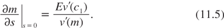
where m = m(0) and m(s) is defined as follows:

It yields:

All this implies that the efficient discount rate equals:

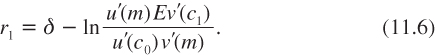
When u ≡ v, the standard pricing formula used in this book is recovered. Let us first examine the wealth effect as in chapter 2. Suppose that c₁ is safe, so that m = c₁. In that case, equation (11.6) simplifies to (3.16) with t = 1.

The analysis of the precautionary effect is more complex than in chapter 3. In the following, the condition under which adding a zero-mean risk to c₁ reduces the efficient discount rate is determined. Using (11.6), this is the case if and only if:

or equivalently, if:

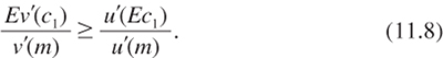
Observe first that the right-hand side of this inequality is less than unity, because m is larger than Ec₁ under risk aversion. This upper bound is attained when the representative agent has a neutral attitude toward consumption inequalities over time. Thus, inequality (11.8) will surely hold if its left-hand side is greater than unity, that is, if Ev′(c₁) is greater than v′(m) Let x = v(c₁) and g(x) = v′(v^–1(x)). With this notation, this condition can be rewritten as:

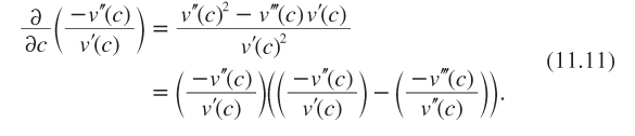
By Jensen’s inequality, this is the case if and only if g is convex. Because g(v(c)) = v′(c) it is obtained that:

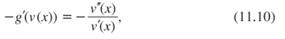
This immediately implies that g is convex if and only if v exhibits decreasing absolute risk aversion (DARA).

It can be concluded that the precautionary effect on the discount rate is negative, as in the standard DEU model, if v exhibits DARA. This condition is necessary and sufficient if u is linear. It is notable that DARA is a condition that is stronger than prudence since

The implication is that DARA holds if and only if prudence is greater than risk aversion. It should not be a surprise that a more general model than the DEU model generates more demanding conditions for a specific comparative static property (precautionary saving).

This model can be calibrated using power utility functions and a lognormal distribution for c₁:

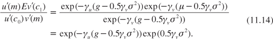
Observe that function v exhibits DARA, therefore a negative precautionary effect must be expected. Using lemma 1, it follows that:

with g = μ +0.5σ². This in turn implies that:

This implies that the socially efficient discount rate equals:

In the DEU case, with γ_u = γ_v, this formula is equivalent to equation (3.23). This shows that the model does not radically modify our understanding of the determinants of the efficient discount rate. In the short run, the driving force of the discount rate is the wealth effect, which is the same as in the DEU case. Because σ² is small, changing the precautionary effect from 0.5γ_u(γ_u + 1)σ² does not affect r₁ very significantly. An appraisal of the effect of γ_v ≠ γ_u for the long-term discount rate remains to be made.

MAXMIN AMBIGUITY AVERSION

In chapter 6, models in which the true probability distribution of future consumption, c₁, is uncertain were examined. The DEU model was used to evaluate safe projects under this two-stage risk context, with stage 1 being the random selection of the true distribution, and stage 2 being the random draw of the realization of c₁ from this distribution. Since Ellsberg (1961), it has been known that many people do not evaluate such a two-stage risk in a way that is compatible with the DEU model.

Let us consider a simplified version of the Ellsberg game. Consider an urn that contains 100 balls, some are black, and the others are white. The two games that will be considered have the same basic structure. The player must pay an entry fee to play the game. The player bets on one of the two colors. The experimenter randomly extracts a ball from the urn, and pays 1,000 euros to the player if the color of the ball corresponds to the one on which they bet. In the first game, which is referred to as the “risky game,” there are exactly 50 black balls and 50 white balls. Betting on either of the two colors yields the same lottery to win 1,000 euros with probability ½, therefore most people are indifferent as to which color they bet on. The entry fee that individuals are ready to pay is less than the expected gain of 500 euros because of risk aversion.

Consider alternatively the “ambiguous game,” in which the player gets no information about the proportion of black and white balls in the urn. The closed ambiguous urn is brought in front of the player before the player selects the color to bet on. What is usually observed in this second experiment is that most people are still indifferent between betting on white or on black, but that they are ready to pay much less to play this ambiguous game than the risky game. This cannot be explained under the DEU model. Indeed, if the player is indifferent between white or black, this must mean that they believe that their chance to win by betting white is the same as by betting black. This implies that their expected probability to win is ½ because the probabilities must sum up to unity, independently to the color on which the player bets. The player therefore faces a lottery to win 1,000 euros with probability ½, which is the same lottery as in the risky game. The player should thus be ready to pay the same entry fee in the two games. The fact that most people are ready to pay much less for the ambiguous game than for the risky game tells us that people are ambiguity-averse, a psychological trait that cannot be explained by the DEU model. Ambiguity aversion just means that people prefer a lottery to win a widget with a sure probability p than another lottery to win the same widget with an ambiguous probability with mean p.

The first attempt to produce a decision criterion that produces ambiguity aversion was made by Gilboa and Schmeidler (1989). Suppose that people form an expectation about the set of plausible distributions of the random variable x that they face. A form of ambiguity aversion is obtained if we state that agents evaluate their welfare, ex ante, once their choice has been made, by the minimum expected utility over a set of plausible probability distributions. This “maxmin” criterion would explain the behavior observed in the Ellsberg game. Indeed, suppose that people form their beliefs such that the probability of a white draw is either 0.25 or 0.75. If they bet on white, people will compute their welfare by assuming that there are only 25 white balls. If they bet on black, they will do so by assuming that there are only 25 black balls. Thus, under the maxmin criterion, their welfare will be measured by the expected utility of 1,000 euros with the minimum plausible probability, which is 0.25, whether they bet on white or on black. The certainty equivalent of that lottery is indeed much smaller than in the risky game in which the probability to win is 0.5.

Let us apply this idea to the discounting problem. To retain the notation used earlier, suppose that the distribution of c₁ depends upon an unknown parameter θ that can take n possible values θ = 1, …, n. Let θ = 1 denote the value of the parameter that yields the smallest expected utility at date 1. The efficient discount rate would then satisfy the standard pricing formula (3.16), but in which the distribution of c₁ would be c₁ | θ = 1 rather than the unconditional distribution of c₁ as assumed in chapter 6. What would the consequences be for the short-term efficient discount rate r₁? Suppose that the uncertainty is about the mean growth rate. In that case, ambiguity aversion would replace the mean growth rate by the minimum growth rate in the Ramsey rule. Suppose alternatively that the uncertainty is about the volatility of the growth rate. In that case, ambiguity aversion would replace the mean volatility by the maximum volatility in the Ramsey rule. In the two cases, the problem becomes equivalent to computing the discount rate that would be efficient conditional on each realization of θ, and then selecting the smallest of these rates as the efficient discount rate r₁. Interestingly enough, in the case of a random walk, the short-term discount rate that is efficient under the maxmin theory is the discount rate that is efficient for the distant future in the DEU model examined in chapter 6.

SMOOTH AMBIGUITY AVERSION

There are difficulties using the maxmin model in order to provide normative recommendations. This is because it does not explain how to determine the set of plausible distributions that is part of the preferences of the representative agent. This is problematic because this model is very sensitive to the characteristics of the worst probability distribution, which could be arbitrarily catastrophist. Klibanoff, Marinacci, and Mukerji (KMM, 2005, 2009) have recently proposed a model that is easier to implement, and is less sensitive to the extreme plausible distribution. They define ambiguity aversion as the aversion to any mean-preserving spread in the space of probabilities. Remember that risk aversion is an aversion to any mean-preserving spread in the space of payoffs. For example, risk aversion means that one prefers to get 500 in two equally probable states, than to receive 1,000 in state 1, and 0 in state 2. Taking this risky lottery as a benchmark, ambiguity aversion means that one prefers a lottery in which the true probability of state 1 is 0.5 with certainty rather than a lottery where the probability of state 1 is either 0.25 or 0.75 with equal probabilities. The maxmin model examined earlier is an extreme version of aversion to mean-preserving spreads in the space of probability distributions.

KMM have proposed the following decision criterion under ambiguity. For each possible value of θ, the conditional expected utility E[u(c₁)|θ] is computed. In the standard DEU criterion used in chapter 6, we just take the mean of the conditional expected utilities under the subjective distribution (q₁, …, q_n) of θ. Rather than doing this, we take its certainty equivalent by using an increasing and concave function φ:

Because φ is concave, M is smaller than the unconditional expected utility, which means that this welfare function exhibits ambiguity aversion. It is helpful to examine two special cases. First, if function φ is the identity function, then this welfare function is the same as in the standard DEU case, in which agents are neutral to mean-preserving spreads in probabilities. The expected utility criterion is linear in probabilities. In fact, function () is an index of absolute ambiguity aversion. The other special case is obtained by assuming that , where the index of absolute ambiguity aversion A_ϕ tends to infinity. It was demonstrated in chapter 6 that Eϕ(u) tends to the minimum of u in that case, so that we get the maxmin criterion as another special case.

As usual, let us consider a safe investment project that yields exp(r) monetary units at date 1 per monetary unit invested at date 0. At the margin, this project has no effect on intertemporal welfare, W, if:

This yields the following efficient discount rate:

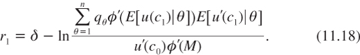
Gierlinger and Gollier (2011) illustrate two effects of ambiguity aversion in this model: an ambiguity prudence effect and a pessimism effect. The ambiguity prudence effect is easiest to explain if it is assumed that the representative agent is risk-neutral, that is, if u is the identity function. This switches off both the wealth effect and the precautionary effect of the standard DEU model. In that case, equation (11.18) simplifies to

where is the conditional expected consumption at date 1. Therefore, the ambiguous distribution of economic growth reduces the efficient discount rate if:

Exactly the same technical condition was encountered in the section on recursive expected utility (see condition (11.8)), where it was shown that it requires that the φ function exhibits decreasing absolute aversion: ()′ ≤ 0. We refer to this condition as “decreasing absolute ambiguity aversion” (DAAA). Duplicating this proof, define function g(x) = φ′(φ^-1(x)) and . Condition (11.20) can then be rewritten as Eg(x) ≥ g(Ex), where x is distributed as (x₁,a₁;…;x_nq_n). The proof is concluded by observing that this is the case if g is convex, which is equivalent to DAAA. This is more demanding than requiring the prudence of φ (φ′″ ≥ 0). This ambiguity prudence condition guarantees that, under risk-neutrality, the existence of some ambiguity on the distribution of future consumption reduces the discount rate.

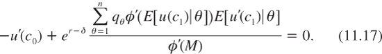
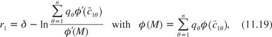
The pessimism effect is similar to the one that is obtained under the maxmin criterion. It is easiest to illustrate by switching off the ambiguity prudence effect, that is, by assuming that absolute ambiguity aversion is constant. If it is assumed that φ(u) = –A _φexp(-A _φu), it follows that φ’(M) equals Σ_θq_θφ′(Eu_θ). This implies that equation (11.18) can be rewritten as:

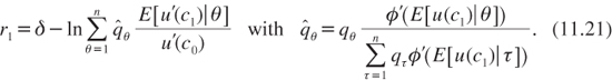
If this discount rate is compared to the one that was obtained under the standard DEU criterion, which is equation (6.2) with t = 1, it can be observed that the only difference is that the beliefs described by (q₁, …, q_n) have been distorted, becoming (₁, …, _n) defined in (11.21). Because φ′ is decreasing, these distorted beliefs put more probability weight on the θ that yields a smaller conditional expected utility. This is a clear expression of pessimism, whose extreme version was illustrated by the maxmin model. If it is supposed, for example, that there is uncertainty about the expected growth rate, the probabilities will be distorted in favor of the θ with the smallest expected growth rate, for which the expected marginal utility is larger. This will tend to reduce the discount rate r₁.

To sum up, ambiguity aversion tends to reduce the discount rate. One can illustrate this intuitive idea by considering the following specification suggested in Gierlinger and Gollier (2011). Suppose as in chapter 6 that ln c_t θ is normally distributed with mean ln c₀ + μ θt and variance σ²t. Suppose that the mean of the change μ_q in the log of consumption is itself normally distributed with mean μ₀ and variance. Consider the case of a power utility function with constant relative risk aversion g. This model is exactly the benchmark case that was considered in chapter 6. The only new dimension is ambiguity aversion. Suppose that θ exhibits constant relative ambiguity aversion . Using lemma 1 twice, Gollier and Gierlinger (2011) obtained the following formula:

where is the growth rate of expected consumption. This equation should be compared to equation (6.13), which is a special case of (11.22) with h = 0. This observation allows us to conclude that ambiguity aversion yields a new determinant to the discount rate, which, under the specification considered here, is negative and linear with the time horizon. This is because, with an uncertain trend in economic growth, the degree of ambiguity is magnified by the time horizon in this framework.

It is noteworthy that Gierlinger and Gollier (2011) show that the introduction of ambiguity aversion does not always reduce the discount rate, even under decreasing absolute ambiguity aversion.

INTERGENERATIONAL HABIT FORMATION

Although the current generation consumes considerably more goods and services than their parents, they are not really happier. This is a paradox. The indices of happiness do not parallel those of GDP per capita (see for example Layard 2005). One possible explanation is that people evaluate their well-being in relative rather than in absolute terms. In particular, their felicity at date t is not a function of their consumption at date t alone. In the literature on external habit formation, it is assumed that the agent’s felicity at date t is a function of c_t and of a weighted average of past consumption(c_t-1,c_t-2’…). This breaks down the time-additivity property of the DEU model. Constantinides (1990) has argued for a positive effect of past consumption on today’s marginal utility of consumption, which is a simple definition of a consumption habit. A large consumption level in the past raises the marginal utility of current consumption, thereby creating some form of addiction to consumption.

A simple specification is the multiplicative habit in which the felicity at date t is measured by , for some positive constant α ≤ 1. A special case is α = 1, in which case the felicity is a function of the growth rate of consumption rather than of the level of consumption. For example, if the growth rate of consumption is a positive constant, the felicity will remain constant over time in this model. Under these preferences, at any time, a temporary increase in consumption above its historical trend is beneficial in the short run, but generates a negative externality for future welfare because of the consumption habit that this transitory increase generates. When a is less than unity, this negative externality is reduced. Therefore, a is a measure of the degree of habit formation.

To keep the model simple, let us assume that u(x) = x^1-γ/(1-γ) with γ >1. Suppose also that the growth rate of consumption is a positive constant g. Observe now that

with γ’ = α + (1-α)γ. This shows that the existence of a multiplicative internal consumption habit transforms the intertemporal welfare function in a very simple way. First, it multiplies the felicity by a common positive constant e^αg(1-γ). Second, it modifies the degree of relative risk aversion from γ to γ′, which is the mean of γ and 1 weighted respectively by (1–α) and α. Since it is usually assumed that γ is larger than unity, this model of habit formation just reduces the degree of concavity of the felicity function. The Ramsey rule (2.12) therefore still holds, but with γ being replaced by the smaller γ’

Owing to a consumption habit downsizing the wealth effect, it yields a smaller discount rate. The intuition is that investing for the future is a good way to impose self-control on today’s level of consumption, thereby limiting the formation of consumption habits that have adverse effects on future welfare. Gollier, Johansson-Stenman, and Sterner (2010) extend this result to the case of uncertainty.

The internal habit formation model briefly described earlier has some interesting features with which to explain observed human behaviors. For example, it can contribute to solving the equity premium puzzle (Constantinides 1990). However, it is still an open question whether or not this model should be used for normative analysis of public policies spanning several generations. It is clear that parents transfer consumption habits to their children, so that habit formation is not strictly speaking an intra-individual feature. But is it enough to justify more sacrifices from the current generation?

Many other models alternative to DEU could have been considered for inclusion in this chapter, but to be concise, decisions had to be made. Other models that could have been discussed include, for example, the cumulative prospect theory introduced by Tversky and Kahneman (1992). This model shares with the habit formation model the idea that future consumption will be evaluated in relation to some reference point that may be related to past consumption. But prospect theory also has other features, such as the assumption that agents are risk-lovers over a range of losses below the reference point. It is also assumed that they distort the distribution function by using some specific nonlinear function that plays a role symmetric to the utility function that transforms payoffs into utility in a nonlinear way. This transformation raises the subjective probability of extreme events, which has the effect of raising the precautionary term in the extended Ramsey rule, thereby reducing the discount rate. It is still too early to determine which of these innovations will survive the rigors of the scientific validation process over the longer term.

SUMMARY OF MAIN RESULTS

1.  A standard critique made to the discounted expected utility model is that the concavity of the utility function expresses at the same time the aversion to inequalities and the aversion to risk. Moreover, it does not take account the possibility of an aversion to ambiguity on probabilities, or the formation of consumption habits.

2.  Recursive preferences à la Kreps-Porteus-Epstein-Zin allows for disentangling the aversion to intertemporal inequalities and the aversion to risk. The extended Ramsey rule is easily adapted to this generalization of the DEU model.

3.  Ambiguity about the distribution of future economic growth was introduced in chapter 6 with uncertainty about the parameter of the stochastic process. Ambiguity aversion has two effects on the term structure of discount rate. First, it implies pessimism about the trend or about the volatility, thereby reducing the level of the term structure. Second, because ambiguity is increasing with maturity, it makes the term structure more downward sloping.

4.  Habit formation is introduced in the DEU model by making instantaneous felicity a function of past consumption. It weakens the wealth effect, thereby reducing the discount rate.

REFERENCES

Allais, M. (1953), Le comportement de l’homme rationnel devant le risque, Critique des postulats et axiomes de l’école américaine, Econometrica, 21, 503–546.

Constantinides, G. (1990), Habit formation: a resolution of the equity premium puzzle, Journal of Political Economy, 98, 519−543.

Ellsberg, D. (1961), Risk, ambiguity, and the Savage axioms, Quarterly Journal of Economics, 75, 643–669.

Epstein, L. G., and S. Zin (1991), Substitution, risk aversion and the temporal behavior of consumption and asset returns: An empirical framework, Journal of Political Economy, 99, 263–286.

Gierlinger, J., and C. Gollier (2011), Socially efficient discounting under ambiguity aversion, mimeo, Toulouse School of Economics.

Gilboa, I., and D. Schmeidler (1989), Maxmin expected utility with a non-unique prior, Journal of Mathematical Economics, 18, 141–153.

Gollier, C. (2002), Discounting an uncertain future, Journal of Public Economics, 85, 149–166.

Gollier, C., O. Johansson-Stenman, and Th. Sterner (2010), Ramsey discounting when relative consumption matters, mimeo, Toulouse School of Economics.

Klibanoff, P., M. Marinacci, and S. Mukerji (2005), A smooth model of decision making under ambiguity, Econometrica, 73(6), 1849–1892.

Klibanoff, P., M. Marinacci, and S. Mukerji (2009), Recursive smooth ambiguity preferences, Journal of Economic Theory, 144, 930–976.

Kreps, D. M., and E. L. Porteus (1978), Temporal resolution of uncertainty and dynamic choice theory, Econometrica, 46, 185–200.

Layard, Richard (2005), Happiness: Lessons from a New Science, London and New York: Penguin Press.

Selden, L. (1979), An OCE analysis of the effect of uncertainty on saving under risk independence, Review of Economic Studies, 46, 73–82.

Traeger, C. P. (2009), Recent developments in the intertemporal modeling of uncertainty, Annual Review of Resource Economics, 1, 261–286.

Tversky, A., and D. Kahneman (1992), Advances in prospect theory—Cumulative representation of uncertainty, Journal of Risk and Uncertainty, 5, 297–323.