
Computer assistance in electronics
Drawing a circuit diagram, analysing the action, and subsequently planning and drawing the silk-screen outlines and the copper track plan for a printed circuit board are activities that are rightly regarded as monotonous and liable to error when they are done by the traditional methods. For a considerable time it has been possible for the larger manufacturer to use computers, mainframe or mini, to aid these actions, but at a cost that would be unacceptable for the small-scale designer or the educational user. The standardization of the PC type of machine and the remarkable amount of computing power that modern examples (using the Pentium or equivalent chips) can achieve now bring computer-aided drawing and PCB planning methods within the reach of virtually any user.
The availability of low-cost computers has made it possible to carry out many tasks in electronics with very much less effort than was once required. At the time of writing, a good PC can be bought for as little as £300, and close scrutiny of the computing magazines will show that some names you might think of as supplying ‘basement bargain’ computers are, in fact, suppliers of rather overpriced goods. There is not much relationship between price and reliability, and since all PC machines are basically of the same design (and often share the same PCBs) the facilities on the less costly machines are not necessarily less than on the high-priced ones. As in so many other aspects of life, it is often better to avoid famous brand names unless you like paying for a nameplate, and the content of the boxes is more important than their appearance or their nameplates.
In this chapter, the most important contributions of the PC to electronics are described. These comprise Internet access to information and programs, the drawing of circuit diagrams, the analysis of linear circuits (passive or active), the analysis of digital circuits, and the drafting of printed circuit layouts. All are particularly tedious to carry out by traditional methods, and the use of the computer is an immense saving of time, effort and money, particularly to small firms specializing in one-off equipment. The amateur can also gain considerably from these applications because they provide him/her with methods that were once available only to the largest scale of professional users.
The computer
Any computer that is described as being PC compatible can be used for the type of work described here, but the faster modern PC machines are better suited for all tasks, provided suitable software is available. This excludes machines such as the Acorn Archimedes, Atari ST, Apple Macintosh and Commodore Amiga – the use of the letter A is coincidental but a useful way of remembering that these are the incompatible machines, each of which is made by one manufacturer only.
In general, for the type of software you will use you will need a computer whose typical specification is summed up as follows:
Celeron, Pentium or equivalent processor working at 300 MHz or faster
3 ![]() in floppy drive and fast CD-ROM drive (24× or more)
in floppy drive and fast CD-ROM drive (24× or more)
Fast 56K modem and Internet connection
You may feel that the capabilities of the machines currently on offer are much more than you need, but it is by now almost impossible, other than buying second-hand, to obtain computers of lower standard. There is nothing wrong in buying an older machine, but you should be prepared to replace the hard drive when it fails, and this requires some experience in the repair and software formatting of a computer.
One of the considerable advantages of the PC machines is that the scale of production allows important add-ons like hard disk drives to be available at very low prices as compared with other machines. It is almost impossible to have too much hard disk space (or too much RAM), and the depth of your pocket should be the only limitation.
Internet access
The requirements of a computer for Internet use hinge as much on the modem as on the computer itself. The modem is the hardware item (which uses built-in software) that converts computer signals into tones and vice versa, so that signals can be exchanged using telephone lines that were intended for nothing more than speech. A fairly old computer can be used successfully for browsing the Internet provided that the modem and the browser software will run on that computer. For older machines this rules out the use of the most recent software, such as Microsoft Internet Explorer-5, and since the Internet in its present form has not been around for as long as the PC machine, there is not much software around that can be used on old machines. Older machines cannot make full use of modern fast modems (56K type), so that Internet contact will inevitably be slower. If you have a connection that is virtually free, this is not a worry, but if you are shelling out several pence per minute in telephone charges it can be significant.
• To use the Internet, then, requires software that runs under Windows, and the more modern versions of Windows (95 – version 2 onwards) will provide browser and email software integrated into Windows.
Another point to note is that additional software or information that is needed to make connection is usually supplied by the Information Provider (IP) on CD-ROM, so your computer needs a CD drive to read the software. Some providers will offer the alternative of floppy disks. Many IPs offer free access, so that the only cost is that of telephone time. Others now offer free access (including telephone time) at a fixed rate, typically with a joining fee and a small annual charge.
The hardware that must have priority for any computer used for Internet access is a fast modem. At the time of writing the fastest modems available are the 56K type, but some older computers cannot cope with this modem speed, and even some modern machines can encounter problems, particularly if the operating system is Windows 2000. A machine of the standard described above should be able to cope with a fast modem with few problems.
At the time of writing, the only other options for connections were:
A link through a TV cable operator
An old computer that is fitted with a hard drive, and running Windows (Version 95 onwards) can probably be used for Internet access. The 80486 type of machine in particular is likely to have enough hard drive space to have a reasonably fast serial port, and to process quickly enough even for Windows software. If all that you want from the Internet is to browse text, download some programs or information, and use email, then you can obtain low-cost software that will be perfectly adequate for these purposes, running under Windows 95, and can run as fast as you need.
If, however, you need to work with Internet sites that make use of elaborate graphics, or of features such as security systems and censorship systems that are included in modem Internet software, then the older type of machine is ruled out. Machines of the older class may already be fitted with a modem, although this might be, by modern standards, a fairly elderly and slow modem. Now that the prices of fast modems have fallen to a reasonable level, you might feel that a machine deserved this enhancement to make it suitable both for fast Internet access and for fax use.
The modern type of computer is likely to be faster, contain a larger size of hard drive, use more memory, and run Windows 98 or its successor, Windows ME. It may also already have a modem fitted so that it is ready for Internet use right away, needing only connection to the telephone line. If you need to buy a modem for this machine then you should use the fastest modem that you can find since this class of machine can do justice to it. The greater facility in terms of hard drive space and in memory size make it possible to use a machine in this class for more than simply Internet access and you can consider using such a machine for all the tasks that you might want to remove from the main machine.
Once you have Internet access, you can obtain information on passive components either by using a search engine (such as Googol, Ask Jeeves or Alta Vista) or by going direct to web sites provided by manufacturers of components. You can also download software such as PSPICE (see later) for working with circuit diagrams and analysis.
Circuit diagrams
The problems of drawing good clear circuit diagrams have haunted electronics engineers for many years, and can now be solved by the use of any of the low-cost CAD (Computer-aided Design) software packages that are now available. One of the most suitable for the purpose is SmartSketch, a package that was originally written for Windows 3.1, but which runs equally well on later Windows versions. A later version written for Windows 95 is now available, see the web site:
Another excellent option is AutoSketch, a commercial product currently selling for around £90 in its version 7.0. The particular advantage in using AutoSketch as compared with other CAD packages in the same price range is that it is compatible with the AUTOCAD program that is used by large firms (with a price tag of around £3000 to match). Another version, AutoCAD Light 2000, also costs around £100. Yet another option is the well-known CorelDraw, currently in version 9. Older versions are still supplied and sell for considerably lower prices; they offer all that you are likely to need for circuit drawing.
• Several of these packages come with symbol libraries that contain electronics symbols, although these are invariably the US symbols.
Using any of the CAD programs you can produce drawings of professional quality on paper as large as your printer or plotter can handle. Your drawings can include text such as labels, headings and the symbols of mathematics and other specialized applications. If your output is to a laser printer it is sometimes an advantage to specify a resolution of 150 dots per inch rather than the default 300, because this makes lines thicker and allows dotted lines to be seen on the printout.
TYPICAL FACILITIES
Taking various CAD programs to use as examples, we can look at a few of the typical facilities that a CAD package offers. The screen that appears when you run (after configuring) is the Drawing Screen, Figure 10.1, which contains the menu bar, scroll bars, and the arrow pointer. The arrow is used for selection and for drawing, with the scroll bars used to perform the equivalent action of sliding a sheet of paper around on the drawing board. All of your drawing work is done on the screen display, but there are several options about the information that is seen on the screen. For example, the grid of fine dots on the screen can be turned on or off using the Assist menu, and the spacing of items is determined from the Settings menu.
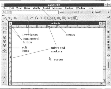
All CAD programs provide some useful aids to precise drawing. The Ortho option allows only horizontal and vertical lines to be drawn, no matter how the mouse is moved. This is useful for electronics diagrams in which lines representing connections are either horizontal or vertical. The Grid is a more generally useful guide to positioning the mouse, displaying a grid of faint dots on the screen. The spacing between the dots can be altered to a value that suits the drawing size; 1.0 mm is often useful for electronics work. The Grid is a guide, showing more clearly how far you have moved the cursor, and allowing you to move parts of a drawing into their correct positions, or draw them to correct dimensions.
An Attach option allows you to place either end of a line precisely, something that is not possible simply by moving the mouse. It may need to be switched off if you want to draw lines to or from points other than the ends or middle of another line, for example. Snaps are used to enforce precision of placing the cursor. When Snaps are selected the cursor can be moved only to snap points, which, if you are working with Grid on, will be the same as the grid size so that your cursor will snap to each grid point.
Your first requirement is to create or buy a set of electronics symbols. If you create your own, you need to work with care to ensure that the size of each component is suitable and that its terminals are on snap points, something that is not always easy for some shapes like transistors and inductors. Unless you have time on your hands, it is often better to buy a set of these sub-drawings. For each shape, whether a small part or a complete drawing, you can rotate, mirror-image and scale the drawings.
An object that is needed in many drawings can be saved as a Part, with some point of the object designated as the Part Base, a point for manipulating the object. The object can be drawn alone, with nothing else on the screen, and saved in the usual way, or it can be a portion of a larger drawing and saved using the Part Clip action. When the Part is needed, the Part option from the Draw menu is selected. This gives a list of all files, with small image (icons) to make selection easier. When the Part is loaded it can be moved to any part of a new drawing.
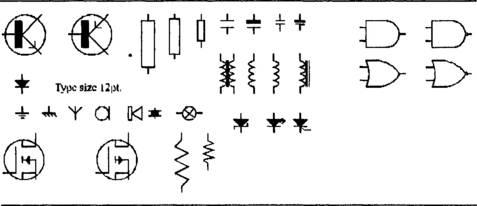
A simple way of creating a collection of Electronics Parts is to draw a circuit with as many types of components as possible, and save each component as a Part Clip. Even better is to collect a number together and save them as a file, Figure 10.2, which can be recalled when you want to create a circuit diagram. The illustration has been taken from the screen, and the printed version of these components is very much better than the screen version because of the limited resolution of the screen.
Any portion of a drawing can be selected so that it can be moved, copied, stretched, or have lines selectively broken. Move and Copy both make a new copy of an object at another position, but when Move has been selected, the original is deleted. This allows circuits to be built up by copying components from one place to another and then drawing in the connecting lines. The use of Snaps will ensure that all components are perfectly lined up and then the final work consists of copying over the round blobs that mark junctions in the circuit.
Zoomed views allow you to use the whole screen for a view of a drawing, or part of a drawing, at a different scale. This can be used to make the detail of part of a drawing more precise, or to make a small drawing fill the screen, or to make a drawing which is larger than the original limits fit into the screen space. This can be very useful if detail needs to be worked on, and it can be used in the opposite direction if the size of a drawing turns out to be larger than you expected.
Text can be added to any drawing, and the size of text characters is related to the drawing unit – this will almost always need to be changed. There are several sets of characters (or fonts); the default font provides characters that are drawn with simple straight-line strokes.
Because each drawing that is created by CAD methods can be saved as a disk file, it is often possible to make one drawing the basis of another, saving a considerable amount of work, and saving the new drawing under a different filename. Since no drawing need be committed to paper until it is needed, you can adjust as much as you like until the drawing is as you want it, something that is impossible when you work directly on to paper. In addition, where drawings make use of repetitive features (sets of IC pins, parallel lines of a bus, etc.) the multiple-copy actions make the creation of such shapes very fast and easy.
ELECTRONICS SPECIFIC PROGRAMS
The package referred to as Design Center or Eval Center contains a number of programs that are valuable for drawing and analysing circuits, passive or active. This package can be downloaded from a number of sites, notably
and various versions ranging from a simple Student version to a fairly full implementation can be obtained with no initial payment. The files are compressed (in Zip™ form) and your computer needs to be equipped with the WinZip™ or similar software to expand the files and install them. A particular advantage of using the package is that a drawing made using the Schematics option can then be analysed using the PSPICE option, with graphical output from the PROBE part of the package.
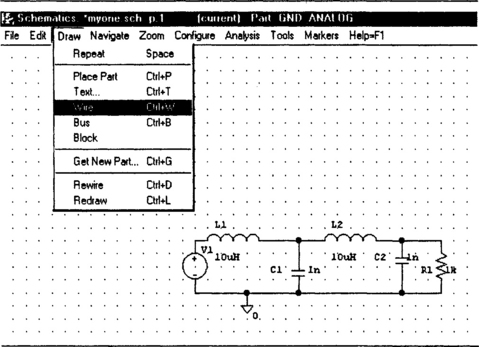
The drawing part of this set is titled Schematics, which is specifically intended for drawing electronics diagrams. When you opt to make a new drawing, you can select drawing units for a set of libraries called respectively, ABM, ANALOG, BREAKOUT, EXEL, PORT, SOURCE, SPECIAL, 7400 and FRQCHKX. You can use the Get New Part option from the Draw menu to select a unit from any of these. The drawing screen displays a set of grid dots, and any component you opt to place will move with the cursor until you click the mouse (a single click will place the item, allowing you to place another elsewhere, a double-click will place the item and end the action.
Figure 10.3 shows a sample drawing made in this way. The input has been selected from the SOURCE set, and the other components from the ANALOG set. The components are dragged into place, and snap to the nearest grid point when you click the (left-hand) mouse button. Each component can be moved by clicking and dragging, and the Draw—Wire command, illustrated, allows you to draw a wired connection together with a dot where one wire joins another.
You are not limited to US conventions (such as the zigzag resistor shape), because you can create symbols for yourself (after some practice) to add to the library. You can also change the default value that each component has as it is entered (such as 10k for a resistor or 1 nF for a capacitor) by editing each component in turn. The labelling as V1, C2, R3 and so on, is automatic, and you can determine what form of labelling you want. These features make the use of Schematics much more useful for electronics diagrams than CAD programs. In addition, a circuit created by using Schematics can be analysed by PSPICE and the graph of out/input (or other features) obtained using PROBE.
Linear circuit analysis
The analysis of linear circuits is based on the principles of the effect of resistive and reactive components on the amplitude and phase of a sine wave. For very simple circuits, this can be done either by drawing phasor diagrams to scale or by the use of algebra to express the circuit impedance as R + jX where X is the reactive component and j is the square root of minus one. These methods are comparatively simple but very tedious, and when the circuit is one that is only slightly more complicated than the most basic filter, the amount of work is enormously increased.
For many standard circuits, the formulae can be obtained from reference books (such as the splendid ITT Reference Data for Radio Engineers, now published by Howard Sams & Co. Inc. with the ISBN of 0-672-21218-2), but the amount of manipulation that is required becomes much greater, and in many cases you still have a lot of work to do after working out the results of each formula. The repetitive nature of the work, unless a programmable calculator is used, means that it is very easy to make mistakes.
When the circuit is not a standard one that can be looked up in a reference book, the analysis becomes very much more difficult. It amounts then to combining components, resistive or reactive, in series or in parallel, working out the first two, then combining with the next, and so on until the whole circuit has been covered. The aim is to express the effect of the whole circuit in the R + jX format so that the impedance magnitude (Z) is the square root of (R2 + X2) and the phase angle (φ) is the angle whose tangent is X/R. This analysis is long, tedious, and very liable to errors. It requires a good grasp of working with complex numbers (numbers including j) and for a large circuit the effort is very considerable. The working for a simple parallel resistor and capacitor will convince you, if you do not already know, that there is quite a lot of work involved.
Another dimension is added when a circuit contains one or more active components. The gain of an active component converts a passive circuit, whose power gain is always less than unity, into an active circuit which can have a power gain of more than unity over a considerable frequency range (the bandwidth). The gain–bandwidth product of the active device needs to be considered, however, as does the effect of the impedances of the active device.
None of this need be a problem for anyone with access to a PC-compatible computer because there are now several programs which ensure that even for very complex linear circuits, the effort of calculating frequency response can be performed by the computer. This brings linear circuit analysis, once possible only on very large and expensive computers, within the reach of any user, amateur or professional.
There are many linear analysis programs available at the time of writing, and if you use the Schematics portion of the PSPICE package the logical answer is to use PSPICE itself for analysis, and the companion PROBE for producing a graphical output. When you have a circuit diagram, with input and load, you can then produce an analysis, after saving the circuit as a file. The steps are:
You may find that the PSPICE step refuses to run, either because there is an error in the circuit (like no input) or because you have not specified the correct form of analysis (like AC sweep), or because you have not correctly specified the range of frequencies (PSPICE uses k for 1000 and MEG for 1 000 000 – a common fault is to use M, this means 10−3). Figure 10.4 shows a PROBE output graph for the circuit shown in Figure 10.3.
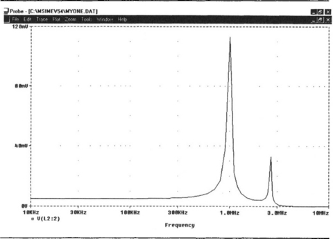
Figure 10.4 The graphical output for the circuit of Figure 10.3 taken at the output.
• Note that you can obtain an output at several designated points in a circuit. If your graph shows no changes, it may be because your designated point is the grounded end of a component.
The PSPICE package is ideal if you are using US conventions for circuit diagrams, but another analysis program that is particularly well suited for the small-scale UK user, professional or amateur, is called ACIRAN, and information is available from the website:
ACIRAN has been written by an engineer in the UK and is available in shareware form. For anyone not familiar with this way of distributing software, shareware programs are not obtainable in the usual way from computer shops but by downloading over the Internet and also from specialists in Public Domain and Shareware disks. Although most shareware programs originate in the USA, the ACIRAN program and one other linear analysis program have been written in the UK, so upgrades and support are more readily available.
In addition to its obvious applications to printing tables and graphs of response for a circuit, the use of the ACIRAN program makes it possible to allow for the effect of input and output impedances and of component tolerances, something that is particularly time consuming if done in the traditional ways. This is, however, the type of information that is particularly needed for small-scale production circuit design, so the use of methods based on the computer is a valuable aid to anyone involved in such work. In addition to the conventional R, C and L passive components, transmission lines can be dealt with, a considerable help to anyone involved in UHF design. As well as the built-in systems for dealing with transistors, FETs and op-amps, there is a current-generator component which can be used to simulate the action of any active components much more closely at high frequencies.
ACIRAN cannot be used until it has been notified of the circuit components and connections, and since ACIRAN cannot read a circuit diagram (although if circuit diagrams were prepared with standardized drafting programs such as ORCAD this could be done) it is necessary to use a system for entering the component positions and values. This system depends on identifying and numbering the circuit nodes, as you would when laying the circuit out for construction on PCB or stripboard.
Figure 10.5 shows a typical simple (in terms of components) passive circuit, with input and output and a common earth line, with nodes marked by numbers. A node, in this sense, means a point where components join, and this will normally include the input and the output as well as the earth (ground) connection. Each node can be numbered, and the convention followed by ACIRAN is that the earth (ground) node is always 0 (zero) and the input node is always 1. Other nodes can be numbered as you please, but it is better to take a logical arrangement of node numbers, moving from input to output.
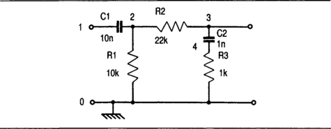
The general rule about nodes is that no node can have more than one number, and nodes are always separated by components. If there is no component between two nodes, one of the nodes must be redundant. If you need to work with nodes connected, use a small resistor value such as 0R33 between the nodes. You can use whatever number you like for the output node, because this will be notified to ACIRAN, but you must use the numbers 0 and 1 for the earth and input nodes respectively. Other linear analysis programs allow you to specify node numbers for all points, but this simply takes longer to set up; since every circuit will have an input and an output there is no reason why these should not be pre-allocated with node numbers.
The total number of nodes in this circuit example is five (numbered 0 to 4). There are also five components, but this is purely coincidental because the number of nodes does not depend in any simple way on the number of components. The point to watch in this illustration is the node numbered 4, because it is easy to overlook this one. Nodes where three or more components join are easy to spot on a well-drawn diagram because of the blob at the junctions, but this type of two-component junction is often less easy to see.
The form of the data can be seen in part in Figure 10.6, a view of the ACIRAN screen when the Data option of the menu has been selected. Small circuits can be checked from this display, but for a complex circuit it is better to print the data out and check against the circuit diagram, which should be numbered to show node positions. Once this set of data items has been entered, component values can be changed, but you cannot change the connections of a component. If you find, for example, that you have mistakenly entered R3 as lying between nodes 3 and 0 and wish to change this to nodes 4 and 0, you have to do this by deleting the component and re-entering R3 with its correct value between the correct nodes. The list will always show that a component has been deleted as a reminder of what you have done.

The form of entry of values follows the standard methods of specifying value, so that a figure by itself is taken to be in fundamental units of ohms, farads or henries. The suffix values of k, M, m, n, p and so on (lower case or capitals are taken as identical except for M and m) are all recognized, and you can enter values in the format 3K3 if you wish.
The analysis of this circuit is started with a wide frequency range and logarithmic response selected. This is always advisable so that the overall picture of the response can be seen, allowing you subsequently to change the frequency limits and sweep type if you want to see more detail. By specifying a large range initially, you ensure that the circuit has no surprises lurking outside the frequency range for which it is intended. This is unlikely in such a simple circuit, but the point about using ACIRAN is that it allows you to analyse circuits that are far from simple.
The table that appears following analysis takes the form shown in Figure 10.7 – this is only a part of the table as displayed on the screen. For each frequency in the range, the values of magnitude (amplitude), phase angle and time delay are printed, using units of decibels for amplitude, degrees for phase angle and seconds for time delay. The graph for amplitude is obtained by selecting Graph from the main menu, and appears, Figure 10.8, as the first of a set of at least three.


The other graphs are phase, Figure 10.9, and time delay, of which the time delay is usually of least interest for linear circuit work other than for specialized purposes. When options such as return loss and impedance values have been selected, there will be several more graphs of magnitude and phase angle for each of the other quantities covered.

PCB layouts
Programs for PCB layout have in the past been prohibitively expensive for the small-scale user, although some simplified systems for enthusiasts have been available for some time as shareware. Another choice that is particularly suited to UK professional users is from Number One Systems whose EASY-PC and EASY-PC Professional software is the leading software of this type in the UK. The address is:
Website: http://www.numberone.com
The EASY-PC program exists in two forms. The basic form allows you to draw circuit diagrams, linear or digital, using a set of ready-made symbol shapes that you can manipulate on screen and align with lines that are maintained straight and drawn horizontally, vertically or at 45°. You can, of course, add to the symbol library for yourself. The PCB layout can be drawn in the same way, using shapes that are the exact size of electronic components, along with pads and track lines. Although the PCB layout has to be drawn manually, you can manipulate it as much as you need before printing so as to ensure that the printout of the silk-screen view and of the copper track pattern will be perfect. Up to two silk screens and eight copper layers can be catered for.
The Professional version of EASY-PC allows the PCB connections to be drawn automatically after the circuit diagram has been drawn, and you can then arrange the components on the circuit board and re-route crossing tracks until the layout is satisfactory, with no need to specify each connection. The program can detect unwanted track crossings and points where there might be a danger of tracks shorting. In addition, when the schematic (circuit diagram) has been drawn using EASY-PC Professional, you can analyse the circuit action. Figure 10.10 illustrates a typical example of simple PCB layout.

Linear circuit analysis is carried out by the Analyzer software, providing graphs of amplitude and phase plotted against frequency and digital circuit analysis is carried out by the Pulsar software, providing simulated pulse inputs and showing, as if on a multi-track oscilloscope, output pulses. EASY-PC Professional contains both the Analyzer and Pulsar software, limited only in the number of components they can cope with, and you can upgrade if you need to analyse more elaborate circuits. Keep a close watch on the electronics press (or have your name added to the Number One Systems mailing list) to see upgrade offers.
This, along with the provision (also in EASY-PC) for multilayer boards and file output to Gerber Photo-plotting machines and to numerically controlled drilling machines, makes the professional version more suited for the designer of elaborate circuits who needs to design a large number of boards. Nevertheless, substantial numbers of hobby users of EASY-PC upgrade to the Professional version, and a brief description of this version is included in the book noted here.
For a full description of how to use EASY-PC, see the book (now out of print) The EASY-PC Handbook (Sinclair), ISBN 07506 2281 4 (Butterworth-Heinemann).