
Fundamentals
For many decades, engineers have been able to understand and apply electrical principles on the basis of treating electricity as a form of fluid, and quantities such as current remind us of this view. Electronics, however, often forces us to consider in more detail what electric current is as well as what it does. All of the effects that we describe as electrical or electronic depend on units of electrical charge called electrons.
For our purposes we can regard electrons as being particles of unimaginably small size, and all repelling each other. This force of repulsion exists over distances that are large compared to the apparent size of the electron, and we attribute it to a quantity called charge (or electric charge). Each electron appears to carry exactly the same amount of charge, and by convention we take the sign of this charge to be negative for an electron. A charge is positive if it attracts electrons, and the size of any charge is measured by the force which it can exert on another charge at a measured distance. Electrons are the outer parts of any atom, and when an electron is removed from an atom the atom is left with positive charge, as an ion, attracting the electron back to it. These forces are, however, greatly changed when atoms are closely packed together as they are in most metals, and the result is to release electrons, allowing them to take part in carrying current.
Electric current
These materials which conduct electric current well do so because they contain large numbers of electrons which are free to move, and it is this movement of electrons (or any other charged particles) that we call electric current. Conversely, insulators are materials which, although they may contain vast numbers of electrons, retain these electrons strongly bound to the atoms so that none of them is free to move and so carry current.
• Conduction in crystals can also be due to mobile defects in the crystal, called holes, but these exist only within the crystal and cannot have any independent existence.
For any material in which movement of electrons is possible, the number of electrons that passes a fixed point per second is a measure of the strength of the current. To put numbers to this, a current of 1 A is registered when 6.25 × 10¹² electrons pass per second – even this very small current demands that 6.25 million million electrons are moving past each second. In a good conductor, such as a metal, which contains vast numbers of free electrons, the average speed of the electrons is very low, of the order of a few centimetres per hour. In a poor conductor, such as a semiconductor material, the speed required for the same current would be considerably higher, measured in many centimetres per second.
• In a vacuum the electron speed is much higher, and it depends on the square root of the accelerating voltage. For example, in a cathode ray tube with accelerating voltage of 10 kV, the speed is around 60 million metres per second, but at 100 V acceleration the speed is around 6 million metres per second.
Since electric current is the movement of any particle that is charged, current flows when electrons move to and fro in a conductor, not only when the movement is in one direction only. Before anything was known of electrons, these two types of current were recognized and given the names AC (alternating current), and DC (direct current). In electronics, AC was at one time vastly more important, since all electronic signals consisted of AC, and DC was an incidental, used mainly for power supplies. Nowadays, many types of electronic signals consist of DC, so that we need to give equal weight to both of these types, although DC is often converted to AC so as to be more easily handled.
All electric current flows in a closed path, so that no atom is ever deprived of an electron because of the flow of electrons. An electron which leaves an atom will be replaced by an electron from another atom, so that electric current consists of a shuffling around of electrons, like musical chairs with no chairs being removed. The closer the chairs the less movement is needed, which is why the speed of electrons in a good conductor is low. Conversely, if the chairs are far apart, high speed is needed for the journey between chairs, corresponding to the high speeds of electrons in poor conductors.
Electrical quantities
The three electrical quantities that are of most interest to us are voltage, current and frequency. Current has been described already; it is the effect of the movement of electrons or other charged particles, and the strength of current is proportional to the amount of charge that passes a point per second. The voltage (more correctly potential, measured in units called volts) at a point is a comparative figure which measures the ‘pressure’ on electrons to move to or from that point to somewhere else. We usually take the potential (voltage) of the surface of the earth (a potential that is fairly constant) as that ‘somewhere else’, the zero level of potential, so that all voltages are measured by comparison to this zero, ground, or earth level. If the voltage of a point is such that electrons will flow to it from the earth, then that point has a positive voltage. Conversely, if electrons will flow from the point to earth, the point has a negative voltage. When the voltage at a point or the current in a circuit (a closed path) reverses at regular intervals then the voltage or the current is alternating, and the number of complete cycles of reversal (positive to negative to positive again, for example) per second is called the frequency.
The frequency of the AC power supply in the UK, and in most of Europe, is 50 Hz, where the hertz (abbreviated to Hz) is the unit of frequency that consists of one complete cycle per second. The standard frequency for North America is 60 Hz, and this has also been adopted for most of the American continent and in Japan.
• When a voltage is steady, it really ought to be referred to as ZF (zero frequency), because the term DC means direct current, and a phrase like DC voltage is really meaningless. A better choice would be constant current, but the use of DC voltage is now so common and so established that it has been followed in this book (and in most others) rather than the more appropriate ZF which could be applied to current or to voltage.
Active and passive components
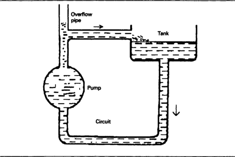
Electrical/electronic circuits consist of complete closed paths for current, starting at one end with a source of voltage (EMF) which uses energy to pump electrons around the circuit, and ending back at the source. The analogy with a water pumping circuit is very close (Figure 1.1), and extends to the idea that turning off a tap at the tank (breaking the circuit) will make the water level rise, because of the pressure of the pump, in a vertical piece of pipe (the voltage rises when the circuit is disconnected). Inside the source of EMF (electromotive force, an old term) energy of some sort is being used to push electrons around the circuit (when the circuit is connected) or to pile electrons up (when the circuit is disconnected).
Electronic circuits are built up by connecting components together with conducting paths which can be of metal wire, metal strips, or strips of other conducting materials such as doped silicon. In these paths, signals will be entering components and leaving components, and the power of a signal is measured by its voltage level multiplied by its current level. Electronic components generally are classed as being active or passive according to their effect on the power of signals applied to them. An active component can increase the power of a signal, using energy that is supplied in other ways, usually by a DC supply.
Passive components cannot increase the power of any signals applied to them and will almost inevitably cause power to be lost. Some passive components may increase the voltage of a signal, but this will be at the expense of current so that overall there is no gain of power. This definition is not totally watertight, because of the behaviour of varactor diodes and magnetic amplifiers, but is as near as we can get without becoming too elaborate at this stage.
A truly passive component can be used to reduce the power of a signal (deliberately), to select part of a signal by its voltage, its frequency or its time relationship to another signal, to change the shape of a waveform or to pass a signal from one section of a circuit to another; but in every case the power of the signal is decreased or unchanged, never increased. Resistors, capacitors and inductors are the fundamental passive components. There is a fourth type, however, called the gyrator, which is encountered in microwave circuits and which is of a more specialized nature.
An active component can increase the power of a signal and must be supplied both with the signal and a source of power. In many of the familiar active devices the source of power is a supply of current at a steady voltage, the DC supply, and the signal is fed in at one part of the active component and taken out from another. A few active devices have no separation of input and output, and some use an AC supply as the source of power and employ DC as their signals. The principle of using a power supply to increase the power of a signal, however, is unchanged.
An IC (integrated circuit) consists of a number of components, some purely active, some purely passive, others both active and passive, which are formed from the same materials, a semiconductor in single crystal or polysilicon ‘chip’ form. There may be terminals to this chip to which passive (or other active) components can be connected, but most of the circuit in the IC is inaccessible. Most ICs require a power supply, and are therefore classed as active components, and the advantage is that an IC can be treated as a single active component, with the reliability of a single component, whereas a circuit constructed from separate (discrete) components would contain huge quantities (ranging from thousands to millions) of components. This means that it would use a correspondingly large number of interconnections which would be considerably less reliable, since the reliability of a conventional circuit tends to decrease as the number of connections increases.
Thin-film circuits use techniques similar to those of IC manufacture in order to form passive components in miniature form, and thick-film circuits make use of materials other than semiconductors, such as metals that have been laid down by evaporation. Both thin-film and thick-film methods are used to make passive components for a variety of purposes.
Passive components
The fundamental main passive components are resistors, capacitors and inductors. The factor that they have in common is that they obstruct the flow of AC, although in very different ways, and are therefore said to present an impedance in the circuit. Resistors have a form of impedance which is termed resistance; and the effect of a resistance is to impede the flow of current equally for all frequencies of signal from DC upwards, although there are limits as we shall see later. In addition, when any current, AC or DC, flows through a resistor some of the energy of the current is converted to heat, causing the temperature of the resistor to increase. This heat is then passed on to the air (or anything else) that surrounds the resistor, and is a measure of the power that is being lost from the signal owing to the resistor. Wherever a resistor in a circuit passes current there will be a loss of power, and heat will have to be dissipated (usually to the air). The amount of heat will, however, be very small if the resistor is working at low voltage and current levels. At higher levels of power, if the heat is not dissipated, the temperature of the resistor will increase until the material melts or burns away. Usually this breaks the circuit, but for some resistor types it is possible for the material to fuse, decreasing the resistance, sometimes to short-circuit level.
Capacitors and inductors have reactance which, for a theoretically perfect capacitor or inductor, is not accompanied by resistance. Reactance also impedes the flow of current, but the amount of reactance is not a fixed quantity for one capacitor or inductor in the way that a resistor has a (more or less) fixed value of resistance. The reactance value of a capacitor or an inductor depends on the frequency of the current as well as on the component itself. At DC, capacitors have a very large reactance, amounting to complete insulation, and the size of the reactance decreases as the frequency of the signal is raised. Inductors have a very low reactance, almost zero for very low frequencies, but this value increases as the frequency of the signal is increased.
• The graph of reactance plotted against frequency for both capacitors and inductors will show minima and maxima due to self-resonance. An inductor will have self-capacitance and a capacitor will have some self-inductance, and in either case these will cause either series or parallel resonances.
When current passes through a pure reactance, high or low, no power is converted into heat and there is therefore no loss of power. In practice, no reactive component is perfect, although capacitors can come very close to the ideal, and any reactive component will have some resistance. When current passes, there will be a loss of power in this resistance, and the amount of such loss is expressed as a power factor (see later). The amount of loss should be very small for electronic components. Many circuits contain reactive components connected to resistors, and in such cases it is usual to assume that the power loss will be almost totally due to the resistor. Power loss in capacitors becomes significant for electrolytic capacitors subject to high ripple currents, and for other types mainly when signals of very high frequencies are applied.
The combination of resistance and reactance is known as impedance and the value of impedance for such a combination represents the total effect of resistance and reactance to an alternating current. We cannot calculate the value of impedance, however, by simply adding the value of resistance to the value of reactance. We have to find impedance in the same way as we can find distance between two points on a map when we have co-ordinates given. The similarity is illustrated in Figure 1.2, in which we map resistance, reactance (capacitive in this example) and impedance on a form of map called a phasor diagram. In this type of diagram, resistance values are always plotted along a horizontal scale and reactance on a vertical scale, down for capacitive reactance and up for inductive reactance.

Figure 1.2 A phasor diagram with reactance plotted vertically and resistance horizontally. The combination of reactance and resistance has impedance whose value can be measured from the diagram as the distance from the origin (point of zero resistance and reactance) to the point that represents the combination of resistance and reactance. Two points are shown here with impedance values of 5 and 13 respectively.
Why do we plot the reactance along a line which is at right angles to the line of resistance? If we connect a resistance and a reactance in series and we pass an alternating current through them both, then by using an oscilloscope we can detect something that ordinary meters will not show us. If the oscilloscope can display two traces together, we can use one trace to show the voltage across the resistor and the other trace to show the voltage across the reactive component. These traces (Figure 1.3) are always out of step with each other, and the amount of this displacement is one quarter of a cycle of the wave, so that one waveform is reaching a peak as the other passes through its zero level.
Now for any repetitive action, like the voltage in a wave, we can represent a cycle by a complete circle (Figure 1.4). The angle that a radius of a circle sweeps out for a complete circle is 360°, so that one quarter of a circle is represented by a rotation of 90°. For this reason, the displacement of one wave relative to the other of one quarter of a cycle is called a 90° phase shift, and this is the reason for the title phasor diagram and the drawing of the value of reactance as a line at right angles to the line that represents resistance value.
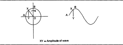
Figure 1.4 The connection between circular movement and a sine wave. The amplitude of the wave at any point corresponds to the distance from the horizontal axis of the circle to its rim for each point on the rim of the circle.
What is 90° out of phase in such a circuit is the current through the reactive component compared to its voltage. The voltage across a resistor can be used as a measure of the current that flows through it, because a resistor does not shift the phase of a current. A reactive component does shift the phase of current as compared to voltage, however, and always by 90°, so that by drawing a line to represent reactance at 90° to the line for resistance, we can complete the ‘mapping’ to obtain a value for impedance which is of both the correct size (represented by length of line) and phase angle (angle to the horizontal). This phase angle will be less than that for a reactive component by itself, but when more than one type of reactive component is present the phase angle of the resulting impedance can change considerably as frequency is changed.
Capacitors differ fundamentally from inductors in the direction of the phase angle. For a capacitor, the wave of current is 90° before the wave of voltage; for an inductor the wave of current is 90° after the wave of voltage. The easiest way to remember this is in the word C-I-V-I-L (C, I before V, V before I in L) in which the standard symbol letters of C for capacitor, L for inductor are used as well as I for current and V for voltage.
In addition to these fundamental (and traditional) passive components, the semiconductor diode is also considered as passive. It can be classed as a form of resistor with low reactance, but whose resistance value to current in one direction is vastly greater than the resistance value for current in the opposite direction. The arrow in the diode symbol (Figure 1.5) is used to show the direction of current for low resistance.

Basic electrical facts and laws
The basic facts and laws that relate to passive components are:
1. Ohm’s law, which states that for a metallic conductor at constant temperature, the resistance is constant. Since resistance is defined as the ratio of voltage across the component to current through it (Figure 1.6), Ohm’s law means that for most resistors, a value of resistance measured at one current is valid for any other current value providing the temperature of the resistor does not change appreciably.

Figure 1.6 Definition of resistance. This is not a statement of Ohm’s law, but our use of V = IR depends on Ohm’s law being obeyed.
2. Kirchhoff’s laws. The first law states that the current that leaves a circuit junction is equal to the current that enters it (conservation of current). The second law states that the sum of voltage across components in a circuit is equal to the circuit EMF (driving voltage). This is a law of conservation of voltage, and these two laws are simply another expression of the principle that electrons are never destroyed nor created. See Figure 1.7 for a diagrammatic explanation of these two laws.
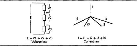
Figure 1.7 Kirchhoff’s laws, which mean that there can never be any current or voltage unaccounted for in a circuit.
3. The rules for addition of resistors or reactors in series and in parallel (Figure 1.8).

Figure 1.8 The rules for finding the effect of resistances, impedances and reactances in series and in parallel.
4. The rules for finding the reactance value of capacitors and inductors, and how these quantities vary with frequency of signal (Figure 1.9).

Figure 1.9 The formulae for reactance of capacitors and inductors, with tables of some values to show the effect of frequency. Note that reactance values for capacitors are negative (a consequence of the direction of phase shift).
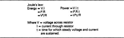
5. Joule’s law, which relates power dissipated by a resistive component with the current through the component and the voltage across it (Figure 1.10).
Note that most of these laws and rules apply irrespective of the frequency of the signal, and the only effect of signal frequency is on the reactance value of reactive components.
Waves and pulses
When a signal voltage varies from one instant of time to the next in such a way that its various voltage levels repeat at definite and fixed intervals of time, then we are dealing with a wave or a pulse. The difference between the two is that the voltage level of a pulse is steady for most of its cycle, with only brief intervals in which the voltage changes rapidly. By contrast, the voltage level of a wave is continually changing and will be steady only for very short time intervals (short compared to the time for a complete cycle). For others, such as square waves, the level can be steady for much of the time of a wave, but then changes abruptly.
Some types of waves and pulses are generated as the natural results of the laws of physics. For example, the sine wave is the result of rotating a coil in the field of a magnet, which is the principle of the alternator. A pulse is generated from a different type of action, the switching of a voltage on and off at regular intervals. Other forms of waves and pulses are not generated by any natural means, and in general all of the waveforms that are used in electronic circuits are generated by electronic methods rather than by ‘natural’ methods. There are obvious exceptions, such as the use of devices such as switches and tacho-generators, but most electronic waves are generated by electronic circuits called oscillators or function generators.
• Because the sine wave is mathematically the simplest waveform and is (approximately) the one that is conveniently supplied to us by the domestic electricity board, it has been customary in the past to think of it as the most important waveform and to regard it as the source of all others.
Mathematically, this is true because any other waveform (wave or pulse) can be constructed by adding a number, sometimes a vast number, of sine waves which have related frequencies but different voltages and phases. Today, however, electronics makes very considerable use of square waves and pulses, and in many ways it is easier to follow the principles of waves with reference to a square wave than to a sine wave. It is also much easier to draw square waves!
The square wave, which is the wave produced by repetitive switching, is shown in Figure 1.11, together with some of the terms that are used to specify and describe waveforms and pulses. The first point to note in the diagram is that there is a voltage baseline around which the square wave is symmetrical. This is shown as a dashed line which in this case lies midway between the extreme voltages of the wave.
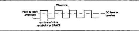
In many instances, this baseline is at ground voltage, but when it is not the wave is said to have a DC component whose size will be equal to the voltage between the baseline and ground voltage. This is the value which a moving-coil meter, or a digital voltmeter, set to a DC range would record if placed to measure voltage in the circuit, assuming that the presence of the meter did nothing to disturb the circuit conditions.
The amplitude of a waveform is a figure expressed in units of volts. It may be the peak amplitude, which is the voltage difference between the baseline and one voltage extreme of the wave, or the peak-to-peak voltage which is measured from one voltage extreme to the other. These peak and peak-to-peak amplitudes are not directly measurable by a meter, and would be obtained from oscilloscope readings.
The period (or wavetime) is the time in seconds (more usually milli-, micro- or nanoseconds) between one point on the waveform and the next identical point on the next wave. The most convenient point for this measurement is the point where the voltage is at the baseline value, and we must also specify the direction of movement of voltage (positive to negative or negative to positive). It can, however, be just as easily measured between any other recognizable points, such as the places where the voltage starts to change suddenly (Figure 1.12). Once again, this is a measurement that is often taken by an oscilloscope, although a digital frequency/period meter is also useful. Of the two, the digital measurement is likely to be considerably more precise if precision is required.
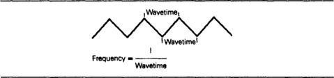
The inverse of period (1/period) when the period is expressed in seconds is frequency, and the unit is the Hertz, the number of waves per second. Frequency is measured directly by digital frequency meters, and period can be calculated from it (period = 1/frequency) rather than the other way round. The quantity which is actually measured depends on the instrument which is available; period if an oscilloscope is used; frequency if a digital frequency meter is used.
For some waveforms, particularly pulses, the width may be important. A pulse is a form of square wave in which the on time is much less than the off time (Figure 1.13) and for such a wave it is useful to know for how long the voltage is at the higher level, the on time. This figure of pulse width is then used along with the figure of frequency or time between pulses. Pulses are referred to as narrow or wide, according to the width, and in general a narrow pulse will have a width of 1 μs or less. For digital equipment, pulse widths are usually measured in nanoseconds rather than in microsecond units. A train of pulses is an asymmetrical waveform, so that the average DC value is not midway between the peaks (Figure 1.14).

Figure 1.13 The width of a pulse is the time for which the important part of the pulse is at a steady voltage.
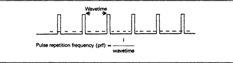
Figure 1.14 A train of pulses whose average value in this case is not zero – the average is marked by the dashed line.
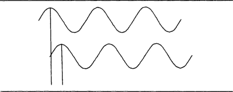
We can find that two square waves can have identical periods and amplitudes, but differ in time when they are displayed on a multiple-beam oscilloscope (Figure 1.15). The delay time is the difference in time between recognizable points such as the leading edges, the transition from negative to positive of each wave. This is the quantity that corresponds to phase shift of a sine wave, but the effects of the two have to be distinguished. The effect of delay on a square wave is simply to shift the time of the wave, preserving its shape. If there are phase shifts in a set of sine waves that make up a square wave, then unless the amount of phase shift is proportional to the frequency of each sine wave, the shape of the resulting wave will be changed.

Waveshape changes
The use of active components can carry out a large number of important changes to the shape of a waveform, but there are two particularly important changes which can be carried out by passive components, excluding diodes. These changes are called differentiation and integration and are particularly important when applied to pulse waveshapes. They are most easily described as they affect a waveform of square shape.
The square wave is made up of vertical (fast-changing) and horizontal (unchanging) portions. The effect of differentiation is to exaggerate the vertical portions and greatly reduce the amplitude of any horizontal portions. The overall amplitude may be greatly reduced during this process, so that differentiation often has to be followed by amplification. The effect of integration is to round off the vertical portions, smoothing out the waveform and reducing its amplitude so that, if carried to extremes, the output wave is almost DC (ZF), with just a slight trace of AC, called ‘ripple’. Of all waveforms, only a sine wave does not change shape when it passes through either of these networks, although there will be changes in both amplitude and phase.
The quantity that is important for the purpose of either differentiation or integration is called time constant, often abbreviated to τ (Greek letter tau) and measured in milli- or microseconds. Where the differentiation or integrating circuit is made up from a capacitor and a resistor, as is often the case, the time constant is found by multiplying the values of resistance and capacitance. Using units of capacitance in nanofarads and resistance in kilohms, the time constant will be in microseconds, and this set of units is usually more convenient than the textbook use of farads, ohms and seconds.
Suppose we imagine a capacitor connected in series with a resistor and a battery as shown in Figure 1.16. At the start, the capacitor is discharged and the battery is disconnected, so that the voltage across the capacitor is zero. What happens when the battery is connected? The answer is indicated in the graph – the capacitor will charge at a rate that starts fast but slows down as the charging proceeds. The shape of this graph is always the same, no matter what component values we use, but the amplitudes and time depend on the voltage of the supply and the values of resistance and capacitance that are used. The shape of the graph shows that the rate of charging decreases as the capacitor charges, so that, in theory, charging is never complete although for practical purposes the difference between the capacitor voltage and the supply voltage will be undetectable after some time. The simplest method of analysing what happens is by using the idea of time constant.
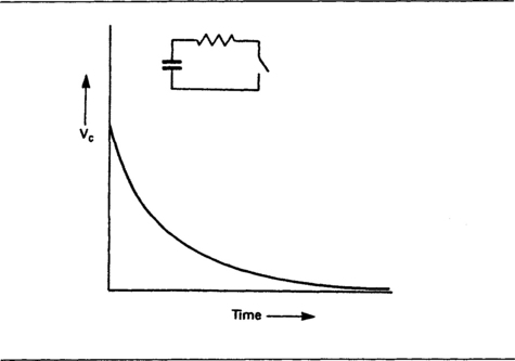
Figure 1.16 Capacitor charging. At the instant that the battery is connected, the capacitor starts to charge, but the charging is not instantaneous and is never totally complete.
The time constant corresponds to the time that the capacitor takes to be charged to a voltage level that is about 63% of the final voltage, the supply voltage in this example. This may appear to be a very awkward figure to choose, but it is not a chosen amount, it is the consequence of the shape of the graph for the charging capacitor. The significant point is that after another interval of time equal to one time constant, the capacitor will have charged to about 63% of the remaining voltage, which means to a level equal to about 77% of the final voltage. After a time equal to four times the time constant, a capacitor will have charged to about 98% of the final amount, so that for all practical purposes, we can say that the capacitor is fully charged. For more exacting purposes, a time of 6τ or 7τ may have to be used to provide an accuracy of 100 ppm.
When a charged capacitor is connected across a resistor, the capacitor will discharge, and the graph of voltage plotted against time for discharging is shown in Figure 1.17. Discharging follows the same pattern as charging, with about 63% of the voltage discharged in a time equal to a time constant. As before, then, we can take it for many purposes that a capacitor will be completely discharged in a time equal to four time constants.
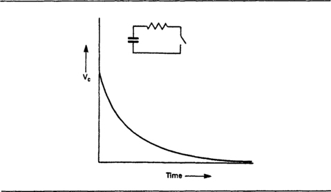
Figure 1.17 Capacitor discharging. At the instant that the switch is turned on, the capacitor starts to discharge, but this also is not instantaneous nor ever complete.
• Some types of capacitors, notably Mylar and high-K ceramic types, will need very much longer times for discharge because of voltage remanence or ‘soakage’ effects, see later.
The significance of these charging and discharging time constants becomes apparent when we want to find out the effect of a capacitor-resistor circuit on a signal that consists of a sudden change of voltage. Such a signal is called a voltage step, and signals of this type are used in all types of digital circuits, particularly in computer circuits. A voltage step is the leading or trailing edge of a square wave.
Figure 1.18 shows the shape of a voltage step from zero up to some fixed level, and the effect of the two possible simple capacitor-resistor circuits on this step. In each case, the waveform is the result of charging or discharging the capacitor, and the time that is needed is four time constants. In the first case (a), the capacitor is uncharged initially, so that each side is at the same voltage. After the step, however, the capacitor can charge, because one plate stays at the changed voltage and the other is free to pass current to ground through the resistor and so charge the capacitor. In the second case (b), the step voltage causes the capacitor to charge through the resistor until the voltage across the capacitor equals the voltage of the step.

Figure 1.18 A voltage step and its effect on two CR networks. (a) The capacitor starts discharged, so that the voltage across it is zero and all of the voltage is across the resistor, decreasing as the capacitor charges. (b) The capacitor again starts discharged, but the output now is across the capacitor and will rise as the capacitor charges.
These changes in waveshape may not necessarily be noticeable if the step up in voltage is followed by a step down, forming a square pulse. As Figure 1.19(a) shows, if the time between the step up and the step down is very short, much less than the time constant of the capacitor and the resistor, then the shape of the square pulse is almost unchanged. When shorter time constants are used, however, the shape of the pulse is considerably changed, and with very short time constants, the square pulse is transformed into two pulses, one corresponding to each voltage step. This action of a time constant that is short in comparison to the time of a square pulse is differentiation, and the resistor-capacitor circuit is a differentiating circuit.

Figure 1.19 The effect of the CR networks on a square wave, for a variety of values of time constant. In each set, the top waveform is obtained for a large value of time constant relative to period, the lowest waveform from a small value of time constant relative to period.
The integrator form of circuit, as illustrated in Figure 1.19(b), has very little effect on the square pulse if the time constant is very long compared to the time of the pulse. Using shorter time constants means that the capacitor is given less time to charge, so that the voltage never reaches the upper step level, and so the pulse is distorted into a slight rise and fall of voltage. Its effect is to smooth out a pulse, reducing the voltage step and extending the time. Both of these basic circuits are extremely important in all types of circuits that involve pulses, from TV circuitry to computer operation.
Differentiation and integration can also be unwanted effects. Sending a pulse through a long cable can have an integrating effect, smoothing out the pulse and spreading out the time for which the voltage changes. This effect was observed when the first transatlantic cables came into use, and was solved by matching the capacitance and inductance of the cable to resistors (terminating resistors) placed across each end. A properly matched cable will produce no integrating (or differentiating) effects. A full explanation of cable theory is beyond the scope of this book.
Undesired capacitance between two cables can result in a pulse on one cable producing a differentiated pulse on the other cable. In such examples, the capacitance is stray capacitance, and the resistance is the resistance that will exist in any circuit. One of the main problems in digital equipment is to maintain pulse shapes, particularly in a circuit that is physically large so that pulses have to travel along lines that are several centimetres in length. Many digital circuits make use of special circuits called drivers which are intended to reduce the problems of integration by supplying the pulse from a circuit that has very low resistance. This makes the time constant of this resistance with any stray capacitance very small, so as to have minimal effect on the pulse shape provided that the cable is correctly terminated. Once again, this topic is beyond the scope of this book.
Defects of square waves
We represent square waves on paper as being perfectly square, but a square wave, as examined by a good oscilloscope, may look anything but square. Some of the imperfections are due to the fact that the square wave must pass through networks (even if only the connections between the square-wave generator and the oscilloscope) which will differentiate or integrate the wave. Other imperfections are due to the generator itself, caused by the imperfect switching action of active devices. Figure 1.20 shows in detail some of the imperfections that may exist in a square wave, and the same terms are used to describe these faults in any type of pulse.

Figure 1.20 The imperfections that can exist in a square wave, caused mainly by stray capacitance and inductance.
The rise time measurement detects any integration of the wave. It is defined as the time taken for the voltage to rise from 10% of peak amplitude (measured from the base line, so that peak-to-peak is measured) to 90% of peak amplitude, expressed in microseconds or, more likely now, nanoseconds. The longer the rise time, the more the wave has been integrated, although square waves of very low frequencies can sometimes have quite long rise times (of the order of milliseconds) without detriment.
Overshoot is measured as the voltage of the overshoot peak as compared to the square wave high level, and is usually expressed as a percentage of that level. Overshoot is usually caused by inductance in the path of the wave, and is often followed by ringing, an oscillation of voltage which dies down after a few cycles. Both effects are very undesirable, and if inductance cannot be eliminated then it should be accompanied by enough resistance to ensure that the oscillation will be damped out even if the overshoot cannot be eliminated. In some cases, the overshoot will be due to inductance that has been added deliberately in order to improve the rise time of a circuit, and adjustment of the inductance value will be needed to ensure that the amount of overshoot and the rise time are both acceptable. When the overshoot is due to stray inductance, measuring the time of one cycle of overshoot can be a useful guide to estimating the amount of stray inductance.
The sag or droop of the wave is due to the presence of differentiating circuits in the wave path. A square wave of low frequency will have a flat top only if the circuit path is a DC path, containing no series capacitors and with no transformers used. At the higher frequencies, the differentiating effect of capacitors is less marked, but only a very small amount of differentiation is needed to produce a measurable amount of sag. Like overshoot, sag is quoted as a percentage of the normal steady high voltage level of the square wave.
The fall time, like the rise time, is measured as the time taken for the voltage to drop from the 90% level to the 10% level, and an extended fall time is also an indication that there is integration in the circuit. Many circuits use active devices in such a way as to make the rise time as short as possible, but with less attention paid to the fall time, so that it is normal to find that the fall time is greater than the rise time. A perfect square wave which has passed through totally passive circuits should have equal rise and fall times. Finally, the undershoot or backswing is measured and quoted in the same way as overshoot and may also be followed by ringing. This is less usual, even when inductance has been used to sharpen the rise time.
Metering and measuring
Practically all the applications for meters in electronics work are met either by some form of moving-coil meter or by a digital voltmeter. The moving-coil instrument consists of a magnet with pole-pieces shaped so as to generate a radial field (Figure 1.21) with a rectangular coil of wire suspended in the gap. The coil is supported by springs or by fine metal threads (in the taut-band version of the movement) which combine the actions of supporting the coil, passing current in and out, and restoring the coil to its rest position when it has been turned.
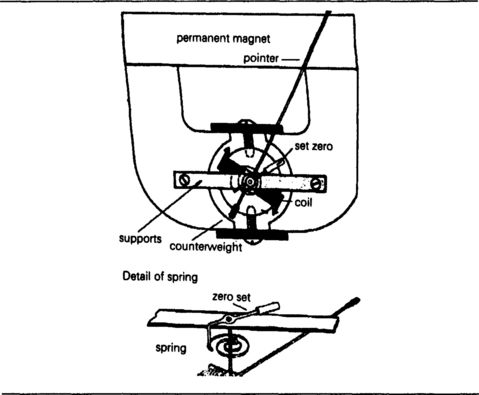
Figure 1.21 The moving-coil meter movement, which relies on current passing through a coil to move the coil in a magnetic field.
When current flows, the field of the magnet acts on the coil so as to turn it against the restoring torque (twisting effort) of the springs or threads. At some angle of turn the turning effort of the current equals the opposing effort of the springs, and the coil comes to rest so that a pointer attached to the coil will indicate a value on the scale of the meter. Typical sensitivities for modern instruments range from 1 μA to 50 μA for full-scale deflection (FSD), although movements in the 100 μA to 1 mA range are preferred for their low cost and rugged nature where the higher current is not a problem. In addition, the higher current movements have a lower resistance and a lower voltage drop across the movement at FSD.
Moving-coil instruments measure current, and any moving-coil movement will have its value of FSD current marked, along with the resistance of the coil. This allows the movement to be adapted to measure other current ranges and also to measure voltage and resistance. The other current ranges are obtained by using shunts, resistors of low value which take a known fraction of the current from the meter so that the range indicated is greater than the natural range of the movement. Voltage is measured by adding resistors in series to the movement so that the desired voltage range will pass the correct amount of current through the movement.
Figure 1.22 is a brief reminder of the methods that are used to calculate values of simple series and shunt resistor values, although most meters use a combination of series and shunt resistance.
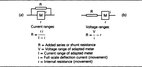
Figure 1.22 Extending the range of a current meter by adding shunt (a) and series (b) resistors to current and voltage ranges respectively.
Resistance is measured by a moving-coil meter by setting the meter to read full scale with a known resistance value in series with a battery, and then connecting in the unknown resistance so as to cause the current reading to drop. The scale that is used is non-linear and is a reverse scale with the zero resistance mark at the position of maximum current and voltage, and the infinite-resistance mark at the position of zero current or voltage.
• Some older moving-coil instruments pass enough current, when switched to a low-resistance scale, to burn out delicate components.
Digital voltmeters operate on an entirely different principle. Referring to the much-simplified diagram of Figure 1.23, the voltmeter contains a precision oscillator that provides a master pulse frequency. The pulses from this oscillator are controlled by a gate circuit, and can be connected to a counter. At the same time, the pulses are passed to an integrator circuit that will provide a steadily rising voltage from the pulses. When this voltage matches the input voltage exactly, the gate circuit is closed, and the count on the display represents the voltage level. For example, if the clock frequency were 1 kHz, then 1000 pulses could be used to represent 1 V and the resolution of the meter would be 1 part in 1000, although it would take 1 s to read 1 V. The ICs that are obtainable for digital voltmeters employ much faster clock rates, and repeat the measuring action several times per second, so that changing voltages can be measured. Complete meter modules are available, containing an IC, display and some passive components. The simple system illustrated here is very susceptible to noise pulses in the measured input, and in a practicable instrument the input would also be integrated to reduce this effect.
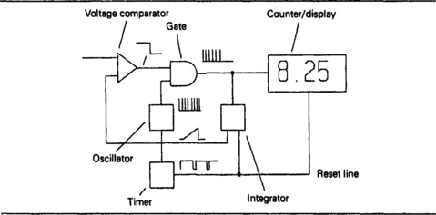
Figure 1.23 Principle of digital voltmeter. This depends on counting pulses that are added (integrated) until the resulting amplitude matches the input voltage.
• The example shows a type of circuit referred to as single slope, now obsolete. Modern digital voltmeters use a dual-slope action.
Like the moving-coil meter, the digital voltmeter can be adapted for other measurements. If the digital voltmeter is used, for example, to measure the (very small) voltage across a low-value resistor, then the meter can be scaled in terms of the current flowing, so that current measurements over a very wide range can be carried out. Resistance measurements are also possible, making use of a current regulator to pass a known current through the unknown resistor and measuring the voltage across the resistor. It is now possible to make at very low cost a digital meter whose precision is as good as the best moving-coil instruments of a decade ago, and the only penalty that is attached to the use of these instruments is that the reading can often take some time to settle down to a steady value, depending on the rate at which measurements are repeated.
Meter errors
There are two main sources of error in measurement made by any type of meter, the errors that are inherent in the meter itself, and those caused by adding the meter to a circuit. Of the two, the second type is often more important for moving-coil meters, because the precision of the meter is a known quantity (often 1 % or better), whereas the effect on the circuit has to be calculated or estimated.
There are two basic methods for measuring current in a circuit. One is to break the circuit so that the meter, moving-coil or digital, can be connected in series, set at the highest current range. The circuit is then switched on and the current range of the meter is adjusted until a useful reading (in the range of ![]() to
to ![]() full scale usually) is obtained. The alternative is to measure the voltage across a small resistor (1 Ω or less) which is permanently wired in series with the current circuit, so that a current measurement can be made without breaking any circuit. Either way, the resistance of the circuit is being changed by the addition of the meter.
full scale usually) is obtained. The alternative is to measure the voltage across a small resistor (1 Ω or less) which is permanently wired in series with the current circuit, so that a current measurement can be made without breaking any circuit. Either way, the resistance of the circuit is being changed by the addition of the meter.
The first method may be the only method available, but it is nearly always inconvenient to break the circuit, and it may be very undesirable to do so on a printed circuit board. In some circuits a clip-link may be provided so that current readings can be made easily. Such links can be placed at points in the circuit where the meter can be inserted without risk, because the insertion of a meter into points in the circuit where high-voltage pulses or large RF currents are present can cause damage to meters, and care must be taken to ensure that such waveforms do not pass through the meter. In general, a current meter should not be placed in any signal circuit. The arrangement of a permanent metering point in the form of a resistor in the current path is a better provision for current measurements, and if there is any possibility of unwanted signals the circuit can be arranged to ensure that these do not reach the meter by adding a bypass capacitor.
In general, inconvenient though the measurement of current may be, it disturbs a circuit much less than voltage measurement because the effect of current measurement is only to add a very small resistance in series with a circuit which will usually have a total resistance value that is very large in comparison. Voltage measurement using a moving-coil meter is much more likely to cause disturbance of circuit conditions. Although a voltage measurement is physically easy, involving clipping one meter lead to ground (or other reference point) and the other to the voltage point to be measured, the effect of the connection is to place the resistance of the voltmeter in parallel with the circuit resistance.
• This is no problem if a modern digital voltmeter with a very high input resistance (typically several kMΩ) is used, but older moving-coil instruments need to be used with considerable care.
Where the circuit resistances are high, comparable with the meter resistance, this can lead to readings which are quite unacceptably false. The meter reads as precisely as it can the voltage which exists, but this is not the voltage which would exist if the meter were not connected. The effect of a meter on a high-resistance circuit can be illustrated by considering a MOSFET circuit with a load resistor of 330 kΩ (Figure 1.24). Suppose that the meter is used on its 10 V scale, and that the MOSFET is cutoff so that the voltage ought to read 10 V. If the meter is made using a movement of 50 μA FSD, then for a 10 V reading on the 10 V scale, it would take 50 μA, so that the meter resistance is 200 k. The circuit, then, has now become a potential divider that uses a 330 k resistor (in the circuit) and a 200 k resistor (in the meter), and the voltage that now exists, and which is measured, will be 10 × 200/530 = 3.77 V.

Figure 1.24 The effect of current through a moving-coil meter can cause low readings when the current has flowed through a large resistor.
This is an exaggerated case, with an unusually high load resistance value, but it illustrates just how far out a moving-coil meter reading can be. There can be no confidence in a voltage reading, therefore, unless the meter resistance is known and is much greater (at least ten times greater) than the resistance through which current will flow to the meter. The resistance of a digital meter is usually high; older types used a fixed value of around 10 MΩ on all ranges, but modern instruments provide very much higher values, several thousands of MΩ in some cases. The resistance of a moving-coil meter depends on the range that is used, and can be calculated from the figure of merit that is written on the dial. This figure is shown as kilohms per volt, and the meter resistance is equal to this figure multiplied by the full-scale range. For example, if the meter figure is 100 kΩ per volt, corresponding to a 10 μA full-scale movement, then on the 10 V range the resistance is 100 × 10 = 1000 kΩ, which is 1 MΩ.
The use of the oscilloscope causes the same form of disturbance as the voltmeter, with the difference that the oscilloscope is used mainly on points in the circuit where signal voltages are present. The signal voltage is usually at relatively low impedance, so that the introduction of the oscilloscope has less direct effect because of resistance. The stray capacitance of the oscilloscope, however, can alter the signal conditions, and the input resistance of the oscilloscope can cause alterations in the DC conditions which might in turn alter the amplitude or waveshape of the signal (by altering bias, for example). Most modern oscilloscopes are DC coupled and although older types have input resistances of 2 MΩ to 5 MΩ, modern units (mostly of Japanese manufacture) have standardized the input resistance at 1 MΩ with a capacitance of 25 pF to 30 pF. This allows the use of standardized resistive or FET probes, so that a 9 MΩ resistor can be used in a 10 MΩ input probe, and FET probes can provide input resistance levels of 1000 MΩ or more along with very low capacitance.
Functions of passive components
Modern electronic circuits in general contain drastically fewer numbers of passive components than their counterparts of ten or fifteen years ago, but the part that these passive components play in the action of the circuit has become correspondingly more important. These actions include:
1. Setting levels of current and voltage for DC and for signals.
2. Selection of waveforms (tuning and filtering).
3. Alteration of waveforms (integration and differentiation).
All six are important. The trend in recent years has been away from the use of simple passive components in favour of more complex devices. One example is the use of electroacoustic filtering circuits in place of inductor–capacitor filters. This, however, has not affected the importance of the fundamental passive components, particularly resistors, which are now made in an even greater variety than ever existed earlier. The emphasis now is on the reliability of such components which has now become even more important since each passive component is of increased importance. In the chapters that follow, we shall examine passive components in turn, considering their action, construction, and the reasons for selecting one type rather than another.