
More Tips and Tricks for DSP Optimization
The first stage is getting the first 60–70% of optimization. This includes setting the right compiler switches to enable pipelining, keeping the loop from being disqualified, and other “simple” optimizations. This stage requires very basic knowledge of the architecture and compiler. By the end of this stage, the code should be running in real-time. This application note will provide the technical background and optimization tips needed to get to the end of the first stage of optimization.
The second stage is the last 30–40%. This stage requires an in-depth knowledge of how to interpret compiler feedback to reduce loop carried dependency bounds, reduce resource bounds, partition intelligently between inner and outer loop, and so on. Optimization at this stage may also require intelligent memory usage. In fact, the cache architecture of the DA6xx DSP may have a big impact on performance and should be considered when trying to optimize an algorithm fully. Optimal cache usage will not be addressed in this application note. However, there are many other papers on this topic. Please see the “References” section for pointers. This application note will not address techniques for second stage code optimizations either. However, references will be provided throughout this application note and in the “References” section on where to find more information on these second stage optimizations.
While any ANSI C code can run on a TI C6000 DSP, with the right compiler options and a little reorganization of the C code, big performance gains can be realized. For existing C code, one will need to retrofit the code with these quick optimizations to gain better performance. However, for new algorithm development, one should incorporate these optimizations into his/her “programming style,” thus eliminating at least one optimization step in the development cycle.
1.0 Software Development Cycle
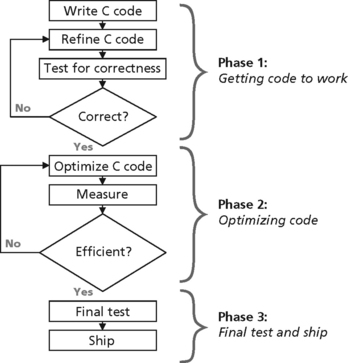
The concept of a software development cycle should not be new. The reason that it is mentioned explicitly here is to keep in mind that “getting code to work” and “optimizing code” are two very distinct steps and should not overlap. Optimization work should only begin after the code is working correctly.
In general, the compiler can be most aggressive when it does not have to retain any debug information. The C6000 compiler can be thought of having three aggressiveness levels that correspond to the three phases of software development.
In Phase 1, using appropriate compiler switches, the compiler should be set to its least aggressive setting. At this level, the compiler will perform no optimizations. Each line of C code will have corresponding assembly code, and the assembly code will be ordered in the same manner as the C source. This level of aggressiveness is appropriate when “getting the code to work.”
In Phase 2, using appropriate compiler switches, the compiler should be set to its mid aggressive setting. At this level, the compiler will perform many optimizations such as simplifying functions, eliminating unused assignments, converting arrays to pointers, and software pipelining loops (discussed later). The net result of these optimizations is assembly code that does not match with C source code line for line. This makes it more difficult to step through code or set breakpoints in C, for example, making debugging more difficult at this stage. Enough information is retained to profile on a function-by-function basis, however. Keep in mind that these optimizations do not alter the functionality of the original source code (assuming the original source is correct ANSI C and not relying on undefined behavior).
In Phase 3, using appropriate compiler switches, the compiler should be set to it most aggressive setting. At this level, the compiler has visibility into the entire program, across different functions and files. The compiler performs optimizations based on this program-wide knowledge, collapsing the output of multiple C source files into a single intermediate module. Only system-level debug and profiling can be performed at this stage, as the code will be reduced and reordered (depending on how much optimization was possible) such that it matches the C source in functionality only.
Note that after multiple iterations of C optimization, if the desired performance is still not achieved, the programmer has the option of using linear assembly. Linear assembly can be thought of as pseudo-assembly coding where the programmer uses assembly mnemonics but codes without immediate regard to some of the more complex aspects of the CPU architecture, that is, the programmer does not attend to scheduling of instructions. The compiler and assembly optimizer will manage the scheduling and optimization of the linear assembly code. In general, writing linear assembly is more tedious than writing C code but may produce slightly better performing code.
If the desired performance is still not achieved after linear assembly coding, the programmer has the option of hand coding and hand optimizing assembly code with no help from the compiler or assembly optimizer.
DSP Technical Overview
The CPU of the C6000 family of DSPs was developed concurrently with the C compiler. The CPU was developed in such a way that it was conducive to C programming, and the compiler was developed to maximally utilize the CPU resources. In order to understand how to optimize C code on a C6000 DSP, one needs to understand the building blocks of the CPU, the functional units, and the primary technique that the compiler uses to take advantage of the CPU architecture, software pipelining.
Functional Units
While thorough knowledge of the CPU and compiler is beneficial in writing fully optimized code, this requires at least a four-day workshop and a few weeks of hands-on experience. This section is no replacement for the myriad application notes and workshops on the subject (see Chapter 5.0 for references), but rather it is meant to provide enough information for the first round of optimization.
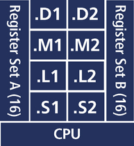
The CPU of the DA610 processor, in its most simplified form, looks like this:
Of course this diagram does not show all the memory buses and interconnects, but provides enough information for this discussion. The CPU has two sets of 4 distinct functional units and two sets of 16 (32-bit) registers. For the most part, each functional unit can execute a single instruction in a single cycle (there are a few exceptions). All functional units are independent, in other words, all functional units can operate in parallel. Therefore, the ideal utilization is all eight units executing on every cycle. (The memory architecture and CPU are organized such that eight instructions can be fetched and fed to the CPU on every cycle.)
The goal of the compiler is to reach ideal utilization of eight instructions per cycle. The goal of the programmer is to organize code and provide information to the compiler to help the compiler reach its goal. The programmer will achieve his/her goal by using appropriate compiler switches and structuring C code to exploit the powerful CPU. The Optimization Techniques section of this document will discuss such compiler switches and C coding techniques.
What “function” does each functional unit perform?
Below is a simplified breakdown of the function of each functional unit (each functional unit can execute many more instructions than listed here, see Fig. B.2).
| Unit | Floating-point | Integer |
| M | Multiplies | Multiplies |
| L | Add/Conversion | Add/Compare |
| S | Compares/Reciprocal | Add/Shift |
| D | Load/Store | Add/Load/Store |
Look at the simple example of a dot product.
In simple C code, we could write this as:
int dotp(short *a, short *m, int count)
The DA610 has the ability to perform a sustained dual MAC operation on such a loop. For example, the pseudo-assembly code for such a loop could look like (In reality, the above C code would not generate the following assembly code as-is. This example is for illustrative purposes only.):
LDDW .D1 *a, A7:A6; double-word (64-bit) load of a[i] and a[i+1]
![]() LDDW .D2 *m, B7:B6; double-word (64-bit) load of m[i] and m[i+1]
LDDW .D2 *m, B7:B6; double-word (64-bit) load of m[i] and m[i+1]
![]() MPYSP .M1 A6, B6, A5; single-precision (32-bit) multiply of a[i]*m[i]
MPYSP .M1 A6, B6, A5; single-precision (32-bit) multiply of a[i]*m[i]
![]() MPYSP .M2 A7, B7, B5; single-precision (32-bit) multiply of
MPYSP .M2 A7, B7, B5; single-precision (32-bit) multiply of
![]() ADDSP .L1 A5, A8, A8; accumulate the even multiplies in register A8
ADDSP .L1 A5, A8, A8; accumulate the even multiplies in register A8
![]() ADDSP .L2 B5, B8, B8; accumulate the odd multiplies in register B8
ADDSP .L2 B5, B8, B8; accumulate the odd multiplies in register B8
![]() [A1] SUB.S1 A1, 1, A1; loop counter stored in A1, if (A1!=0), A1––
[A1] SUB.S1 A1, 1, A1; loop counter stored in A1, if (A1!=0), A1––
![]() [A1] B .S2 loop; if (A1!=0), branch back to beginning of loop
[A1] B .S2 loop; if (A1!=0), branch back to beginning of loop
The horizontal bars (![]() ) in the first column indicate that the instruction is executed in parallel with the instruction before. (In this case, all eight instructions are executed in parallel.) The second column contains the assembly mnemonic. The third column contains the functional unit used. The fourth column contains the operands for the instruction. The last column contains the comments preceded by a semi-colon (;). The square brackets ([]) indicate that the instruction is conditional on a register. For example, [A1] indicates that the instruction will only be executed if A1!=0. All instructions can be executed conditionally.
) in the first column indicate that the instruction is executed in parallel with the instruction before. (In this case, all eight instructions are executed in parallel.) The second column contains the assembly mnemonic. The third column contains the functional unit used. The fourth column contains the operands for the instruction. The last column contains the comments preceded by a semi-colon (;). The square brackets ([]) indicate that the instruction is conditional on a register. For example, [A1] indicates that the instruction will only be executed if A1!=0. All instructions can be executed conditionally.
From this example, it can be seen that the CPU has the capability of executing two single-precision (32-bit) floating-point multiplies, two single-precision (32-bit) floating-point additions, and some additional overhead instructions on each cycle. The .D functional units each have the ability to load 64 bits, or the equivalent of two single-precision (32-bit) floating-point elements, each cycle. The .M units each can execute a single-precision (32-bit) multiply each cycle. The .L units can each execute a single-precision (32-bit) add each cycle. The .S units can perform other operations such as flow control and loop decrement to help sustain maximum throughput.
Figure B.3 shows a comprehensive list of the instructions performed by each functional unit.
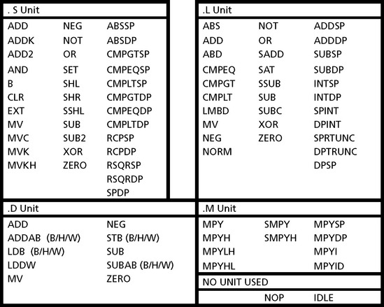
From Figure B.3, it can be seen that each functional unit can perform many operations and in some cases the same instruction can be executed in more than one type of unit. This provides the compiler with flexibility to schedule instructions. For example, the .S, .L, and .D units can each perform an ADD operation. Practically, this means that the CPU can execute six ADD operations, as well as two MPY operations, each cycle.
Software Pipelining
In most traditional DSP code, the majority of the cycles are in looped code, that is, contained in for() loops. This is especially true in audio DSP code where the algorithms are inherently block-oriented. Software pipelining is a technique that the compiler uses to optimize looped code to try to achieve maximum utilization of the CPU’s functional units. Software pipelining is enabled at the mid-level of compiler aggressiveness and higher.
Software pipelining is best illustrated by an example. (This example is not complete as it eliminates some concepts such as delay slots. It is meant to illustrate the concept of software pipelining only.)
How many cycles does it take to execute the following loop five times?
MPYSP; multiply two Single Precision (32-bit) floating point values
ADDSP; add two Single Precision (32-bit) floating point values
The parallel vertical bars (![]() ), at the beginning of line 2, indicate that the assembly instruction is executed in parallel with the instruction before. In this case, lines 1 and 2 are executed in parallel; in other words, two 32-bit values are loaded into the CPU on a single cycle.
), at the beginning of line 2, indicate that the assembly instruction is executed in parallel with the instruction before. In this case, lines 1 and 2 are executed in parallel; in other words, two 32-bit values are loaded into the CPU on a single cycle.
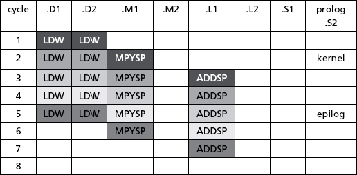
The following table illustrates the execution of this code withoutd software pipelining.
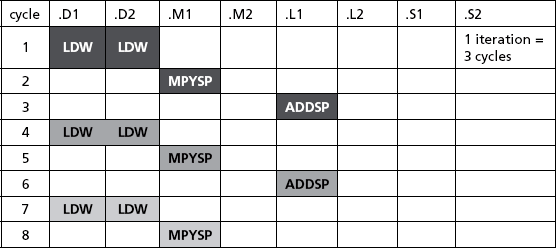
From the table, one iteration of the loop takes three cycles. Therefore five iterations of the loop will take 5 × 3 = 15 cycles.
By using software pipelining, the compiler tries to maximize utilization of the functional units on each cycle. For example, in some cases, the result of an instruction will not appear on the cycle following the instruction. It may not appear for two or three cycles. These cycles spent waiting for the result of an instruction are known as delay slots. Since the functional unit is not occupied during these “delay slots,” to maximize efficiency, the compiler will use these “delay slots” to execute other independent instructions.
Software pipelining can also be used if one part of an algorithm is not dependent on another part. For example, in looped code, if each iteration is independent of the previous, then the execution of the two iterations can overlap.
In this example, the delay slots are not shown, but we can still pipeline the code by overlapping execution of successive iterations. Since iteration 2 is not dependent on the completion of iteration 1, the CPU can start executing iteration 2 before iteration one is complete. Also, the CPU can start executing iteration 3 before iteration 2 and iteration 1 are complete, etc.
The following table illustrates the execution of this code with software pipelining.
From the table, the total execution time for five iterations is 7 cycles. By using software pipelining, the execution time was reduced by more than 50%. Also note that the execution time for six iterations is 8 cycles, i.e., each additional iteration costs only 1 cycle. For a large number of iterations, the average cost per iteration approaches one cycle.
A few terms need to be defined to discuss software pipelined loops:
Prolog: The overhead needed before the kernel can fill the pipeline.
Kernel: The core of the loop. In the kernel, the maximum number of functional units is utilized in parallel and the maximum number of iterations is being executed in parallel. In this example, in the kernel, four instructions are executed in parallel (LDW, LDW, MPYSP, ADDSP), four functional units are utilized at once (.D1, .D2, .M1, .L1), and three iterations of the loop are being executed in parallel. The kernel is executed over and over for most of the duration of the loop.
The number of cycles needed to execute one iteration of the kernel is called the iteration interval (ii). This term will appear again in the optimization section. In this example, each iteration of the kernel (LDW, LDW, MPYSP, ADDSP) executes in one cycle, so ii=1.
Epilog: The overhead at the end of a pipelined loop to empty out the pipeline.
To take advantage of the performance gains provided by software pipelining, the programmer needs to perform two important actions. First, software pipelining must be enabled through appropriate selection of compiler switches (explained in Optimization Techniques). Second, the C code within the for() loop needs to be structured such that the compiler is able to pipeline it. There are a few conditions that prevent certain code from being software pipelined. The programmer needs to make sure that the code is not “disqualified” from software pipelining (see section “Algorithm Specific Optimizations” for more information on software pipeline disqualification).
After the for() loop is able to be software pipelined, further optimization techniques will improve the performance of the software pipeline. This is also addressed in the section “Optimization Techniques.”
3.0 Optimization Techniques
At this point, the first phase of the development cycle should be complete. The algorithm has been designed, implemented in C, and tested for correctness. The code should work as expected, although maybe not as fast as expected. We are now ready to optimize. Until this point, during the “getting the code to work” phase, the lowest level of aggressiveness should have been used, that is, the only compiler switches selected should be −g and −k (and −ml0 to indicate far data model, to be safe).
-k keep generated assembly files
-ml0 far aggregate data memory model (to be safe)
(“Far aggregate data memory” model indicates that the entire .bss section is bigger than 32 kbytes. That is, the total space for all static and global data is more than 32 kbytes. If it is known that the .bss section is smaller than 32 kbytes, then the “near” data memory model should be indicated. The “near” data model is indicated by not using −ml at all. The “near” model uses a slightly more efficient manner to load data than the “far” model. If the “near” model is selected and the .bss section is actually bigger than 32k, an error will be flagged at build time.
Now, the functions that need to be optimized should be identified. These are the functions that consume the most cycles, or functions that need to meet critical deadlines. Within these critical functions, the main for() loop, that is, the most cycle intensive for() loop, should be identified. (There are many sophisticated profiling methods enabled by Code Composer Studio but are beyond the scope of this document. Please see Code Composer Studio User’s Guide, spru328 for more information on profiling.) Optimization effort should focus on this for() loop. Two things need to be done before optimization, a baseline cycle count needs to be obtained, and a simple test for correctness needs to be developed.
Get a baseline cycle count
Cycles will be the metric we use to measure how well optimized the code is. One can measure the cycle count of a particular loop without ever running code. This is a very crude way of measurement, but allows us a quick way of gauging optimization effort without the need for hardware or simulator.
Assume that the loop to be optimized is in function func() which is in a file foo.c. The compiler will produce a file (assuming −k option is selected) named foo.asm. In foo.asm, one can scroll down to _func to find the assembly version of func().
Under _func, in foo.asm, there will be a message such as:
;*----------------------------------------------------------------------------*
;* SOFTWARE PIPELINE INFORMATION
;* Disqualified loop: software pipelining disabled
;*----------------------------------------------------------------------------*
This is the beginning of the for() loop. Count the number of cycles between here and the comment:
which marks the end of the loop. Remember that parallel instructions count as one cycle, and NOP x counts as x cycles.
Many other sophisticated techniques exist in Code Composer Studio for profiling code. They are beyond the scope of this document.
Develop a test for “correctness”
When the mid and high levels of aggressiveness are used, the compiler will aggressively optimize the code using techniques such as removing unused functions, removing unused variables, and simplifying instructions. In some cases, improperly written code may be strictly interpreted by the compiler producing incorrect results. For example, a global variable may be tested in a loop in one file, but may be set elsewhere in the program (in an interrupt handler for example). “When the compiler optimizes the loop, it will assume that the variable stays constant for the life of the loop and eliminate the read and test of that variable, unless the variable is marked with the “volatile” keyword.
To catch such problems, a sanity check—whatever test makes sense for the system under development—should be run after each round of optimization.
Compiler Optimizations
These optimizations are not algorithm specific. They can be applied equally to all code.
Tip: Set mid-level aggressiveness
To set mid-level aggressiveness, change the –g option to −gp, add the −o3 option, and retain the −k option. At this level of aggressiveness, the compiler attempts to software pipeline the loop. The −k option has nothing to do with compiler aggressiveness, it just tells the compiler to save the intermediate assembly files. We will need this for the “Software Pipeline Information” feedback.
(See the beginning of Optimizing Techniques for an explanation of −ml.)
Use a profiling method for measuring the optimization gain. The simple technique mentioned above, opening the .asm file and counting cycles, is acceptable. Compare this cycle count to the baseline count.
C Code Optimizations
At this point, looking in the assembly output of the compiler (e.g., foo.asm), we should see one of two possible comments at the beginning of the for() loop:
;*––––––––––––––––––––––––––––––––––––––––––––––––––––––––––––––––––––––––––––*
;* SOFTWARE PIPELINE INFORMATION
;*––––––––––––––––––––––––––––––––––––––––––––––––––––––––––––––––––––––––––––*
;*––––––––––––––––––––––––––––––––––––––––––––––––––––––––––––––––––––––––––––*
;* SOFTWARE PIPELINE INFORMATION
;* Loop opening brace source line : 42
;* Loop closing brace source line : 58
;* Known Minimum Trip Count : 1
;* Known Maximum Trip Count : 65536
;* Known Max Trip Count Factor : 1
;* Loop Carried Dependency Bound(![]() ) : 14
) : 14
;* Unpartitioned Resource Bound : 4
;* Partitioned Resource Bound(*) : 4
If A is observed, the for() was disqualified from software pipelining, i.e., the compiler did not even attempt to pipeline the loop. If B is observed, the for() loop was not disqualified from software pipelining, i.e., the compiler did attempt to pipeline the loop. It is not necessary to understand the contents of B at this point (this is explained below). It is enough to know that if B is observed, the loop was not disqualified. Without some prior knowledge of the TI C compiler, it is not uncommon for A to occur.
If A is observed, it means the compiler tried to software pipeline the loop in question, but some code structure prevented it from being pipelined. There are a few reasons why a loop would be disqualified from software pipelining (for more information, see spru187). Below are a few of the more common reasons.
Loop contains a call: If there is a function call in the loop, and the compiler cannot inline that function, the loop will be disqualified.
Bad loop structure: Examples of bad loop structure are:
– Assembly statement within the C loop using “asm()” (intrinsics are OK)
– GOTO statements within the loop
– break statements within the loop
– Complex condition code requiring more than five condition registers.
Software pipelining disabled: Pipelining is disabled by a compiler switch. Pipelining is disabled if the −mu option is selected, if −o2 or −o3 is not selected, or if −ms2 or −ms3 is selected.
Too many instructions: Too many instructions in the loop to software pipeline. This is a problem because this code usually requires simultaneous use of more registers than are available. A workaround may be to divide the loop into consecutive smaller loops or use intrinsics (see explanation of intrinsics in the section Tip: Use intrinsics).
Uninitialized trip counter: The compiler could not conclusively identify the initialization instructions for the trip counter (loop counter).
Suppressed to prevent code expansion: If using the −ms1 option or higher, the compiler will be less aggressive about trading off code size for speed. In the cases where software pipelining increases code size with not much gain in speed, software pipelining is disabled to prevent code expansion. To always enable pipelining, use −ms0 option or do not use −ms option at all.
Loop carried dependence bound too large: A loop carried dependence is any dependence a later loop iteration has on an earlier iteration. The loop carried dependence bound is the minimum number of cycles between the start of iteration “n” of a loop and iteration “n+1” of a loop due to dependences between the two iterations.
If the compiler detects that a loop carried dependence is large enough that it cannot overlap multiple loop iterations in a software pipeline, then it will disqualify the loop from pipelining. Software pipelining cannot improve the performance of the loop due to the dependence.
The most likely (but not the only) cause of this problem is a “memory alias” dependence between a load instruction near the top of the loop and a store instruction near the bottom. Using the “restrict” keyword judiciously can help.
Cannot identify trip counter: This message indicates that the trip counter could not be identified or was used incorrectly in the loop body. The loop counter should not be modified in the body of the loop.
Tip: Remove function calls from within a loop
Function calls from within for() loops are the most common reason for pipeline disqualification in audio DSP code, therefore this should be the first thing to look for when a loop is disqualified from software pipelining. Removing function calls may sound simple, but there may be a few tricky situations.
At first pass, remove all the obvious calls like printf()’s or calls to other user functions. One way to eliminate debug calls like printf()’s is to save the information into temporary variables and then print them out at a future time.
Another way of eliminating the prinf() calls is to guard them with an #ifdef or wrap them in a macro. For example, the following macro can be used:
To use this macro, write your printf’s as follows (note the double parentheses):
dprintf((“Iterations %2d: x=%.8X y=%.8X ”, i, x, y));
If the code is compiled with a –dDEBUG compiler switch, then the printf is enabled. Without it, the printf disappears.
To eliminate calls to other (possibly user-defined) functions, try and inline the called function into the calling function.
One nonobvious function call that may be in the loop is a call to the modulo operator, %. When writing audio DSP code, use of circular buffers is common. Programmers unfamiliar with TI DSPs may be tempted to use the modulo operator to perform circular buffer addressing. For example, to update the index of a circular buffer, one may write:
sample = circ_buffer[index]; /* access the circular buffer via index */
index = (index + step) % circ_buffer_size; /* update the pointer */
In most cases, this syntax will be perfectly acceptable. (Please see section, TIP: Address circular buffers intelligently, for more details on circular buffer addressing techniques.) However, in a few cases, this syntax will produce less efficient code. In particular, when the argument of the modulo operator, in this case ‘circ_buffer_size’, is variable, then the modulo operator (%) will trigger a call to the run-time support (RTS) library to perform the modulo operation. This function call will disqualify the loop from software pipelining. For suggestions on what to put in place of the modulo operator, please see the section, TIP: Address circular buffers intelligently.
Other nonobvious function calls are: division by a variable, structure assignment (such as doing “x=y” where x is a “struct foo”), and long->float or float->long type conversion.
After removing all the function calls, the loop should now be qualified for software pipelining. This can be verified by looking in the assembly output file for the comments such as B above. If the loop is still disqualified, check the other causes for pipeline disqualification listed above. If the code is successfully qualified, measure the cycle count again to see the performance improvement.
Tip: Address circular buffers intelligently
Use of circular buffers in audio DSP algorithms is quite common. Unfortunately, when programming in C on a DA6xx DSP, the circular buffer addressing hardware is not accessible to the programmer. (When programming in assembly, this circular buffer addressing hardware is available.) This forces the programmer to manually check the buffer index for “end of buffer” conditions and to wrap that pointer back to the beginning of the buffer. Although this results in a little extra work on the part of the programmer (an extra one or two lines of code vs. using circular addressing hardware), the good news is that when done carefully, this manual manipulation of the buffer index will achieve the same performance as circular addressing hardware in most cases.
A typical line of audio DSP code using circular addressing hardware would look something like this:
sum += circ_buffer[index += step];
As “index” is advanced by an amount of “step,” the circular buffer addressing hardware would take care of wrapping “index” around back to the beginning of the buffer. Of course, prior to this line of code, the circular addressing hardware would need to be programmed with the buffer size.
On a TI DSP, to achieve the same functionality, the programmer would need an extra line or two of code. There are a number of different ways of writing the code to take care of wrapping the pointer back to the beginning of the circular buffer. Some are more efficient than others depending on the circumstances.
The most efficient way to write this code on a TI DSP would be:
index = (index + step) % size;
“size” is the length of the circular buffer.
As can be seen, only one extra line of source code was added from the first case. There are a few restrictions to writing the code in this manner in order to gain maximum efficiency from the compiler.
– “size” must be a constant (cannot be variable).
– “size” must be a power of 2.
– “step” and “size” must both be positive integers with ‘step’ < “size”
– The compiler knows that the initial value for “index” is 0 <= “index” < “size.”
The first two points are fairly straightforward, but the last point may need more explanation. It is very probable that the starting value for index will be in the range of 0 <= “index” < “size,” but how to inform the compiler of this fact?
This is done through an intrinsic called _nassert(). More information on _nassert() can be found in the section “Tip: Use _nassert().” For now, it is enough to know that_nassert() is only used to provide information to the compiler and does not generate any code. In this case, we need to inform the compiler about the initial value of “index.” At some point in the code, before “index” is used (in a loop) as in the example above, it must be initialized. At this point, _nassert() is used to inform the compiler of that initial value. The syntax would look like this:
_nassert(startingIndex >= 0); // inform compiler that initial value of
index = startingIndex % size; // set ‘index’ to its initial value
for (i=0; i<loop_count; i++) {
index = (index + step) % size;
Of course, this code is most efficient if the conditions are met. In some cases, the conditions may not be met, especially the first two. There may be a case where ‘size’ is not a constant or “size” is not a power of 2. In this case, use of the modulo operator (%) is not recommended. In fact, if these two conditions are not met, the modulo operator will actually trigger a call to the run-time support (RTS) library, thereby disqualifying the loop from software pipelining (see section “Tip: Remove function calls from within a “loop” for more information). In this case, an alternative is needed for updating the circular buffer index.
If the modulo operator (%) cannot be used because the conditions are not met, then the following code should be used to update the circular buffer index:
Although this code may seem inefficient at first glance, it is only three extra lines of C source code compared to the case where circular buffer addressing hardware is used. In those extra three lines of code, the operations performed are 1 ADD, 1 COMPARE, and 1 SUB. Recall from the section “Functional Units” that the ADD and SUB instructions can each be executed on any one of six different functional units (L, S, or D units on either side of CPU). Also, the COMPARE can be done on any one of two units (L units on either side of CPU). Thus, these three extra instructions can easily be executed in parallel with other instructions in the for() loop including any MPY instructions.
The net result is that updating the index of the circular buffer manually adds none to very little overhead vs. using circular addressing hardware. This is true despite the fact that a few more lines of source code are required.
Tip: More C code does not always produce less efficient assembly code
Since the CPU functional units are independent, when code is broken down into atomic operations, the compiler has maximum flexibility as to when to schedule an operation and on which functional unit. In the example above, a complex operation such as modulo with a variable argument could be reduced to three atomic operations, add, compare, and zero. This allowed the compiler to produce much more efficient code.
At this point, we need to learn a little bit about how to read the Software Pipeline Information. Here is an example:
;*----------------------------------------------------------------------------*
;* SOFTWARE PIPELINE INFORMATION
2 ;* Loop opening brace source line : 52
3 ;* Loop closing brace source line : 70
4 ;* Known Minimum Trip Count : 1
5 ;* Known Maximum Trip Count : 65536
6 ;* Known Max Trip Count Factor : 1
7 ;* Loop Carried Dependency Bound(![]() ) : 17
) : 17
8 ;* Unpartitioned Resource Bound : 4
9 ;* Partitioned Resource Bound(*) : 4
19 ;* Logical ops (.LS) 0 0 (.L or .S unit)
20 ;* Addition ops (.LSD) 6 1 (.L or .S or .D unit)
22 ;* Bound(.L .S .D .LS .LSD) 4* 3
24 ;* Searching for software pipeline schedule at …
25 ;* ii = 17 Schedule found with 3 iterations in parallel
28 ;* Collapsed epilog stages : 2
29 ;* Prolog not entirely removed
30 ;* Collapsed prolog stages : 1
32 ;* Minimum required memory pad : 0 bytes
34 ;* For further improvement on this loop, try option -mh2
36 ;* Minimum safe trip count : 1
37 ;*----------------------------------------------------------------------------*
Lines 1–3: Information on where the C code is located.
Lines 4–6: Information compiler has on number of times the loop is executed. This is important because the more information the compiler has on the loop count (trip count), the more aggressively it can perform optimizations such as loop unrolling. In this example, the compiler has no information on the loop count other than it will run at least once and at most 2![]() 16 times.
16 times.
If some information on the loop counter for any particular loop is known by the programmer, but not by the compiler, it is useful for the programmer to feed this information to the compiler. This can be done through the use of a #pragma. A #pragma is only used to provide information to the compiler. It does not produce any code. (For more information, see Tip: Use #pragma.)
Note that when the compiler is set to the highest level of optimization, it can usually figure out this loop count information on its own, without the use of a pragma. By examining lines 4-6, the programmer can determine if the compiler has enough information about the loop as it possibly could have. If not, then using a pragma is appropriate.
Line 7: This line measures the longest data dependence between consecutive loop iterations. This is important because the kernel of the loop could never be less than this number. The loop carried dependence constrains how aggressively multiple loop iterations can be overlapped due to dependences between the consecutive iterations. Instructions that are part of the loop carried bound are marked with the ![]() symbol in the assembly file.
symbol in the assembly file.
Lines 8–9: These lines indicate a limit (bound) on the minimum size of the kernel due to resource (functional units, data paths, etc.) constraints. “Unpartitioned”‘ indicates the total resource constraint, before the resources are assigned to the A side or B side of the CPU. ‘Partitioned’ indicates the resource constraint after the resources have been allocated to either the A or B side. This is important because the cycle count of the kernel of the loop can never be less than the larger of lines 8 and 9.
By comparing lines 8–9 (resource limitation) to line 7 (loop carried dependency limit), it can be quickly determined if the reduction in kernel size is limited by the resources used or the data dependencies in the loop. The bigger of the two is the limiting item. This helps guide further optimization efforts to either reduce resource usage or eliminate data dependencies.
Lines 10–22: These lines are a further elaboration on lines 8–9. Lines 10–22 show the actual usage for each resource on each iteration of the kernel. These lines provide a quick summary of which resources are used the most (thus causing a resource bound/limit) and which are under-utilized. If the kernel is resource constrained, optimization can be done to try and move operations from over-used resources to less used resources. The ‘*’ indicates the most-used resource, that is, the limiting resource.
.LS refers to operations that can be executed on either the L or S unit. Similarly, .LSD refers to operations that can be executed on each of the L, S, or D units.
“Bound (.L .S .LS)” is the resource bound value as determined by the number of instructions that use the L and S units. Bound(.L .S .LS) = ceil((.L + .S + .LS)/2).
“Bound (.L .S .D .LS .LSD)” is the resource bound value as determined by the number of instructions that use the L, S, and D units. Bound(.L .S .D .LS .LSD) = ceil((.L + .S + .D + .LS + .LSD)/3).
This information is useful if the iteration interval (ii) is limited by resources (not dependences). If this is the case, one should try to re-write code to use the unused resources and relieve the heavily used resources.
Line 25: ii is iteration interval. This is the length of the kernel in number of cycles. The kernel is the part of the loop that repeats over and over for the duration of the loop counter. It is where the bulk of the processing occurs.
In some cases, depending on the information provided to the compiler about the loop, the compiler may unroll the loop. When the loop is unrolled, one iteration of the kernel will execute multiple iterations of the original loop. For example, if the compiler unrolls the loop by a factor of 4, then each iteration of the kernel will execute 4 iterations of the original loop.
If a loop was unrolled by the compiler, a comment will appear within the Software Pipeline Information that looks like:
For large loop counts, one can calculate the approximate cycle time for one iteration of the original source loop by dividing ii by the loop unroll multiple. (In the case where the loop was not unrolled, the loop unroll multiple is 1.) So, ii/(loop unroll multiple) will approximate the number of cycles for each iteration of the original source loop, that is, the total cycle count of the for() loop will be approximately loop count * (ii/loop unroll multiple).
The goal in optimizing the loop is to make the kernel as small as possible, that is, make ii/loop unroll multiple as small as possible. By measuring ii after each optimization step, we will be able to gauge how well optimized the loop is.
Schedule found with 3 iterations in parallel means that on any iteration of the loop, before iteration n is completed, iteration n+1 and n+2 will have started.
Lines 28–30: As much as possible, the compiler will try to optimize for both code size and execution speed. To this end, the compiler can sometimes remove the prolog and/or epilog of the loop by executing the kernel more times (for prolog/epilog definition, see section on Software Pipelining). These lines indicate how successful the compiler was at trying to eliminate the prolog and epilog sections. No actions by the programmer are necessary based on information from these lines.
Line 32: Sometimes the compiler can reduce code size by eliminating the prolog and/or epilog and running the kernel more times. For example, if the epilog were removed, the kernel may run one or more extra iterations, but some of the results from the extra iterations may not be used. An extra memory pad may be required on the data buffer, both before and after the buffer, to guard against these “out-of-bounds” accesses. The data in the pad region will not be modified. This line in the pipeline feedback indicates how much of a memory pad is required. This technique is known as “speculative load.”
Note that on the DA610, the overflow part of the buffer (the memory pad) may not reside in L2 Cache. Incorrect behavior may result if it does. Buffers for loops in which the speculative load technique is used may only reside in L2SRAM and must be at least “memory pad” bytes away from the end of L2SRAM (and the beginning of L2 Cache). (See spru609 for more details on memory architecture.)
The “speculative load threshold” value is a measure of how aggressively the compiler uses this technique to collapse code. This speculative load threshold value can be adjusted with the −mh compiler option. If a memory pad were suggested for the loop, a second line of comment would have been added to inform the programmer of the minimum required threshold value to attain that level of collapse.
Line 34: This line provides an optimization suggestion in the form of a higher threshold value that may be used to cause even more collapsing of the loop.
Line 36: The minimum number of times the loop needs to run, that is, the minimum loop count, to guarantee correct results.
Tip: Mind your pointers
Inform the compiler as much as possible about the nature of pointers/arrays.
One easy C code optimization that can be done in accordance with this tip is to include the size of an array in a function declaration that uses that array as an argument, if the array size is known. For example, if it is known that the size of an array is always 256 elements, then a function declaration using this array would look like:
void function(int array[256]);
This helps the compiler improve its analysis of the function. In general, the compiler prefers to see array declarations, particularly when the size of the array is known.
Another C optimization in accordance with this tip occurs if there are two pointers passed into the same function. The compiler can better optimize if it knows if the two pointers could point to the same memory location or not.
Here is an example prototype for an audio algorithm:
void delay(short *inPtr, short *outPtr, short count)
The function is passed a pointer to the input buffer (inPtr) and a pointer to the output buffer (outPtr). This is common in audio algorithms. The algorithm will read data from the input buffer, process it, and write data to the output buffer.
With no additional information, the compiler must be conservative and assume that inPtr and outPtr access the same buffer, in other words, a write by one pointer can affect a read by the other pointer. The ‘restrict’ keyword can be used as a type qualifier on a pointer to guarantee to the compiler that, within the scope of the pointer declaration, the object pointed to can only be accessed by that pointer. This helps the compiler determine memory dependencies hence more aggressively optimize. The ‘restrict’ keyword can also be used with arrays.
In this case, using the ‘restrict’ keyword provides a guarantee to the compiler that inPtr and outPtr do not point to overlapping memory regions. Rewriting the above function with the ‘restrict’ keyword helps the compiler produce more optimized code:
void delay(short* restrict inPtr, short* restrict outPtr, short count)
Another problem that may occur with pointers is a little more subtle, but still common. What happens if the pointers are pointing to overlapped spaces, that is, two pointers do point to the same buffer? This is common in audio algorithms when using a delay buffer. One pointer may be reading from one part of the delay buffer while another pointer may be storing a value to another part of the buffer. For example,
delay_buffer[current] = constant * delay_buffer[old];
out[i] = in[i] + (gain * delay_buffer[old]);
From looking at the code, delay_buffer [old] could be read once and used in both lines of code. From our knowledge of the CPU, we would assume that delay_buffer[current] and out[i] could be calculated in parallel.
However, in this case, delay_buffer[current] and delay_buffer [old] physically exist the same buffer. Without any other information, the compiler has to be conservative and assume that there is a possibility of current ==old. In this case, the code could look like:
delay_buffer[old] = constant * delay_buffer[old];
out[i] = in[i] + (gain * delay_buffer[old]);
The result of the first line is used in the second line, which means that the second line can’t start executing until the first line finishes. If we can guarantee that current!=old always, then we need to specify this to the compiler so that it can be more aggressive and execute the two lines in parallel.
This is where the subtlety comes into play. If delay_buffer[old] and delay_buffer[current] never point to the same location for the entire duration of the function (ideal situation), then they should be passed into the function as two distinct pointers with one of them specified as “restrict.”
For example, if loop_count=100, and we know that (old > current+100), then delay_buffer[old] and delay_buffer[current] will never point to the same location fo the duration of loop_count. In this case, the declaration of the function should be:
void delay(int* restrict oldPtr, int* currentPtr, int count)
and the function should be called using the following:
delay(&(delay_buffer[old], &(delay_buffer[current], 100)
This will inform the compiler that the two pointers never point to the same memory location for the duration of the loop.
The second scenario (nonideal) is that we cannot guarantee that delay_buffer[old] and delay_buffer[current] will not point to the same memory location for the duration of the loop. However, if we can guarantee that they will not point to the same memory location for each iteration of the loop, then we can still optimize. In this situation, we do not modify function is defined, but we do modify the code slightly within the loop.
If we know that current! =old always for each iteration of the loop, then we could re-write the code this way:
float temp_delay; //define a temp variable for unchanging delay value
temp_delay = delay_buffer[old];
delay_buffer[current] = feedback * temp_delay;
out[i] = in[i] + (gain * temp_delay);
Now the compiler will produce code to execute the two lines in parallel.
Tip: Call a float a float
Floating-point constants are treated as double-precision (64-bit) unless specified as single-precision (32-bit). For example, 3.0 would be treated as a 64-bit constant while 3.0f or (float)3.0 would be treated as single-precision (32-bit).
One of the benefits of the DA610 is being able to write floating-point code. However, when using constants, one has to know how the compiler will interpret the number. In the C6000 family, the following names are used for floating-point data types:
float – (IEEE) 32-bit floating-point
double – (IEEE) 64-bit floating-point
Care needs to be taken when using floating-point constants. Look at the following lines of code.
In this example, the code has specified to the compiler that x and y are to be single precision (32-bit) floating-point values (by defining them as float), but what about M? All that is indicated to the compiler is that it is to be floating-point (by virtue of the decimal point), but we haven’t specified single-precision (32-bit) or double-precision (64-bit). As usual, without any information, the compiler will be conservative and assume double-precision.
The resulting assembly code from the above code will be:
![]() MVKH .S1 0x40100000,A1; put constant (4.0) into register A1
MVKH .S1 0x40100000,A1; put constant (4.0) into register A1
; A1:A0 form DP (64-bit) constant (4.0)
MVKH .S1 0x40400000,B4; put x (3.0) into register B4
SPDP .S2 B4,B5:B4; convert x to DP (64-bit)
MPYDP .M1X B5:B4,A1:A0,A1:A0; DP multiply of x (B5:B4) and M (A1:A0)
NOP 9; wait 9 delay slots for the multiply
DPSP .L1 A1:A0,A0; convert the DP (64-bit) result (y) to SP (32-bit)
This is more code than what would be expected for a 32 × 32 floating-point multiply. The problem is that even though a 32 × 32 multiply was intended, we did not inform the compiler of this. To correct the situation, indicate to the compiler that the constant is single-precision. There are two ways to do this:
#define M 4.0f // or (float)4.0
produces the following assembly output:
MVKH .S1 0x40400000,B4; move x (3.0) into register B4
MVKH .S1 0x40800000,A0; move M (4.0) into register A0
MPYSP .M2X B4,A0,B4; (single-precision) multiply of M*x
Making sure to specify constants as ‘float’, when single precision floating-point is desired, will save both code space and cycles.
In general, the programmer always has to be mindful of data types. Mixing floating-point and fixed-point data types in a calculation when not required will cause unnecessary overhead.
In this case, the compiler will treat C as a floating-point value but a and b are declared as fixed-point. This forces the compiler to add instructions to convert C from floating-point to fixed-point before doing the addition. Instead, the code should read:
Tip: Be careful with data types
The following labels are interpreted as follows by the C6000 compiler. Be careful to assign the types appropriately. Each of the following data types can be signed or unsigned.
| char | 8-bit fixed-point |
| short | 16-bit fixed-point |
| int | 32-bit fixed-point |
| long | 40-bit fixed-point |
| float | 32-bit floating-point |
| double | 64-bit floating-point |
Do not confuse the int and long types. The C6000 compiler uses long values for 40-bit operations. This may cause the generation of extra instructions, limit functional unit selection, and use extra registers.
Use the short data type for fixed-point multiplication inputs whenever possible because this data type provides the most efficient use of the 16-bit multiplier in the C6000 (1 cycle for “short * short” vs. 5 cycles for “int * int”).
Use int type for loop counters, rather than short data type, to avoid unnecessary sign-extension instructions.
Do not use unsigned integer types for loop counters or array subscript variables. i.e., use int instead of unsigned int.
When using floating–point instructions on a floating-point device, such as the C6700, use the -mv6700 compiler switch so the code generated will use the device’s floating-point hardware instead of performing the task with fixed-point hardware. For example, if the -mv6700 option is not used the RTS floating–point multiply function will be called instead of the MPYSP instruction. Specifically, the flag “−mv6710” should be used for DA6xx and C671x devices and “-mv6210” should be used for C621x devices.
Tip: Limit type conversions between fixed and floating-point
Any conversions from fixed-point to floating-point (e.g., short->float or int->float) or from floating-point to fixed-point (float->short or float->int) use the valuable L unit in the CPU. This is the same hardware unit that performs floating-point ADDs, for instance. Many type conversions along with many floating-point ADDs will over-stress the L unit.
If a variable needs to be converted from int to float, for example, and then will be used many times, convert the variable once and store in a temporary variable rather than converting on each usage.
Assume that part of the loop looks like the following:
void delay(short *in, short *out, int loop_count)
float feedback, gain, delay_value;
buffer[current] = (float)in[i] + feedback * delay_value ;
out[i] = (short)((float)in[i] + (gain * delay_value));
In this case, the arrays in[] and out[] both contain fixed-point values. Thus, in[i] needs to be converted to floating-point before being added to (floating-point) delay_value. This needs to be done twice, once for each ADD. It would be more efficient to do the conversion from fixed to floating-point once, then use that converted in value in both calculations. In other words, the more efficient way to code this would be:
void delay(short *in, short *out, unsigned short loop_count)
float feedback, gain, delay_value;
float temp_in; //temporary variable to store in[i] after conversion
temp_in = (float)in[i];//do the conversion once only
buffer[current] = temp_in + feedback * delay_value ;
Tip: Do not access global variables from within a for() loop
This is a general tip on C coding style that should be incorporated into the programmer’s programming style. If global variables need to be used in a for() loop, copy the variables into local variables before the loop and use the local variables in the loop. The values can be copied back to the global variables after the loop, if the values have changed. The assembler will always load global variables from the data pointer area, resulting in less efficient code.
Tip: Use #pragma
In some cases the programmer may have knowledge of certain variables that the compiler cannot determine on its own. In these cases, the programmer can feed information to the compiler through the use of #pragma. #pragma does not produce any code, it is simply a directive to the compiler to be used at compile time.
For example, for looped code, often the loop counter is passed in as a variable to the function that contains the looped code. In this case, the compiler may have difficulty determining any characteristics about the loop counter. The programmer can feed information about the loop counter to the compiler through the use of the MUST_ITERATE pragma.
#pragma MUST_ITERATE(min, max, factor)
min – minimum number of iterations possible for the loop to execute
max – maximum number of iterations possible for the loop to execute
factor – known factor for the loop counter, for example, if the loop will always run an even number of times, then factor could be set to 2.
It is not necessary to have all three pieces of information to use this pragma. Any of the arguments can be omitted. For example, if all that is known about a particular loop is that any time it runs, it will run for at least 4 iterations and it will always run an even number of iterations, then we can use the pragma in the following way:
This line says that the loop will run at least 4 times, and it will run an even number of times (i.e., 4, 6, 8, …). This line should be inserted immediately preceding the for() loop in the C source file.
Another use of #pragma is to direct the compiler to compile the code in a specific way. One of the more useful pragmas for looped code is the UNROLL pragma. This pragma specifies to the compiler how many times a loop should be unrolled. It is useful since the resources of the CPU can be spread over multiple interations of the loop, thereby utilizing the resources more efficiently.
For example, say that the original source code requires three multiplies for every iteration of the loop. Since there are two multiply hardware units, two cycles per iteration will be required to execute the three multiplies. If the loop were unrolled such that two iterations of the original source code were executed at once, we would be required to execute six multiplies per iteration. Since there are two multiply hardware units, three cycles would be required to execute the six multiplies. In other words, three cycles are required to execute two iterations of the original source code for an average of 1.5 cycles per iteration. By unrolling the loop by a factor of two, we have reduced the execution time from two cycles per iteration to 1.5 cycles per iteration.
A few things need to be considered when using this pragma. It will only work if the optimizer (−o1, −o2, or −o3) is invoked. The compiler has the option of ignoring this pragma. No statements (but other pragmas are ok) should come between this pragma and the beginning of the for() loop.
which indicates to the compiler that the loop should be unrolled by a factor of n. In other words, one iteration of the kernel should execute n iterations of the original loop.
To increase the chances that the loop is unrolled, the compiler needs to know the smallest possible number of iterations of the loop, the largest possible number of iterations of the loop, and that the loop will iterate a multiple of x times. The compiler may be able to figure out this information on its own, but the programmer can pass this information to the compiler through the use of the MUST_ITERATE pragma.
#pragma MUST_ITERATE(32, 256, 4)
for (i=0; i < loop_count; i++) …
These lines indicate that the loop will run at least 32 times and at most 256 times and that loop_count will be a multiple of four (32, 36, 40, …). This also indicates to the compiler that we want four iterations of the loop to run for every one iteration of the compiled loop, that is, we want the loop to be unrolled by a factor of 4.
Tip: Use _nassert()
The _nassert() intrinsic generates no code and tells the optimizer that the statement contained in its argument is true. This gives a hint to the optimizer as to what optimizations are valid.
A common use for _nassert() is to guarantee to the optimizer that a pointer or array has a certain alignment. The syntax for giving this pointer alignment is:
_nassert((int) pointer % alignment == 0);
For example, to inform the compiler that a pointer is aligned along an 8-byte boundary (“double-word aligned”):
_nassert((int) buffer_ptr % 8 == 0);
This intrinsic along with the MUST_ITERATE pragma gives the compiler a lot of knowledge to use when optimizing the loop.
In the use of _nassert(), one question may arise: How do we know that a pointer is aligned? The answer is that we can force the compiler to align data on certain boundaries by using the DATA_ALIGN pragma. The syntax for this pragma is:
#pragma DATA_ALIGN(symbol, constant);
In this case, “symbol” is the name of the array to be aligned and “constant” is the byte boundary to which it will be aligned. For example, to be aligned on a 16-bit (short or two-byte) boundary, we would use a constant of 2. This would guarantee that the first address of the array will be a multiple of 2 (in other words, the compiler will place the array such that the starting address is 0x0, or 0x2, or 0x4, .). To be aligned on a 64-bit (i.e., double-word or eight-byte) boundary, we would use a constant of 8. This would guarantee that the first address of the array will be a multiple of 8 (i.e., the compiler will place the array such that the starting address is 0x0 or 0x8 or 0x10 or 0x18, …). This pragma should be inserted directly before the declaration of the array. For example:
#pragma DATA_ALIGN(buffer, 8);
This will declare a buffer of size 256 floats (1024 bytes), and align this buffer to an 8-byte boundary. Now the _nassert intrinsic can be used to inform the compiler that ‘buffer’ is on a double-word boundary.
Tip: Get more feedback
Using −on2, the compiler produces an .nfo file. This file provides more information on advanced optimizations for getting better C performance. The suggestions will usually be in the form of different compiler switches, or additional compiler directives. If compiler directives are suggested, the .nfo file will show what code to include and where to include it in the C source file.
Other System Level Optimizations
There are some optimizations that are not necessarily for a specific loop but can help increase overall DSP performance.
Tip: Use Fast run-time support (RTS) library
The fast run-time support (RTS) library is a set of math functions provided by TI and optimized to run on TI’s floating-point DSPs. The FastRTS library implements functions such as arctangent, cos, sin, exponent (base e, 10, and 2), log (base e, 10, and 2), power, reciprocal, divide, and square root. The compiler will automatically make calls to the FastRTS library when the function is used in your code.
In order to use FastRTS, the library must be explicitly added to the project. With the project open in CCS, go to the Project menu, select Add Files to Project …, navigate to fastrts67x.lib and click Add. The library will generally be installed at: C: ic6000cgtoolslib.
(For information on downloading FastRTS library, please see Y and navigate to C6000 software libraries.)
Tip: Use floating-point DSP library (DSPLIB)
Another library that will provide better system performance is the 67x-optimized DSP libray (DSPLIB). At the writing of this app note, the library is still being developed. (Check the same website as for the FastRTS library.) This dsp library will implement floating-point optimized code for common DSP functions such as FIR, IIR, FFT and others.
Tip: Use intrinsics
The compiler provides special functions that can be called from C code but are directly mapped to assembly instructions. All functions that are not easily supported in C are supplied as intrinsics. Intrinsics provide a way to quickly and easily optimize C code.
This code implements a saturated addition function. The resultant compiled code will require multiple cycles to execute.
if (((a ![]() b) & 0x80000000) == 0)
b) & 0x80000000) == 0)
result = (a < 0) ? 0x80000000 : 0x7fffffff;
Using intrinsics, this code can be replaced by:
This will compile to a single SADD instruction. The hardware can support up to two SADD instructions per cycle.
Final Compiler Optimization
Tip: Use highest level of aggressiveness
Once the code is near the “ship” stage, there is one last optimization that can be applied. The compiler should be cranked up to its highest level of aggressiveness.
Unfortunately, the reason this level provides more optimization is the same reason why it is difficult to profile. When using the highest level of aggressiveness, all debug and profile information is removed from the code. A more system-level approach needs to be adopted for profiling. Instead of profiling on a loop-by-loop basis, or function-by-function basis, you may profile on an interrupt-to-interrupt basis or input to output. Similarly, to test the final code, a system-level approach is required. Instead of stepping through a loop or a function, one would have to capture an output bitstream from a reference input, and compare it to a reference output, for example.
Set the highest level of aggressiveness by removing −gp, keeping −o3, and adding −pm and −op0.
−pm −op0: Program level optimization
−ml0 far calls/data memory model (to be safe)
The total compiler switches should be: −o3 −pm −op0 −ml0. A switch other than −op0 can be used for more optimization, but −op0 is a safe place to start. Using −pm and −o3 enables program-wide optimization. All of the source files are compiled into a single intermediate file, a module, before passing to the optimization stage. This provides the optimizer more information than it usually has when compiling on a file-by-file basis. Some of the program level optimizations performed include:
• If a function has an argument that is always the same value, the compiler will hard code the argument within the function instead of generating the value and passing it in as an argument every place that it appears in the original source.
• If the return value of a function is never used, the compiler will delete the return portion of the code in that function.
• If a function is not called, either directly or indirectly, the compiler will remove that function.
The −op option is used to control the program level optimization. It is used to indicate to what extent functions in other modules can call a module’s external functions or access a module’s external variables. The −op0 switch is the safest. It indicates that another module will access both external functions and external variables declared in this module.
The amount of performance gained from this step depends on how well optimized your C code was before you turned on the highest level of aggressiveness. If the code was already very well optimized, then you will see little improvement from this step.
Certain building blocks appear often in audio processing algorithms. We will examine three common ones and the effect of optimization on each.
Delay
A delay block can be used in effects such as Delay, Chorus, or Phasing. Here is an example implementation of a Delay algorithm.
void delay(delay_context *delHandle, short *in, short *out,unsigned short Ns)
float *buffer = delHandle->delBuf;
float fb = delHandle->feedback;
length = delHandle->sampDelay;
buffer[current] = (float)in[i] + fb * buffer[delayed] ;
out[i] = (short)((float)in[i] + (g * buffer[delayed]));
Assuming that the code is “correct,” the first tip, set mid-level aggressiveness, can be applied to get a baseline cycle count for this code.
Tip: Set mid-level aggressiveness
The above code was compiled (using codegen v4.20, the codegen tools the come with CCS 2.1) with the following options (mid-level aggressiveness):
;*----------------------------------------------------------------------------*
;* SOFTWARE PIPELINE INFORMATION
;* Disqualified loop: loop contains a call
;*----------------------------------------------------------------------------*
;** --------------------------------------------------------------------------*
There are two things that are immediately obvious from looking at this code. First, the Software Pipeline Feedback indicates that the code was disqualified from pipelining because the loop contained a function call. From looking at the C code, we see that a modulo operator was used which triggers a function call (remi()) to the run-time support (RTS) library. Second, there are almost no parallel bars (![]() ) in the first column of the assembly code. This indicates a very low utilization of the functional units.
) in the first column of the assembly code. This indicates a very low utilization of the functional units.
By hand-counting the instructions in the kernel of the loop (in the .asm file), we determine that the kernel takes approximately 38 cycles, not including calls to the run-time support library.
Based on the tips in this app note, the code was optimized. These are the tips that were used and why.
Tip: Remove function calls from with a loop
Tip: More C code does not always produce less efficient assembly code
The first optimization is to remove the function call from within the loop that is causing the pipeline disqualification. The modulo operator on the update to the buffer index ‘delayed’ is causing the function call. Based on the two tips above, the index ‘delayed’ was updated by incrementing the pointer and manually checking to see if the pointer needed to be wrapped back to the beginning of the buffer.
Tip: Mind your pointers
This tip was applied in two ways. First, it removed the dependency between *in and *out by adding the keyword restrict in the function header. Second, it removed the dependency between buffer[current] and buffer[delayed] by assigning buffer[delayed] to a temporary variable. Note that for this to work, the programmer must guarantee that current ! =delayed ALWAYS!
Tip: Limit type conversions between fixed and floating-point types
The statement ‘(float)in[i]’ was used twice in the original source code causing two type conversions from short to float (in [] is defined as short). A temporary variable was created, ‘temp_in’, and the converted value ‘(float)in[i]’ was stored in this temporary variable. Then ‘temp_in’ was used twice in the subsequent code. In this way, it is only necessary to do the type conversion from short to float once.
Tip: Use #pragma
Two pragmas were added to provide more information to the compiler. The MUST_ITERATE pragma was used to inform the compiler about the number of times the loop would run. The UNROLL pragma was used to suggest to the compiler that the loop could be unrolled by a factor of 4 (as it turns out, the compiler will ignore this directive).
Tip: Use _nassert
The _nassert intrinsic was used three times. The first two times was to provide alignment information to the compiler about the in[] and out[] arrays that were passed in to the compiler. In this case, we informed the compiler that these arrays are on an int (32-bit) boundary. (Note that these _nassert statements are coupled with DATA_ALIGN pragmas to force the in[] and out[] arrays to be located on 4-byte boundaries. That is, a statement such as ‘#pragma DATA_ALIGN(in, 4);’ was placed where the in[] array was declared. This is not shown below.)
The _nassert intrinsic was also used to inform the compiler about the array index ‘delayed’ which is the index for the circular buffer ‘buffer[]’. The value ‘delayed’ is set to ‘current+1’ so the _nassert is used to tell the compiler that current is >=0, thus ‘delayed’ is >=0.
Below, the code is rewritten with these optimizations (changes shown in bold):
void delay(delay_context *delHandle, short * restrict in, short * restrict out, int Ns)
float *buffer = delHandle->delBuf;
float fb = delHandle->feedback;
float temp_delayed; /* add temp variable to store buffer[delayed] */
float temp_in; /* add temp variable to store in[i] */
length = delHandle->sampDelay;
_nassert((int) in % 4 == 0); /* inform compiler of in[] pointer alignment */
_nassert((int) out % 4 == 0); /* inform compiler of out[] pointer alignment */
#pragma MUST_ITERATE(8, 256, 4);
_nassert(current>=0); /* inform compiler that current is >=0 */
delayed = (current+1); /* manual update circular buffer pointer
if (delayed>=length) delayed=0;/* this will eliminate function call
temp_in = (float) in[i]; /* do the type conversion once and store in
temp_delayed = buffer[delayed];
buffer[current] = temp_in + fb * temp_delayed ;
out[i] = (short)(temp_in + (g * temp_delayed));
Again, the code was compiled (using codegen v4.20 – CCS2.1), with the following options (mid-level aggressiveness):
;*----------------------------------------------------------------------------*
;* SOFTWARE PIPELINE INFORMATION
;* Loop opening brace source line : 89
;* Loop closing brace source line : 103
;* Known Minimum Trip Count : 64
;* Known Maximum Trip Count : 64
;* Known Max Trip Count Factor : 64
;* Loop Carried Dependency Bound(![]() ) : 14
) : 14
;* Unpartitioned Resource Bound : 4
;* Partitioned Resource Bound(*) : 4
;* Logical ops (.LS) 0 0 (.L or .S unit)
;* Addition ops (.LSD) 7 1 (.L or .S or .D unit)
;* Bound(.L .S .D .LS .LSD) 4* 3
;* Searching for software pipeline schedule at …
;* ii = 14 Schedule found with 2 iterations in parallel
;* Collapsed epilog stages : 0
;* Collapsed prolog stages : 1
;* Minimum required memory pad : 0 bytes
;* Minimum safe trip count : 1
;*----------------------------------------------------------------------------*
;** --------------------------------------------------------------------------*
MV .D1 A5,A0; Inserted to split a long life
[!A2] MV .S1 A0,A8; Inserted to split a long life
![]() [!A2] STW .D1T1 A6,*+A7[A8];
[!A2] STW .D1T1 A6,*+A7[A8]; ![]() |99|
|99|
![]() [!A2] STH .D2T2 B7,*B5++; |100|
[!A2] STH .D2T2 B7,*B5++; |100|
;** --------------------------------------------------------------------------*
(The Epilog is not shown here as it is not interesting for this discussion.)
Now the loop was successfully software pipelined and the presence of more parallel bars (![]() ) indicates better functional unit utilization. However, also note that the presence of ‘NOP’ indicates that more optimization work can be done.
) indicates better functional unit utilization. However, also note that the presence of ‘NOP’ indicates that more optimization work can be done.
Recall that ii (iteration interval) is the number of cycles in the kernel of the loop. For medium to large loop counts, ii represents the average cycles for one iteration of the loop, i.e., the total cycle count for all iterations of the for() loop can be approximated by (Ns * ii).
From the Software Pipeline Feedback, ii=14 cycles (was 38 cycles before optimization) for a performance improvement of ∼63%. (The improvement is actually much greater due to the elimination of the call to remi() which was not taken into account.)
By looking at the original C source code (before optimization), it is determined that the following operations are performed on each iteration of the loop:
• 2 floating-point multiplies (M unit)
• 2 floating-point adds (L unit)
• 1 integer add (L, S, or D unit)
From this analysis, it can be seen that the most heavily used unit is the D unit, since it has to do 2 loads and 2 stores every cycle. In other words, the D unit is the resource that is limiting (bounding) the performance.
Since 4 operations need to run on a D unit every iteration, and there are 2 D units, then the best case scenario is approximately 2 cycles per iteration. This is theoretical minimum (best) performance for this loop due to resource constraints.
In actuality, the minimum may be slightly higher than this since we did not consider some operations such as floating-point -> integer conversion. However, this gives us an approximate goal against which we can measure our performance. Our code was compiled to ii = 14 cycles and the theoretical minimum is approximately ii = 2 cycles, so much optimization can still be done.
The Software Pipeline Feedback provides information on how to move forward. Recall that ii is bound either by a resource constraint or by a dependency constraint.
The line with the * needs to be examined to see if the code is resource constrained (recall ‘*’ indicates the most limiting resource):
;* Bound(.L .S .D .LS .LSD) 4* 3
This line indicates that the number of operations that need to be performed on an L or S or D unit is 4 per iteration. However, we only have three of these units per side of the CPU (1 L, 1 S and 1 D), so it will require at least two cycles to execute these four operations. Therefore, the minimum ii can be due to resources is 2.
One line needs to be examined to find the dependency constraint:
;* Loop Carried Dependency Bound(![]() ) : 14
) : 14
From this line, it can be determined that the smallest ii can be, due to dependencies in the code, is 14. Since ii for the loop is 14, the loop is constrained by dependencies and not lack of resources. In the actual assembly code, the lines marked with ![]() are part of the dependency constraint (part of the loop carried dependency path).
are part of the dependency constraint (part of the loop carried dependency path).
Future optimizations should focus on reducing or removing memory dependencies in the code (see spru187 for information on finding and removing dependencies).
If no further code optimizations are necessary, that is, the performance is good enough, the compiler can be set to the high level of aggressiveness for the final code. Remember to perform a sanity check on the code after the high level of aggressiveness is set.
Comb Filter
The comb filter is a commonly used block in the reverb algorithm, for example. Here is an implementation of a comb filter in C code:
void combFilt(int *in_buffer, int *out_buffer, float *delay_buffer, int sample_count)
int sampleCount = sample_count;
float *delayPtr = delay_buffer;
for (samp = 0; samp < sampleCount; samp++)
read_ndx = comb_state; // init read index
write_ndx = read_ndx + comb_delay; // init write index
write_ndx %= NMAXCOMBDEL; // modulo the write index
// Save current result in delay buffer
delayPtr[read_ndx] * (comb_gain15/32768.) + (float)*inPtr++;
// Save delayed result to input buffer
*outPtr++ = (int)delayPtr[read_ndx];
comb_state += 1; // increment and modulo state index
The code is assumed to be correct, so one tip is applied before taking a baseline cycle count:
Tip: Set mid-level aggressiveness
The above code was compiled (using codegen v4.20 – CCS2.1) with the following options (mid-level aggressiveness):
The following is what appears in the generated assembly file:
;*----------------------------------------------------------------------------*
;* SOFTWARE PIPELINE INFORMATION
;* Disqualified loop: loop contains a call
;*----------------------------------------------------------------------------*
![]() LDW .D2T1 *+DP(_comb_delay),A4; |60|
LDW .D2T1 *+DP(_comb_delay),A4; |60|
LDW .D2T2 *+DP(_comb_gain15),B4; |60|
MPYDP .M1X A9:A8,B5:B4,A7:A6; |60|
MPYDP .M2X A7:A6,B5:B4,B5:B4; |60|
ADDDP .L2 B1:B0,B5:B4,B5:B4; |60|
;** --------------------------------------------------------------------------*
STW .D2T2 B6,*+DP(_comb_state)
;** --------------------------------------------------------------------------*
From the Software Pipeline Feedback, it is determined that the loop was disqualified from pipelining because it contained a function call. Heuristically, it is determined that the loop is not well optimized since there are very few parallel bars (![]() ) in the first column indicating very low functional unit utilization.
) in the first column indicating very low functional unit utilization.
By hand-counting the instructions in the kernel of the loop (in the .asm file), it is determined that the kernel takes approximately 68 cycles, not including calls to the run-time support library.
Tip: Address circular buffers intelligently
Tip: Remove function calls from with a loop
Tip: More C code does not always produce less efficient assembly code
From looking at the C source code, it can be seen that the modulo operator was called twice in the loop. The modulo operator was used to increment an index used by “delayPtr,” a pointer to the circular “delay_buffer.” Recall that there are four conditions for using the modulo operator. This code fails on the second condition. The length of the buffer is “NMAXCOMBDEL.” In this code, “NMAXCOMBDEL” is a constant but happens to not be a power of 2. This means that the modulo operator is triggering a function call to the run time support library hence disqualifying the loop from pipelining. The two modulo operators are removed and replaced with code to manually update the pointers and check for wrap-around conditions.
Tip: Mind your pointers
Second, by adding the keyword restrict to in_buffer and out_buffer, it is indicated to the compiler that they do not point to overlapping spaces.
Tip: Call a float a float
The floating-point constant 32768. is changed to be typecast as float. In the original code, without this typecast, the compiler assumed the constant was a double and used costly double precision operations in the loop.
Tip: Do not access global variables from within a for() loop
In the original C source code, three global variables were accessed directly from within the for() loop: ‘comb_state’, ‘comb_delay’, and ‘comb_gain15’. Local copies were made of all these variables, and the local copies were used in the for() loop instead. Since ‘comb_state’ was updated in the loop, the local copy had to be copied back to the global variable after exiting the for() loop.
In a similar vein, a local copy is made of ‘local_comb_gain15/(float)32768.’ before entering the for() loop, since these values are constant over the multiple iterations of the loop. By doing this, the divide calculation does not have to be done within the loop itself.
Tip: Use #pragma
Assume that some information is known by the programmer about the number of times the loop will run. The MUST_ITERATE can then be used to feed this information to the compiler. In this case, the programmer knows that the loop will run at least 8 times and at most 256 times, and the loop count will always be a factor of 4.
#pragma MUST_ITERATE(8, 256, 4)
Also, another pragma can be used to try and force the loop to unroll by a factor of 4. (As it turns out, the compiler will ignore this advice.)
Tip: Use _nassert()
The _nassert intrinsic was used to inform the compiler that the buffers ‘in_buffer’, ‘out_buffer’, and ‘delay_buffer’ are aligned on an 8-byte boundary. Actually, the argument of the _nassert intrinsic is the local copy of the pointers to these buffers ‘inPtr’, ‘outPtr’, and ‘delayPtr’ respectively.
_nassert((int)inPtr % 8 == 0);
_nassert((int)outPtr % 8 == 0);
_nassert((int)delayPtr % 8 == 0);
(Corresponding to this code, statements were added earlier in the program to actually do the alignment of these buffers. For example, these earlier statements looked like:
#pragma DATA_ALIGN(in_buffer, 8);
This was done everywhere that these buffers were declared.)
The code was rewritten with all of these above optimizations (changes shown in bold):
void combFilt(int * restrict in_buffer, int * restrict out_buffer, float *delay_buffer,
int sampleCount = sample_count;
float *delayPtr = delay_buffer;
//make local copies of global variables
int local_comb_delay = comb_delay;
int local_comb_state = comb_state;
int local_comb_gain15 = comb_gain15;
//calculate constant and store in local variable so not done inside the loop
float temp_gain = (local_comb_gain15/(float)32768.);
_nassert((int)inPtr % 8 == 0); /* indicate that the pointer is 8-byte aligned */
_nassert((int)outPtr % 8 == 0);
_nassert((int)delayPtr % 8 == 0);
#pragma MUST_ITERATE(8, 256, 4); /* feed loop count information to compiler */
#pragma UNROLL(4); /* suggest to compiler to unroll loop */
for (samp = 0; samp < sampleCount; samp++)
read_ndx = local_comb_state; // init read index
write_ndx = (read_ndx + local_comb_delay); // init write index
//manually update circular buffer index and check for wrap-around
if (write_ndx >= NMAXCOMBDEL) write_ndx-=NMAXCOMBDEL;
// Save current result in delay buffer
delayPtr[read_ndx] * (temp_gain) + (float)*inPtr++;
// Save delayed result to input buffer
*outPtr++ = (int)delayPtr[read_ndx];
local_comb_state += 1; // increment and modulo state index
//manually check for wrap-around condition
if (local_comb_state >= NMAXCOMBDEL) local_comb_state=0;
//copy local_variables back to globals if necessary
comb_state = local_comb_state;
The code was again compiled (using codegen v4.20 – CCS2.1) with the following options (mid-level aggressiveness):
Here is the relevant section of the generated assembly output:
;*----------------------------------------------------------------------------*
;* SOFTWARE PIPELINE INFORMATION
;* Loop opening brace source line : 114
;* Loop closing brace source line : 129
;* Known Minimum Trip Count : 8
;* Known Maximum Trip Count : 256
;* Known Max Trip Count Factor : 4
;* Loop Carried Dependency Bound(![]() ) : 14
) : 14
;* Unpartitioned Resource Bound : 4
;* Partitioned Resource Bound(*) : 5
;* Logical ops (.LS) 1 0 (.L or .S unit)
;* Addition ops (.LSD) 7 3 (.L or .S or .D unit)
;* Bound(.L .S .D .LS .LSD) 5* 3
;* Searching for software pipeline schedule at …
;* ii = 14 Schedule found with 2 iterations in parallel
;* Collapsed epilog stages : 0
;* Collapsed prolog stages : 1
;* Minimum required memory pad : 0 bytes
;* Minimum safe trip count : 1
;*----------------------------------------------------------------------------*
;** --------------------------------------------------------------------------*
[!A2] STW .D1T2 B8,*+A0[A4]; ![]() |121|
|121|
![]() ADD .D2 1,B7,B7; @Define a twin register
ADD .D2 1,B7,B7; @Define a twin register
![]() LDW .D1T1 *+A0[A3],A3; @
LDW .D1T1 *+A0[A3],A3; @ ![]() |121|
|121|
[!A2] LDW .D1T1 *+A0[A1],A3; |125|
![]() [!B0] ADD .S1 A6,A4,A4; @|118|
[!B0] ADD .S1 A6,A4,A4; @|118|
MV .D1 A3,A1; @Inserted to split a long life
![]() [!A1] MV .S1X B7,A9; @Define a twin register
[!A1] MV .S1X B7,A9; @Define a twin register
![]() [!A2] STW .D2T1 A3,*B4++; |125|
[!A2] STW .D2T1 A3,*B4++; |125|
;** --------------------------------------------------------------------------*
STW .D1T2 B8,*+A0[A4]; (E) @ ![]() |121|
|121|
LDW .D1T1 *+A0[A1],A0; (E) @|125|
STW .D2T1 A0,*B4++; (E) @|125|
STW .D2T1 A9,*+DP(_comb_state); |132|
First, it is noticed that the loop was not disqualified from pipelining. Heuristically, the presence of parallel bars (![]() ) in the kernel indicates greater utilization of the functional units. However, the presence of NOPs indicate that more optimization work can be done.
) in the kernel indicates greater utilization of the functional units. However, the presence of NOPs indicate that more optimization work can be done.
Recall that ii (iteration interval) is the number of cycles in the kernel of the loop. For medium to large loop counts, ii represents the average cycles for one iteration of the loop, i.e., the total cycle count for all iterations of the for() loop can be approximated by (sampleCount * ii).
From the Software Pipeline Feedback, ii= 14 cycles for a performance improvement of ∼79%. (In actuality, the improvement is much greater since the call to the run-time support library was not considered.)
By examining the original C source code, we can determine the theoretical minimum (best) performance for this loop. By looking at the original C source code, we see that the following operations are performed on each iteration of the loop:
- 1 floating-point multiply (M unit)
-- delayPtr[read_ndx] * (comb_gain15/32768.)
- 1 floating-point add (L unit)
-- result of above multiply + (float)*inPtr++
- 2 integer adds (L, S, or D unit)
From this analysis, it can be determined that the D unit is the most heavily used as it has to perform 4 operations per iteration (2 loads and 2 stores). Since there are two D units, the theoretical minimum (best) performance for this loop due to resource constraints is approximately 2 cycles/iteration. More work can be done to further improve the performance of this loop to get closer to this theoretical best.
The Software Pipeline Feedback can guide future optimization efforts. Recall that ii can be constrained in two ways, either by resources or by dependencies in the code. To find the constraint by resources, find the line with the * next to it:
;* Bound(.L .S .D .LS .LSD) 5* 3
This line indicates that the number of operations that need to be performed on an L or S or D unit is 5 per iteration. However, we only have three of these units per side of the CPU (1 L, 1 S and 1 D), so it will require at least two cycles to execute these five operations. Therefore, the minimum ii can be due to resources is 2.
To find the constraint imposed by dependencies, the following line needs to be examined:
;* Loop Carried Dependency Bound(![]() ) : 14
) : 14
The constraint imposed by dependencies is that ii cannot be smaller than this number. Since ii = 14, it can be determined that ii is constrained by dependencies in the code and not constrained by lack of resources. In the actual assembly code, the lines marked with ![]() are part of the dependency constraint (part of the loop carried dependency path).
are part of the dependency constraint (part of the loop carried dependency path).
If no further code optimizations are necessary, that is, the performance is good enough, the compiler can be set to the high level of aggressiveness for the final code. Remember to perform a sanity check on the code after the high level of aggressiveness is set.
I would like to thank George Mock for his contribution of the material in this appendix.