Chapter Fourteen. Hashing
The search algorithms that we have been considering are based on an abstract comparison operation. A significant exception to this assertion is the key-indexed search method in Section 12.2, where we store the item with key i in table position i, ready for immediate access. Key-indexed search uses key values as array indices rather than comparing them, and depends on the keys being distinct integers falling in the same range as the table indices. In this chapter, we consider hashing, an extension of key-indexed search that handles more typical search applications where we do not happen to have keys with such fortuitous properties. The end result is a completely different approach to search from the comparison-based methods—rather than navigating through dictionary data structures by comparing search keys with keys in items, we try to reference items in a table directly by doing arithmetic operations to transform keys into table addresses.
Search algorithms that use hashing consist of two separate parts. The first step is to compute a hash function that transforms the search key into a table address. Ideally, different keys would map to different addresses, but often two or more different keys may hash to the same table address. Thus, the second part of a hashing search is a collision-resolution process that deals with such keys. One of the collision-resolution methods that we shall study uses linked lists, and is thus immediately useful in dynamic situations where the number of search keys is difficult to predict in advance. The other two collision-resolution methods that we shall examine achieve fast search times on items stored within a fixed array. We shall also examine a way to improve these methods to handle the case where we cannot predict the table size in advance.
Hashing is a good example of a time–space tradeoff. If there were no memory limitation, then we could do any search with only one memory access by simply using the key as a memory address, as in key-indexed search. This ideal often cannot be achieved, however, because the amount of memory required is prohibitive when the keys are long. On the other hand, if there were no time limitation, then we could get by with only a minimum amount of memory by using a sequential search method. Hashing provides a way to use a reasonable amount of both memory and time to strike a balance between these two extremes. In particular, we can strike any balance we choose, merely by adjusting hash table size, not by rewriting code or choosing different algorithms.
Hashing is a classical computer-science problem: The various algorithms have been studied in depth and are widely used. We shall see that, under generous assumptions, it is not unreasonable to expect to support the search and insert symbol-table operations in constant time, independent of the size of the table.
This expectation is the theoretical optimum performance for any symbol-table implementation, but hashing is not a panacea, for two primary reasons. First, the running time does depend on the length of the key, which can be a liability in practical applications with long keys. Second, hashing does not provide efficient implementations for other symbol-table operations, such as select or sort. We shall examine these and other matters in detail in this chapter.
14.1 Hash Functions
The first problem that we must address is the computation of the hash function, which transforms keys into table addresses. This arithmetic computation is normally simple to implement, but we must proceed with caution to avoid various subtle pitfalls. If we have a table that can hold M items, then we need a function that transforms keys into integers in the range [0, M − 1]. An ideal hash function is easy to compute and approximates a random function: For each input, every output should be in some sense equally likely.
The hash function depends on the key type. Strictly speaking, we need a different hash function for each kind of key that might be used. For efficiency, we generally want to avoid explicit type conversion, striving instead for a throwback to the idea of considering the binary representation of keys in a machine word as an integer that we can use for arithmetic computations. Hashing predates high-level languages—on early computers, it was common practice to view a value as a string key at one moment and an integer the next. Some high-level languages make it difficult to write programs that depend on how keys are represented on a particular computer, because such programs, by their very nature, are machine dependent and therefore are difficult to transfer to a new or different computer. Hash functions generally are dependent on the process of transforming keys to integers, so machine independence and efficiency are sometimes difficult to achieve simultaneously in hashing implementations. We can typically hash simple integer or floating-point keys with just a single machine operation, but string keys and other types of compound keys require more care and more attention to efficiency.
Perhaps the simplest situation is when the keys are floating-point numbers known to be in a fixed range. For example, if the keys are numbers that are greater than 0 and less than 1, we can just multiply by M and round off to the nearest integer to get an address between 0 and M – 1; an example is given in Figure 14.1. If the keys are greater than s and less than t for any fixed s and t, we can rescale by subtracting s and dividing by t – s, which puts them between 0 and 1, then multiply by M to get a table address.
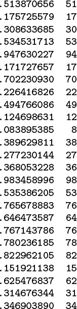
To transform floating-point numbers between 0 and 1 into table indices for a table of size 97, we multiply by 97. In this example, there are three collisions: at 17, 53, and 76. The most significant bits of the keys determine the hash values; the least significant bits of the keys play no role. One goal of hash-function design is to avoid such imbalance by having each bit of data play a role in the computation.
Figure 14.1 Multiplicative hash function for floating-point keys
If the keys are w-bit integers, we can convert them to floating-point numbers and divide by 2w to get floating-point numbers between 0 and 1, then multiply by M as in the previous paragraph. If floating-point operations are expensive and the numbers are not so large as to cause overflow, we can accomplish the same result with integer arithmetic operations: Multiply the key by M, then shift right w bits to divide by 2w (or, if the multiply would overflow, shift then multiply). Such functions are not useful for hashing unless the keys are evenly distributed in the range, because the hash value is determined only by the leading digits of the keys.
A simpler and more efficient method for w-bit integers—one that is perhaps the most commonly used method for hashing—is to choose the table size M to be prime, and, for any integer key k, to compute the remainder when dividing k by M, or h(k) = k mod M. Such a function is called a modular hash function. It is easy to compute (k % M, in C), and is effective in dispersing the key values evenly among the values less than M. Figure 14.2 gives a small example.
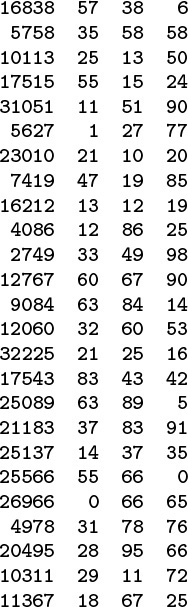
The three rightmost columns show the result of hashing the 16-bit keys on the left with these functions:
v % 97 (left)v % 100 (center) and(int) (a * v) % 100 (right)
where a = .618033. The table sizes for these functions are 97, 100, and 100, respectively. The values appear random (because the keys are random). The center function (v % 100) uses just the rightmost two digits of the keys and is therefore susceptible to bad performance for nonrandom keys.
Figure 14.2 Modular hash functions for integer keys
We can also use modular hashing for floating-point keys. If the keys are in a small range, we can scale to convert them to numbers between 0 and 1, multiply by 2w to get a w-bit integer result, then use a modular hash function. Another alternative is just to use the binary representation of the key (if available) as the operand for the modular hashing function.
Modular hashing applies whenever we have access to the bits that our keys comprise, whether they are integers represented in a machine word, a sequence of characters packed into a machine word, or any of a myriad of other possibilities. A sequence of random characters packed into a machine word is not quite the same as a random integer key, because some of the bits are used for encoding purposes, but we can make both (and any other type of key that is encoded so as to fit in a machine word) appear to be random indices into a small table.
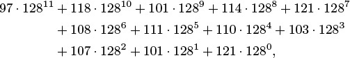
Figure 14.3 illustrates the primary reason that we choose the hash table size M to be prime for modular hashing. In this example, for character data with 7-bit encoding, we treat the key as a base-128 number—one digit for each character in the key. The word now corresponds to the number 1816567, which also can be written as
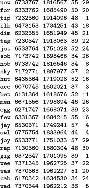
Each line in this table shows a 3-character word, that word’s ASCII encoding as a 21-bit number in octal and decimal, and standard modular hash functions for table sizes 64 and 31, respectively (right-most two columns). The table size 64 leads to undesirable results, because only the rightmost bits of the keys contribute to the hash value, and characters in natural-language words are not evenly distributed. For example, all words ending in y hash to the value 57. By contrast, the prime value 31 leads to fewer collisions in a table less than one-half the size.
Figure 14.3 Modular hash functions for encoded characters
110 · 1282 + 111 · 1281 + 119 · 1280
since the ASCII encodings of n, o, and w are 1568 = 110, 1578 = 111, and 1678 = 119, respectively. Now, the choice of table size M = 64 is unfortunate for this type of key, because the value of x mod 64 is unaffected by the addition of multiples of 64 (or 128) to x—the hash function of any key is the value of that key’s last 6 bits. Surely a good hash function should take into account all the bits of a key, particularly for keys made up of characters. Similar effects can arise whenever M has a factor that is a power of 2. The simplest way to avoid such effects is to make M prime.
Modular hashing is completely trivial to implement except for the requirement that we make the table size prime. For some applications, we can be content with a small known prime, or we can look up a prime number close to the table size that we want in a list of known primes. For example, numbers of the form 2t – 1 are prime for t = 2, 3, 5, 7, 13, 17, 19, and 31 (and no other t < 31): these are the famous Mersenne primes. To allocate a table of a certain size dynamically, we would need to compute a prime number close to a certain value. This calculation is not a trivial one (although there is a clever algorithm for the task, which we shall examine in Part 5), so, in practice, a common solution is to use a precomputed table (see Figure 14.4). Use of modular hashing is not the only reason to make a table size prime; we shall consider another reason in Section 14.4.
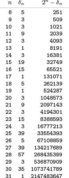
This table of the largest prime less than 2n for 8 ≤ n ≤ 32 can be used to dynamically allocate a hash table, when it is required that the table size be prime. For any given positive value in the range covered, we can use this table to get a prime number within a factor of 2 of that value.
Figure 14.4 Prime numbers for hash tables
Another alternative for integer keys is to combine the multiplicative and modular methods: Multiply the key by a constant between 0 and 1, then reduce it modulo M. That is, use the function h(k) = ![]() kα
kα![]() mod M. There is interplay among the values of α, M, and the effective radix of the key that could possibly result in anomalous behavior, but if we use an arbitrary value of α, we are not likely to encounter trouble in a practical application. A popular choice for α is φ = 0.618033 ... (the golden ratio). Many other variations on this theme have been studied, particularly hash functions that can be implemented with efficient machine instructions such as shifting and masking (see reference section).
mod M. There is interplay among the values of α, M, and the effective radix of the key that could possibly result in anomalous behavior, but if we use an arbitrary value of α, we are not likely to encounter trouble in a practical application. A popular choice for α is φ = 0.618033 ... (the golden ratio). Many other variations on this theme have been studied, particularly hash functions that can be implemented with efficient machine instructions such as shifting and masking (see reference section).
In many applications where symbol tables are used, the keys are not numbers and are not necessarily short, but rather are alphanumeric strings and possibly are long. How do we compute the hash function for a word such as
averylongkey?
In 7-bit ASCII, this word corresponds to the 84-bit number
which is too large to be represented for normal arithmetic functions in most computers. Moreover, we should be able to handle keys that are much longer.
To compute a modular hash function for long keys, we transform the keys piece by piece. We can take advantage of arithmetic properties of the mod function and use Horner’s algorithm (see Section 4.9).
This method is based on yet another way of writing the number corresponding to keys. For our example, we write the following expression:
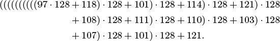
That is, we can compute the decimal number corresponding to the character encoding of a string by proceeding left to right, multiplying the accumulated value by 128, then adding the encoded value of the next character. This computation would eventually produce a number larger than we can represent in our machine for a long string, but we are not interested in computing the number; we want just its remainder when divided by M, which is small. We can get our result without ever carrying a large accumulated value, because we can cast out multiples of M at any point during this computation—we need to keep only the remainder modulo M each time that we do a multiply and add—and we get the same result as we would if we had the capability to compute the long number, then to do the division (see Exercise 14.10). This observation leads to a direct arithmetic way to compute modular hash functions for long strings; see Program 14.1. The program uses one final twist: It uses the prime 127 instead of the base 128. The reason for this change is discussed in the next paragraph.
There are many ways to compute hash functions at approximately the same cost as doing modular hashing using Horner’s method (one or two arithmetic operations for each character in the key). For random keys, the methods hardly differ, but real keys are hardly random. The opportunity to economically make real keys appear to be random leads us to consider randomized algorithms for hashing—we want hash functions that produce random table indices, no matter what the keys are. Randomization is not difficult to arrange, because there is no requirement that we stick to the letter of the definition of modular hashing—we merely want to involve all the bits of the key in a computation that produces an integer less than M. Program 14.1 shows one way to do that: Use a prime base, instead of the power of 2 called for in the definition of the integer corresponding to the ASCII representation of the string. Figure 14.5 illustrates how this change avoids poor dispersion for typical string keys. The hash values produced by Program 14.1 could theoretically be bad for table sizes that are a multiple of 127 (although these effects are likely to be minimal in practice); we could choose the multiplier value at random to produce a randomized algorithm. An even more effective approach is to use random values for the coefficients in the computation, and a different random value for each digit in the key. This approach gives a randomized algorithm called universal hashing.

These diagrams show the dispersion for a set of English words (the first 1000 distinct words of Melville’s Moby Dick) using Program 14.1 with
M = 96 and a = 128 (top)M = 97 and a = 128 (center) andM = 96 and a = 127 (bottom)
Poor dispersion in the first instance results from the combination of uneven usage of the letters and the common factor 32 in the table size and multiplier, which preserves the unevenness. The other two instances appear random because the table size and the multiplier are relatively prime.
Figure 14.5 Hash functions for character strings
A theoretically ideal universal hash function is one for which the chance of a collision between two distinct keys in a table of size M is precisely 1/M. It is possible to prove that using a sequence of different random values, instead of a fixed arbitrary value, for the coefficient a in Program 14.1 turns modular hashing into a universal hash function. We can implement this idea by maintaining an array with a different random number for each key character position. Program 14.2 illustrates an even simpler alternative that performs well in practice—we use a simple pseudorandom sequence for the coefficients.
In summary, to use hashing for an abstract symbol-table implementation, the first step is to extend the abstract type interface to include a hash operation that maps keys into nonnegative integers less than M, the table size. The direct implementation
#define hash(v, M) (((v-s)/(t-s))* M)
does the job for floating-point keys between the values s and t; for integer keys, we can use
#define hash(v, M) (v % M).
If M is not prime,
#define hash(v, M) ((int) (.616161 * (float) v) % M)
or a similar integer computation such as
#define hash(v, M) (16161 * (unsigned) v) % M)
will suffice to spread out the keys. All of these functions, including Program 14.1 for string keys, are venerable ones that have served programmers well for years. The universal method of Program 14.2 is a distinct improvement for string keys that provides random hash values at little extra cost, and we can craft similar randomized methods for integer keys (see Exercise 14.1).
Universal hashing could prove to be much slower than simpler methods in a given application, because doing two arithmetic operations for each character of the key could be overly time-consuming for long keys. To respond to this objection, we can process the key in bigger pieces. Indeed, we may as well use the largest pieces that can fit into a machine word, as in elementary modular hashing. As we discussed in detail previously, an operation of this kind can be difficult or can require special loopholes in some strongly typed high-level languages, but it can be inexpensive or require absolutely no work in C if we use casting among appropriate data-representation formats. These factors are important to consider in many situations because the computation of the hash function might be in the inner loop, so, by speeding up the hash function, we might speed up the whole computation.
Despite the evidence in favor of these methods, care is required in implementing them, for two reasons. First, we have to be vigilant to avoid bugs when converting among types and using arithmetic functions on various different machine representations of keys. Such operations are notorious sources of error, particularly when a program is converted from an old machine to a new one with a different number of bits per word or with other precision differences. Second, the hash-function computation is likely to fall in the inner loop in many applications, and its running time may well dominate the total running time. In such cases, it is important to be sure that it reduces to efficient machine code. Such operations are notorious sources of inefficiency—for example, the difference in running time between the simple modular method and the version where we multiply by 0.61616 first can be startling on a machine with slow hardware or software for floating-point operations. The fastest method of all, for many machines, is to make M a power of 2, and to use the hash function
#define hash(v, M) (v & (M-1)).
This function uses only the least-significant bits of the keys, but the bitwise and operation may be sufficiently faster than integer division to offset any ill effects from poor key dispersion.
A bug that typically arises in hashing implementations is for the hash function always to return the same value, perhaps because an intended type conversion did not take place properly. Such a bug is called a performance bug because a program using such a hash function is likely to run correctly, but to be extremely slow (because it was designed to be efficient only when the hash values are well dispersed). The one-line implementations of these functions are so easy to test that we are well-advised to check how well they perform for the types of keys that are to be encountered for any particular symbol-table implementation.
We can use a χ2 statistic to test the hypothesis that a hash function produces random values (see Exercise 14.5), but this requirement is perhaps too stringent. Indeed, we might be happy if the hash function produces each value the same number of times, which corresponds to a χ2 statistic that is equal to 0, and is decidedly not random. Still, we should be suspicious of huge χ2 statistics. In practice, it probably suffices to use a test that the values are sufficiently well-spread that no value dominates (see Exercise 14.15). In the same spirit, a well-engineered implementation of a symbol-table implementation based on universal hashing might occasionally check that hash values are not poorly dispersed. The client might be informed that either a low-probability event has happened or there is a bug in the hash function. This kind of check would be a wise addition to any practical randomized algorithm.
Exercises
![]() 14.1 Using the
14.1 Using the digit abstraction from Chapter 10 to treat a machine word as a sequence of bytes, implement a randomized hash function for keys represented as bits in machine words.
14.2 Check whether there is any execution-time overhead in converting from a 4-byte key to a 32-bit integer in your programming environment.
![]() 14.3 Develop a hash function for string keys based on the idea of loading 4 bytes at a time, then performing arithmetic operations on 32 bits at a time. Compare the time required for this function with the times for Program 14.1 for 4-, 8-, 16-, and 32-byte keys.
14.3 Develop a hash function for string keys based on the idea of loading 4 bytes at a time, then performing arithmetic operations on 32 bits at a time. Compare the time required for this function with the times for Program 14.1 for 4-, 8-, 16-, and 32-byte keys.
14.4 Write a program to find values of a and M, with M as small as possible, such that the hash function a*x % M produces distinct values (no collisions) for the keys in Figure 14.2. The result is an example of a perfect hash function.
![]() 14.5 Write a program to compute the χ2 statistic for the hash values of N keys with table size M. This number is defined by the equation
14.5 Write a program to compute the χ2 statistic for the hash values of N keys with table size M. This number is defined by the equation
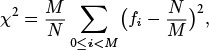
where fi is the number of keys with hash value i. If the hash values are random, this statistic, for N > cM, should be ![]() with probability 1 – 1/c.
with probability 1 – 1/c.
14.6 Use your program from Exercise 14.5 to evaluate the hash function 618033*x % 10000 for keys that are random positive integers less than 106.
14.7 Use your program from Exercise 14.5 to evaluate the hash function in Program 14.1 for distinct string keys taken from some large file on your system, such as a dictionary.
![]() 14.8 Suppose that keys are t-bit integers. For a modular hash function with prime M, prove that each key bit has the property that there exist two keys differing only in that bit with different hash values.
14.8 Suppose that keys are t-bit integers. For a modular hash function with prime M, prove that each key bit has the property that there exist two keys differing only in that bit with different hash values.
14.9 Consider the idea of implementing modular hashing for integer keys with the code (a*x) % M, where a is an arbitrary fixed prime. Does this change mix up the bits sufficiently well that you can use nonprime M?
14.10 Prove that (((ax) mod M) + b) mod M = (ax + b) mod M, assuming that a, b, x, and M are all nonnegative integers.
![]() 14.11 If you use the words from a text file, such as a book, in Exercise 14.7, you are unlikely to get a good χ2 statistic. Explain why this assertion is true.
14.11 If you use the words from a text file, such as a book, in Exercise 14.7, you are unlikely to get a good χ2 statistic. Explain why this assertion is true.
14.12 Use your program from Exercise 14.5 to evaluate the hash function 97*x % M, for all table sizes between 100 and 200, using 103 random positive integers less than 106 as keys.
14.13 Use your program from Exercise 14.5 to evaluate the hash function 97*x % M, for all table sizes between 100 and 200, using the integers between 102 and 103 as keys.
14.14 Use your program from Exercise 14.5 to evaluate the hash function 100*x % M, for all table sizes between 100 and 200, using 103 random positive integers less than 106 as keys.
14.15 Do Exercises 14.12 and 14.14, but use the simpler criterion of rejecting hash functions that produce any value more than 3N/M times.
14.2 Separate Chaining
The hash functions discussed in Section 14.1 convert keys into table addresses; the second component of a hashing algorithm is to decide how to handle the case when two keys hash to the same address. The most straightforward method is to build, for each table address, a linked list of the items whose keys hash to that address. This approach leads directly to the generalization of elementary list search (see Chapter 12) that is given in Program 14.3. Rather than maintaining a single list, we maintain M lists.
This method is traditionally called separate chaining, because items that collide are chained together in separate linked lists. An example is depicted in Figure 14.6. As with elementary sequential search, we can choose to keep the lists in sorted order, or we can leave them unordered. The same basic tradeoffs as those discussed in Section 12.3 apply, but, for separate chaining, the time savings are less significant (because the lists are short) and the space usage is more significant (because there are so many lists).
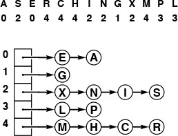
This diagram shows the result of inserting the keys A S E R C H I N G X M P L into an initially empty hash table with separate chaining (unordered lists), using the hash values given at the top. The A goes into list 0, then the S goes into list 2, then the E goes into list 0 (at the front, to keep the insertion time constant), then the R goes into list 4, and so forth.
Figure 14.6 Hashing with separate chaining
We might be using a header node to streamline the code for insertion into an ordered list, but we might not want to use M header nodes for individual lists in separate chaining. Indeed, we could even eliminate the M links to the lists by having the first nodes in the lists comprise the table (see Exercise 14.20).
For a search miss, we can assume that the hash function scrambles the key values sufficiently well that each of the M lists is equally likely to be searched. Then the performance characteristics that we studied in Section 12.3 apply, for each list.
Property 14.1 Separate chaining reduces the number of comparisons for sequential search by a factor of M (on the average), using extra space for M links.
The average length of the lists is N/M. As described in Chapter 12, successful searches are expected to go about halfway down some list. Unsuccessful searches go to the end of a list if the lists are unordered, halfway down a list if the lists are kept in order. ![]()
Most often, we use unordered lists for separate chaining, because that approach is both easy to implement and efficient: insert takes constant time and search takes time proportional to N/M. If huge numbers of search misses are expected, we can speed up the misses by a factor of 2 by keeping the lists ordered, at the cost of a slower insert.
As stated, Property 14.1 is a trivial result, because the average length of the lists is N/M, no matter how the items are distributed among the lists. For example, suppose that all the items fall onto the first list. Then, the average length of the lists is (N +0+0+...+0)/M = N/M. The real reason that hashing is useful in practice is that each list is extremely likely to have about N/M items.
Property 14.2 In a separate-chaining hash table with M lists and N keys, the probability that the number of keys in each list is within a small constant factor of N/M is extremely close to 1.
We briefly consider this classical analysis, for readers who are familiar with basic probabilistic analysis. The probability that a given list will have k items on it is
by an elementary argument. We choose k out of the N items: Those k items hash to the given list with probability 1/M, and the other N – k items do not hash to the given list with probability 1 – (1/M). In terms of α = N/M, we can rewrite this expression as
which, by the classical Poisson approximation, is less than
From this result, it follows that the probability that a list has more than tα items on it is less than
This probability is extremely small for practical ranges of the parameters. For example, if the average length of the lists is 20, the probability that we will hash to some list with more than 40 items on it is less than (20e/2)2e–20 ≈ 0.0000016. ![]()
The foregoing analysis is an example of a classical occupancy problem, where we consider N balls thrown randomly into one of M urns, and analyze how the balls are distributed among the urns. Classical mathematical analysis of these problems tells us many other interesting facts that are relevant to the study of hashing algorithms. For example, the Poisson approximation tells us that the number of empty lists is about e–α. A more interesting result tells us that the average number of items inserted before the first collision occurs is about ![]() . This result is the solution to the classical birthday problem. For example, the same analysis tells us, for M = 365, that the average number of people we need to check before finding two with the same birthday is about 24. A second classical result tells us that the average number of items inserted before each list has at least one item is about M HM. This result is the solution to the classical coupon collector problem. For example, the same analysis tells us, for M = 1280, that we would expect to collect 9898 baseball cards (coupons) before getting one for each of 40 players on each of 32 teams in a series.
. This result is the solution to the classical birthday problem. For example, the same analysis tells us, for M = 365, that the average number of people we need to check before finding two with the same birthday is about 24. A second classical result tells us that the average number of items inserted before each list has at least one item is about M HM. This result is the solution to the classical coupon collector problem. For example, the same analysis tells us, for M = 1280, that we would expect to collect 9898 baseball cards (coupons) before getting one for each of 40 players on each of 32 teams in a series.
These research results are indicative of the properties of hashing that have been analyzed. In practice, they tell us that we can use separate chaining with great confidence, if the hash function produces values that approximate random ones (see reference section).
In a separate-chaining implementation, we typically choose M to be small enough that we are not wasting a huge area of contiguous memory with empty links, but large enough that sequential search is the most efficient method for the lists. Hybrid methods (such as using binary trees instead of linked lists) are probably not worth the trouble. As a rule of thumb, we might choose M to be about one-fifth or one-tenth the number of keys expected be be in the table, so that the lists are expected to contain about five or 10 keys each. One of the virtues of separate chaining is that this decision is not critical: if more keys arrive than expected, then searches will take a little longer than if we had chosen a bigger table size ahead of time; if fewer keys are in the table, then we have extra-fast search with perhaps a small amount of wasted space. When space is not a critical resource, M can be chosen sufficiently large that search time is constant; when space is a critical resource, we still can get a factor of M improvement in performance by choosing M to be as large as we can afford.
The comments in the previous paragraph apply to search time. In practice, unordered lists are normally used for separate chaining, for two primary reasons. First, as we have mentioned, insert is extremely fast: We compute the hash function, allocate memory for the node, and link in the node at the beginning of the appropriate list. In many applications, the memory-allocation step is not needed (because the items inserted into the symbol table may be existing records with available link fields), and we are left with perhaps three or four machine instructions for insert. The second important advantage of using the unordered-list implementation in Program 14.3 is that the lists all function as stacks, so we can easily remove the most recently inserted items, which are at the front of the lists (see Exercise 14.21). This operation is an important one when we are implementing a symbol table with nested scopes, for example in a compiler.
As in several previous implementations, we implicitly give the client a choice for handling duplicate keys. A client like Program 12.10 might search to check for duplicates before any insert, thus ensuring that the table does not contain any duplicate keys. Another client might avoid the cost of this search by leaving duplicates in the table, thus achieving fast insert operations.
Generally, hashing is not appropriate for use in applications where implementations for the sort and select ADT operations are required. However, hashing is often used for the typical situation where we need to use a symbol table with potentially a large number of search, insert, and delete operations, then to print out the items in order of their keys once, at the end. One example of such an application is a symbol table in a compiler; another is a program to remove duplicates, such as Program 12.10. To handle this situation in an unordered-list implementation of separate chaining, we would have to use one of the sorting methods described in Chapters 6 through 10;in an ordered-list implementation, we could accomplish the sort in time proportional to N lg M with list mergesort (see Exercise 14.23).
Exercises
![]() 14.16 How long could it take in the worst case to insert N keys into an initially empty table, using separate chaining with (i) unordered lists and (ii) ordered lists?
14.16 How long could it take in the worst case to insert N keys into an initially empty table, using separate chaining with (i) unordered lists and (ii) ordered lists?
![]() 14.17 Give the contents of the hash table that results when you insert items with the keys E A S Y Q U T I O N in that order into an initially empty table of M = 5 lists, using separate chaining with unordered lists. Use the hash function 11k mod M to transform the kth letter of the alphabet into a table index.
14.17 Give the contents of the hash table that results when you insert items with the keys E A S Y Q U T I O N in that order into an initially empty table of M = 5 lists, using separate chaining with unordered lists. Use the hash function 11k mod M to transform the kth letter of the alphabet into a table index.
![]() 14.18 Answer Exercise 14.17, but use ordered lists. Does your answer depend on the order in which you insert the items?
14.18 Answer Exercise 14.17, but use ordered lists. Does your answer depend on the order in which you insert the items?
![]() 14.19 Write a program that inserts N random integers into a table of size N/100 using separate chaining, then finds the length of the shortest and longest lists, for N = 103, 104, 105, and 106.
14.19 Write a program that inserts N random integers into a table of size N/100 using separate chaining, then finds the length of the shortest and longest lists, for N = 103, 104, 105, and 106.
14.20 Modify Program 14.3 to eliminate the head links by representing the symbol table as an array of STnodes (each table entry is the first node in its list).
14.21 Modify Program 14.3 to include an integer field for each item that is set to the number of items in the table at the time the item is inserted. Then implement a function that deletes all items for which the field is greater than a given integer N.
14.22 Modify the implementation of STsearch in Program 14.3 to visit all the items with keys equal to a given key, in the same manner as STsort.
14.23 Implement a symbol table using separate chaining with ordered lists (with a fixed table of size 97) that supports the initialize, count, search, insert, delete, join, select, and sort operations for a first-class symbol-table ADT, with support for client handles (see Exercises 12.4 and 12.5).
14.3 Linear Probing
If we can estimate in advance the number of elements to be put into the hash table and have enough contiguous memory available to hold all the keys with some room to spare, then it is probably not worthwhile to use any links at all in the hash table. Several methods have been devised that store N items in a table of size M > N, relying on empty places in the table to help with collision resolution. Such methods are called open-addressing hashing methods.
The simplest open-addressing method is called linear probing: when there is a collision (when we hash to a place in the table that is already occupied with an item whose key is not the same as the search key), then we just check the next position in the table. It is customary to refer to such a check (determining whether or not a given table position holds an item with key equal to the search key) as a probe. Linear probing is characterized by identifying three possible outcomes of a probe: if the table position contains an item whose key matches the search key, then we have a search hit; if the table position is empty, then we have a search miss; otherwise (if the table position contains an item whose key does not match the search key) we just probe the table position with the next higher index, continuing (wrapping back to the beginning of the table if we reach the end) until either the search key or an empty table position is found. If an item containing the search key is to be inserted following an unsuccessful search, then we put it into the empty table space that terminated the search. Program 14.4 is an implementation of the symbol-table ADT using this method. The process of constructing a hash table for a sample set of keys using linear probing is shown in Figure 14.7.
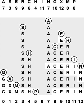
This diagram shows the process of inserting the keys A S E R C H I N G X M P into an initially empty hash table of size 13 with open addressing, using the hash values given at the top and resolving collisions with linear probing. First, the A goes into position 7, then the S goes into position 3, then the E goes into position 9, then the R goes into position 10 after a collision at position 9, and so forth. Probe sequences that run off the right end of the table continue on the left end: for example, the final key inserted, the P, hashes to position 8, then ends up in position 5 after collisions at positions 8 through 12, then 0 throuh 5. All table positions not probed are shaded.
Figure 14.7 Hashing with linear probing
As with separate chaining, the performance of open-addressing methods is dependent on the ratio α = N/M, but we interpret it differently. For separate chaining, α is the average number of items per list and is generally larger than 1. For open addressing, α is the fraction of those table positions that are occupied; it must be less than 1. We sometimes refer to α as the load factor of the hash table.
For a sparse table (small α), we expect most searches to find an empty position with just a few probes. For a nearly full table (α close to 1), a search could require a huge number of probes, and could even fall into an infinite loop when the table is completely full. Typically, we insist that the table not be allowed to become nearly full when using linear probing, to avoid long search times. That is, rather than using extra memory for links, we use it for extra space in the hash table that shortens probe sequences. The table size for linear probing is greater than for separate chaining, since we must have M > N, but the total amount of memory space used may be less, since no links are used. We will discuss space-usage comparisons in detail in Section 14.5; for the moment, we consider the analysis of the running time of linear probing as a function of α.
The average cost of linear probing depends on the way in which the items cluster together into contiguous groups of occupied table cells, called clusters, when they are inserted. Consider the following two extremes in a linear probing table that is half full (M = 2N): In the best case, table positions with even indices could be empty, and table positions with odd indices could be occupied. In the worst case, the first half of the table positions could be empty, and the second half occupied. The average length of the clusters in both cases is N/(2N) = 1/2, but the average number of probes for an unsuccessful search is 1 (all searches take at least 1 probe) plus
(0 + 1 + 0 + 1 + ...)/(2N) = 1/2
in the best case, and is 1 plus
(N + (N – 1) + (N – 2) + ...)/(2N) ≈ N/4
in the worst case.
Generalizing this argument, we find that the average number of probes for an unsuccessful search is proportional to the squares of the lengths of the clusters. We compute the average by computing the cost of a search miss starting at each position in the table, then dividing the total by M. All search misses take at least 1 probe, so we count the number of probes after the first. If a cluster is of length t, then the expression
(t + (t – 1) + ... + 2 + 1)/M = t(t + 1)/(2M)
counts the contribution of that cluster to the grand total. The sum of the cluster lengths is N, so, adding this cost for all cells in the table, we find that the total average cost for a search miss is 1+ N/(2M) plus the sum of the squares of the lengths of the clusters, divided by 2M. Given a table, we can quickly compute the average cost of unsuccessful search in that table (see Exercise 14.28), but the clusters are formed by a complicated dynamic process (the linear-probing algorithm) that is difficult to characterize analytically.
Property 14.3 When collisions are resolved with linear probing, the average number of probes required to search in a hash table of size M that contains N = αM keys is about
for hits and misses, respectively.
Despite the relatively simple form of the results, precise analysis of linear probing is a challenging task. Knuth’s completion of it in 1962 was a landmark in the analysis of algorithms (see reference section). ![]()
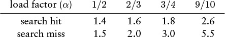
These estimates lose accuracy as α approaches 1, but we do not need them for that case, because we should not be using linear probing in a nearly full table in any event. For smaller α, the equations are sufficiently accurate. The following table summarizes the expected number of probes for search hits and misses with linear probing:
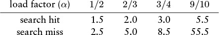
Search misses are always more expensive than hits, and both require only a few probes, on the average, in a table that is less than half full.
As we did with separate chaining, we leave to the client the choice of whether or not to keep items with duplicate keys in the table. Such items do not necessarily appear in contiguous positions in a linear probing table—other items with the same hash value can appear among items with duplicate keys.
By the very nature of the way the table is constructed, the keys in a table built with linear probing are in random order. The sort and select ADT operations require starting from scratch with one of the methods described in Chapters 6 through 10, so linear probing is not appropriate for applications where these operations are performed frequently.
How do we delete a key from a table built with linear probing? We cannot just remove it, because items that were inserted later might have skipped over that item, so searches for those items would terminate prematurely at the hole left by the deleted item. One solution to this problem is to rehash all the items for which this problem could arise—those between the deleted one and the next unoccupied position to the right. Figure 14.8 shows an example illustrating this process; Program 14.5 is an implementation. In a sparse table, this repair process will require only a few rehash operations, at most. Another way to implement deletion is to replace the deleted key with a sentinel key that can serve as a placeholder for searches but can be identified and reused for insertions (see Exercise 14.33).
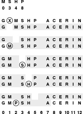
This diagram shows the process of deleting the X from the table in Figure 14.7. The second line shows the result of just taking the X out of the table, and is an unacceptable final result because the M and the P are cut off from their hash positions by the empty table position left by the X. Thus, we reinsert the M, S, H, and P (the keys to the right of the X in the same cluster), in that order, using the hash values given at the top and resolving collisions with linear probing. The M fills the hole left by the X, then the S and the H hash into the table without collisions, then the P winds up in position 2.
Figure 14.8 Deletion in a linear-probing hash table
Exercises
![]() 14.24 How long could it take, in the worst case, to insert N keys into an initially empty table, using linear probing?
14.24 How long could it take, in the worst case, to insert N keys into an initially empty table, using linear probing?
![]() 14.25 Give the contents of the hash table that results when you insert items with the keys E A S Y Q U T I O N in that order into an initially empty table of size M = 16 using linear probing. Use the hash function 11k mod M to transform the kth letter of the alphabet into a table index.
14.25 Give the contents of the hash table that results when you insert items with the keys E A S Y Q U T I O N in that order into an initially empty table of size M = 16 using linear probing. Use the hash function 11k mod M to transform the kth letter of the alphabet into a table index.
14.26 Do Exercise 14.25 for M = 10.
![]() 14.27 Write a program that inserts 105 random nonnegative integers less than 106 into a table of size 105 using linear probing, and that plots the total number of probes used for each 103 consecutive insertions.
14.27 Write a program that inserts 105 random nonnegative integers less than 106 into a table of size 105 using linear probing, and that plots the total number of probes used for each 103 consecutive insertions.
14.28 Write a program that inserts N/2 random integers into a table of size N using linear probing, then computes the average cost of a search miss in the resulting table from the cluster lengths, for N = 103, 104, 105, and 106.
14.29 Write a program that inserts N/2 random integers into a table of size N using linear probing, then computes the average cost of a search hit in the resulting table, for N = 103, 104, 105, and 106. Do not search for all the keys at the end (keep track of the cost of constructing the table).
![]() 14.30 Run experiments to determine whether the average cost of search hits or search misses changes as a long sequence of alternating random insertions and deletions using Programs 14.4 and 14.5 is made in a hash table of size 2N with N keys, for N = 10, 100, and 1000, and for up to N2 insertion–deletion pairs for each N.
14.30 Run experiments to determine whether the average cost of search hits or search misses changes as a long sequence of alternating random insertions and deletions using Programs 14.4 and 14.5 is made in a hash table of size 2N with N keys, for N = 10, 100, and 1000, and for up to N2 insertion–deletion pairs for each N.
14.4 Double Hashing
The operative principle of linear probing (and indeed of any hashing method) is a guarantee that, when we are searching for a particular key, we look at every key that hashes to the same table address (in particular, the key itself, if it is in the table). In an open addressing scheme, however, other keys are typically also examined, particularly when the table begins to fill up. In the example depicted in Figure 14.7, a search for N involves looking at C, E. R, and I, none of which had the same hash value. What is worse, insertion of a key with one hash value can drastically increase the search times for keys with other hash values: in Figure 14.7, the insertion of M caused increased search times for positions 7–12 and 0–1. This phenomenon is called clustering because it has to do with the process of cluster formation. It can make linear probing run slowly for nearly full tables.
Fortunately, there is an easy way to virtually eliminate the clustering problem: double hashing. The basic strategy is the same as for linear probing; the only difference is that, instead of examining each successive table position following a collision, we use a second hash function to get a fixed increment to use for the probe sequence. An implementation is given in Program 14.6.
The second hash function must be chosen with some care, since otherwise the program may not work at all. First, we must exclude the case where the second hash function evaluates to 0, since that would lead to an infinite loop on the very first collision. Second, it is important that the value of the second hash function be relatively prime to the table size, since otherwise some of the probe sequences could be very short (for example, consider the case where the table size is twice the value of the second hash function). One way to enforce this policy is to make M prime and to choose a second hash function that returns values that are less than M. In practice, a simple second hash function such as
#define hashtwo(v) ((v % 97)+1)
will suffice for many hash functions, when the table size is not small. Also in practice, any loss in efficiency that is due to this simplification is not likely to be noticeable, much less to be significant. If the table is huge and sparse, the table size itself does not need to be prime because just a few probes will be used for every search (although we might want to test for and abort long searches to guard against an infinite loop, if we cut this corner (see Exercise 14.38)).
Figure 14.9 shows the process of building a small table with double hashing; Figure 14.10 shows that double hashing results in many fewer clusters (which are therefore much shorter) than the clusters left by linear probing.

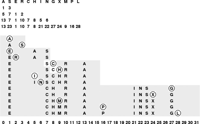
This diagram shows the process of inserting the keys A S E R C H I N G X M P L into an initially empty hash table with open addressing, using the hash values given at the top and resolving collisions with double hashing. The first and second hash values for each key appear in the two rows below that key. As in Figure 14.7, table positions that are probed are unshaded. The A goes into position 7, then the S goes into position 3, then the E goes into position 9, as in Figure 14.7, but the R goes into position 1 after the collision at position 9, using its second hash value of 5 for the probe increment after collision. Similarly, P goes into position 6 on the final insertion after collisions at positions 8, 12, 3, 7, 11, and 2, using its second hash value 4 as the probe increment.
Figure 14.9 Double hashing

These diagrams show the placement of records as we insert them into a hash table using linear probing (center) and double hashing (bottom), with the key value distribution shown at the top. Each line shows the result of inserting 10 records. As the table fills, the records cluster together into sequences separated by empty table positions. Long clusters are undesirable because the average cost of searching for one of the keys in the cluster is proportional to the cluster length. With linear probing, the longer clusters are, the more likely they are to increase in length, so a few long clusters dominate as the table fills up. With double hashing, this effect is much less pronounced, and the clusters remain relatively short.
Figure 14.10 Clustering
Property 14.4 When collisions are resolved with double hashing, the average number of probes required to search in a hash table of size M that contains N = αM keys is
for hits and misses, respectively.
These formulas are the result of a deep mathematical analysis done by Guibas and Szemeredi (see reference section). The proof is based on showing that double hashing is nearly equivalent to a more complicated random hashing algorithm where we use a key-dependent sequence of probe positions with each probe equally likely to hit each table position. This algorithm is only an approximation to double hashing for many reasons: for example, we take pains in double hashing to ensure that we try every table position once, but random hashing could examine the same table position more than once. Still, for sparse tables, the probabilities of collisions for the two methods are similar. We are interested in both: Double hashing is easy to implement, whereas random hashing is easy to analyze.
The average cost of a search miss for random hashing is given by the equation
The expression on the left is the sum of the probability that a search miss uses more than k probes, for k = 0, 1, 2,... (and is equal to the average from elementary probability theory). A search always uses one probe, then needs a second probe with probability N/M, a third probe with probability (N/M)2, and so forth. We can also use this formula to compute the following approximation to the average cost of a search hit in a table with N keys:
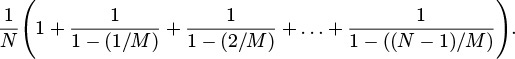
Each key in the table is equally likely to be hit; the cost of finding a key is the same as the cost of inserting it; and the cost of inserting the jth key in the table is the cost of a search miss in a table of j – 1 keys, so this formula is the average of those costs. Now, we can simplify and evaluate this sum by multiplying the top and bottom of all the fractions by M:
and further simplify to get the result
since HM ≈ ln M. ![]()
The precise nature of the relationship between the performance of double hashing and the random-hashing ideal that was proven by Guibas and Szemeredi is an asymptotic result that need not be relevant for practical table sizes; moreover, the results rest on the assumption that the hash functions return random values. Still, the asymptotic formulas in Property 14.5 are accurate predictors of the performance of double hashing in practice, even when we use an easy-to-compute second hash function such as (v % 97)+1. As do the corresponding formulas for linear probing, these formulas approach infinity as α approaches 1, but they do so much more slowly.
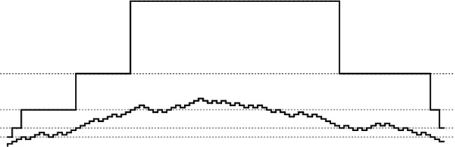
The contrast between linear probing and double hashing is illustrated clearly in Figure 14.11. Double hashing and linear probing have similar performance for sparse tables, but we can allow the table to become more nearly full with double hashing than we can with linear probing before performance degrades. The following table summarizes the expected number of probes for search hits and misses with double hashing:
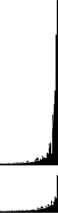
These plots show the costs of building a hash table of size 1000 by inserting keys into an initially empty table using linear probing (top) and double hashing (bottom). Each bar represents the cost of 20 keys. The gray curves show the costs predicted by theoretical analysis (see Properties 14.4 and 14.5).
Figure 14.11 Costs of open-addressing search
Search misses are always more expensive than hits, and both require only a few probes, on the average, even in a table that is nine-tenths full.
Looking at the same results in another way, double hashing allows us to use a smaller table than we would need with linear probing to get the same average search times.
Property 14.5 We can ensure that the average cost of all searches is less than t probes by keeping the load factor less than ![]() for linear probing and less than 1 – 1/t for double hashing.
for linear probing and less than 1 – 1/t for double hashing.
Set the equations for search misses in Property 14.4 and Property 14.5 equal to t, and solve for α. ![]()
For example, to ensure that the average number of probes for a search is less than 10, we need to keep the table at least 32 percent empty for linear probing, but only 10 percent empty for double hashing. If we have 105 items to process, we need space for just another 104 items to be able to do unsuccessful searches with fewer than 10 probes. By contrast, separate chaining would require more than 105 links, and BSTs would require twice that many.
The method of Program 14.5 for implementing the delete operation (rehash the keys that might have a search path containing the item to be deleted) breaks down for double hashing, because the deleted key might be in many different probe sequences, involving keys throughout the table. Thus, we have to resort to the other method that we considered at the end of Section 12.3: We replace the deleted item with a sentinel that marks the table position as occupied but does not match any key (see Exercise 14.33).
Like linear probing, double hashing is not an appropriate basis for implementing a full-function symbol table ADT where we need to support the sort or select operations.
Exercises
![]() 14.31 Give the contents of the hash table that results when you insert items with the keys E A S Y Q U T I O N in that order into an initially empty table of size M = 16 using double hashing. Use the hash function 11k mod M for the initial probe and the second hash function (k mod 3) + 1 for the search increment (when the key is the kth letter of the alphabet).
14.31 Give the contents of the hash table that results when you insert items with the keys E A S Y Q U T I O N in that order into an initially empty table of size M = 16 using double hashing. Use the hash function 11k mod M for the initial probe and the second hash function (k mod 3) + 1 for the search increment (when the key is the kth letter of the alphabet).
![]() 14.32 Answer Exercise 14.31 for M = 10
14.32 Answer Exercise 14.31 for M = 10
14.33 Implement deletion for double hashing, using a sentinel item.
14.34 Modify your solution to Exercise 14.27 to use double hashing.
14.35 Modify your solution to Exercise 14.28 to use double hashing.
14.36 Modify your solution to Exercise 14.29 to use double hashing.
![]() 14.37 Implement an algorithm that approximates random hashing, by providing the key as a seed to an in-line random number generator (as in Program 14.2).
14.37 Implement an algorithm that approximates random hashing, by providing the key as a seed to an in-line random number generator (as in Program 14.2).
14.38 Suppose that a table of size 106 is half full, with occupied positions chosen at random. Estimate the probability that all positions with indices divisible by 100 are occupied.
![]() 14.39 Suppose that you have a bug in your double-hashing code such that one or both of the hash functions always return the same value (not 0). Describe what happens in each of these situations: (i) when the first one is wrong (ii) when the second one is wrong, and (iii) when both are wrong.
14.39 Suppose that you have a bug in your double-hashing code such that one or both of the hash functions always return the same value (not 0). Describe what happens in each of these situations: (i) when the first one is wrong (ii) when the second one is wrong, and (iii) when both are wrong.
14.5 Dynamic Hash Tables
As the number of keys in a hash table increases, search performance degrades. With separate chaining, the search time increases gradually—when the number of keys in the table doubles, the search time doubles. The same is true of open-addressing methods such as linear probing and double hashing for sparse tables, but the cost increases dramatically as the table fills up, and, worse, we reach a point where no more keys can be inserted at all. This situation is in contrast to search trees, which accommodate growth naturally. For example, in a red–black tree, the search cost increases only slightly (by one comparison) whenever the number of nodes in the tree doubles.
One way to accomplish growth in a hash table is to double the table’s size when it begins to fill up. Doubling the table is an expensive operation because everything in the table has to be reinserted, but it is an operation that is performed infrequently. Program 14.7 is an implementation of growth by doubling for linear probing. An example is depicted in Figure 14.12. The same solution also works for double hashing, and the basic idea applies to separate chaining as well (see Exercise 14.46). Each time that the table gets more than half full, we expand the table by doubling it in size. After the first expansion, the table is always between one-quarter and one-half full, so the search cost is less than three probes, on the average. Furthermore, although the operation of rebuilding the table is expensive, it happens so infrequently that its cost represents only a constant fraction of the total cost of building the table.
This diagram shows the process of inserting the keys A S E R C H I N G X M P L into a dynamic hash table that expands by doubling, using the hash values given at the top and resolving collisions with linear probing. The four rows beneath the keys give the hash values when the table size is 4, 8, 16, and 32. The table size starts at 4, doubles to 8 for the E, to 16 for the C and to 32 for the G. All keys are rehashed and reinserted when the table size doubles. All insertions are into sparse tables (less than one-quarter full for reinsertion, between one-quarter and one-half full otherwise), so there are few collisions.
Figure 14.12 Dynamic hash-table expansion
Another way to express this concept is to say that the average cost per insertion is less than four probes. This assertion is not the same as saying that each insertion requires less than four probes on the average; indeed, we know that those insertions that cause the table to double will require a large number of probes. This argument is a simple example of amortized analysis: We cannot guarantee that each and every operation will be fast for this algorithm, but we can guarantee that the average cost per operation will be low.
Although the total cost is low, the performance profile for insertions is erratic: Most operations are extremely fast, but certain rare operations require about as much time as the whole previous cost of building the table. As a table grows from 1 thousand to 1 million keys, this slowdown will happen about 10 times. This kind of behavior is acceptable in many applications, but it might not be appropriate when absolute performance guarantees are desirable or required. For example, while a bank or an airline might be willing to suffer the consequences of keeping a customer waiting for so long on 10 out of every 1 million transactions, long waits might be catastrophic in other applications, such as an online system implementing a large financial transaction-processing system or in an air-traffic control system.
If we support the delete ADT operation, then it may be worthwhile to contract the table by halving it as it shrinks (see Exercise 14.44), with one proviso: The thresholds for shrinking have to be separated from those for growing, because otherwise a small number of insert and delete operations could cause a sequence of doubling and halving operations even for huge tables.
Property 14.6 A sequence of t search, insert, and delete symbol-table operations can be executed in time proportional to t and with memory usage always within a constant factor of the number of keys in the table.
We use linear probing with growth by doubling whenever an insert causes the number of keys in the table to be half the table size, and we use shrinkage by halving whenever a delete causes the number of keys in the table to be one-eighth the table size. In both cases, after the table is rebuilt to size N, it has N/4 keys. Then, N/4 insert operations must be executed before the table doubles again (by reinsertion of N/2 keys into a table of size 2N), and N/8 delete operations must be executed before the table halves again (by reinsertion of N/8 keys into a table of size N/2). In both cases, the number of keys reinserted is within a factor of 2 of the number of operations that we performed to bring the table to the point of being rebuilt, so the total cost is linear. Furthermore, the table is always between one-eighth and one-fourth full (see Figure 14.13), so the average number of probes for each operation is less than 3, by Property 14.4. ![]()
This diagram shows the number of keys in the table (bottom) and the table size (top) when we insert keys into and delete them from a dynamic hash table using an algorithm that doubles the table when an insert makes it half full and halves the table when a deletion makes it one-eighth full. The table size is initialized at 4 and is always a power of 2 (dotted lines in the figure are at powers of 2). The table size changes when the curve tracing the number of keys in the table crosses a dotted line for the first time after having crossed a different dotted line. The table is always between one-eighth and one-half full.
Figure 14.13 Dynamic hashing
This method is appropriate for use in a symbol-table implementation for a general library where usage patterns are unpredictable, because it can handle tables of all sizes in a reasonable way. The primary drawback is the cost of rehashing and allocating memory when the table expands and shrinks; in the typical case, when searches predominate, the guarantee that the table is sparse leads to excellent performance. In Chapter 16, we shall consider another approach that avoids rehashing and is suitable for huge external search tables.
Exercises
![]() 14.40 Give the contents of the hash table that results when you insert items with the keys E A S Y Q U T I O N in that order into an initially empty table of initial size M = 4 that is expanded with doubling whenever half full, with collisions resolved using linear probing. Use the hash function 11k mod M to transform the kth letter of the alphabet into a table index.
14.40 Give the contents of the hash table that results when you insert items with the keys E A S Y Q U T I O N in that order into an initially empty table of initial size M = 4 that is expanded with doubling whenever half full, with collisions resolved using linear probing. Use the hash function 11k mod M to transform the kth letter of the alphabet into a table index.
14.41 Would it be more economical to expand a hash table by tripling (rather than doubling) the table in size when the table is half full?
14.42 Would it be more economical to expand a hash table by tripling the table in size when the table is one-third full (rather than doubling the table in size when the table is half full)?
14.43 Would it be more economical to expand a hash table by doubling the table in size when the table is three-quarters (rather than half) full?
14.44 Add to Program 14.7 a delete function that deletes an item as in Program 14.4 but then contracts the table by halving it if the deletion leaves it seven-eighths empty.
![]() 14.45 Implement a version of Program 14.7 for separate chaining that increases the table size by a factor of 10 each time the average list length is equal to 10.
14.45 Implement a version of Program 14.7 for separate chaining that increases the table size by a factor of 10 each time the average list length is equal to 10.
14.46 Modify Program 14.7 and your implementation from Exercise 14.44 to use double hashing with lazy deletion (see Exercise 14.33). Make sure that your program takes into account the number of dummy items, as well as the number of empty positions, in making the decisions whether to expand or contract the table.
14.6 Perspective
The choice of the hashing method that is best suited for a particular application depends on many different factors, as we have discussed when examining the methods. All the methods can reduce the symbol-table search and insert functions to constant-time operations, and all are useful for a broad variety of applications. Roughly, we can characterize the three major methods (linear probing, double hashing, and separate chaining) as follows: Linear probing is the fastest of the three (if sufficient memory is available to ensure that the table is sparse), double hashing makes the most efficient use of memory (but requires extra time, to compute the second hash function), and separate chaining is the easiest to implement and deploy (provided that a good storage allocator is available). Table 14.1 gives empirical data and commentary on the performance of the algorithms.
These relative timings for building and searching symbol tables from random sequences of 32-bit integers confirm that hashing is significantly faster than tree search for keys that are easily hashed. Among the hashing methods, double hashing is slower than separate chaining and linear probing for sparse tables (because of the cost of computing the second hash function) but is much faster than linear probing as the table fills, and is the only one of the methods that can provide fast search using only a small amount of extra memory. Dynamic hash tables built with linear probing and expansion by doubling are more costly to construct than are other hash tables because of memory allocation and rehashing, but certainly lead to the fastest search times, and represent the method of choice when search predominates and when the number of keys cannot be predicted accurately in advance.
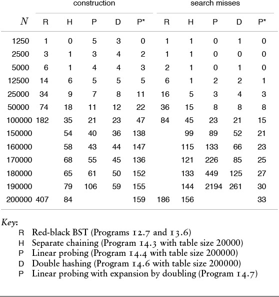
Table 14.1 Empirical study of hash-table implementations
The choice between linear probing and double hashing depends primarily on the cost of computing the hash function and on the load factor of the table. For sparse tables (small α), both methods use only a few probes, but double hashing could take more time because it has to compute two hash functions for long keys. As α approaches 1, double hashing far outperforms linear probing, as we saw in Figure 14.11.
Comparing linear probing and double hashing against separate chaining is more complicated, because we have to account precisely for memory usage. Separate chaining uses extra memory for links; the open-addressing methods use extra memory implicitly within the table to terminate probe sequences. The following concrete example illustrates the situation: Suppose that we have a table of M lists built with separate chaining, that the average length of the lists is 4, and that items and links each occupy a single machine word. The assumption that items and links take the same amount of space is justified in many situations because we would replace huge items with links to the items. With these assumptions, the table uses 9M words of memory (4M for items and 5M for links), and delivers an average search time of 2 probes. But linear probing for 4M items in a table of size 9M requires just (1 + 1/(1 – 4/9))/2 = 1.4 probes for a search hit, a value that is 30 percent faster than separate chaining for the same amount of space; and linear probing for 4M items in a table of size 6M requires 2 probes for a search hit (on the average), and thus uses 33 percent less space than separate chaining for the same amount of time. Furthermore, we can use a dynamic method such as Program 14.7 to ensure that the table can grow while staying sparsely populated.
The argument in the previous paragraph indicates that it is not normally justifiable to choose separate chaining over open addressing on the basis of performance. However, separate chaining with a fixed M is often chosen in practice for a host of other reasons: it is easy to implement (particularly delete); it requires little extra memory for items that have preallocated link fields for use by symbol-table and other ADTs that may need them; and, although its performance degrades as the number of items in the table grows, the degradation is graceful, and takes place in a manner that is unlikely to harm the application because it still is a factor of M faster than sequential search.
Many other hashing methods have been developed that have application in special situations. Although we cannot go into details, we consider three examples briefly to illustrate the nature of specially adapted hashing methods.
One class of methods moves items around during insertion in double hashing to make successful search more efficient. In fact, Brent developed a method for which the average time for a successful search can be bounded by a constant, even in a full table (see reference section). Such a method might be useful in applications where search hits are the predominant operation.
Another method, called ordered hashing, exploits ordering to reduce the cost for unsuccessful search in linear probing to be close to the cost for successful search. In standard linear probing, we stop the search when we find an empty table position or an item with a key equal to the search key; in ordered hashing, we stop the search when we find an item with a key greater than or equal to the search key (the table must be constructed cleverly if this procedure is to work) (see reference section). This improvement by introducing ordering in the table is on the same order as that we achieved by ordering the lists in separate chaining. This method is designed for applications where search misses predominate.
A symbol table that has a fast search miss and somewhat slower search hit can be used to implement an exception dictionary. For example, a text-processing system might have an algorithm for hyphenating words that works well for most words, but does not work for bizarre cases (such as “bizarre”). Only a few words in a huge document are likely to be in the exception dictionary, so nearly all the searches are likely to be misses.
These examples are only a few of a large number of algorithmic improvements that have been suggested for hashing. Many of these improvements are interesting and have important applications. Our usual cautions must be raised against premature use of advanced methods except when the requirements are serious and the performance/complexity tradeoffs are carefully considered, because separate chaining, linear probing and double hashing are simple, efficient, and acceptable for most applications.
The problem of implementing an exception dictionary is an example of an application where we can recast our algorithm slightly to optimize performance for the most frequently performed operation—in this case search miss. For example, suppose that we have a 1000-item exception dictionary, have 1 million items to look up in the dictionary, and expect virtually all the searches to end as misses. This situation might arise if the items were bizarre English-language words or random 32-bit integers. One way to proceed is to hash all the words to, say, 15-bit hash values (table size about 216). The 1000 exceptions occupy 1/64 of the table, and most of the 1 million searches end immediately with search misses, finding the empty table position on the first probe. But if the table contains 32-bit words, we can do much better by converting it into a bit-exception table and using 20-bit hash values. If we have a search miss (as we do most of the time), we finish the search with one bit test; a search hit requires a secondary test in a smaller table. The exceptions occupy 1/1000 of the table; search misses are by far the most likely operation; and we accomplish the task with 1 million directly indexed bit tests. This solution exploits the basic idea that a hash function produces a short certificate that represents a key—an essential concept that is useful in applications other than symbol-table implementations.
Hashing is preferred to the binary-tree structures of Chapters 12 and 13 as the symbol-table implementation for many applications, because it is somewhat simpler and can provide optimal (constant) search times, if the keys are of a standard type or are sufficiently simple that we can be confident of developing a good hash function for them. The advantages of binary-tree structures over hashing are that the trees are based on a simpler abstract interface (no hash function need be designed); the trees are dynamic (no advance information on the number of insertions is needed); the trees can provide guaranteed worst-case performance (everything could hash to the same place even in the best hashing method); and the trees support a wider range of operations (most important, sort and select). When these factors are not important, hashing is certainly the search method of choice, with one more important proviso: When keys are long strings, we can build them into data structures that can provide for search methods even faster than hashing. Such structures are the subject of Chapter 15.
Exercises
![]() 14.47 For 1 million integer keys, compute the hash-table size that makes each of the three hashing methods (separate chaining, linear probing, and double hashing) use the same number of key comparisons as BSTs for a search miss, on the average, counting the hash-function computation as a comparison.
14.47 For 1 million integer keys, compute the hash-table size that makes each of the three hashing methods (separate chaining, linear probing, and double hashing) use the same number of key comparisons as BSTs for a search miss, on the average, counting the hash-function computation as a comparison.
![]() 14.48 For 1 million integer keys, compute the number of comparisons for each of the three hashing methods (separate chaining, linear probing, and double hashing) for a search miss, on the average, when they can use a total of 3 million words of memory (as BSTs would).
14.48 For 1 million integer keys, compute the number of comparisons for each of the three hashing methods (separate chaining, linear probing, and double hashing) for a search miss, on the average, when they can use a total of 3 million words of memory (as BSTs would).
14.49 Implement a symbol-table ADT with fast search miss as described in the text, using separate chaining for secondary testing.