
Chapter Sixteen. External Searching
Search algorithms that are appropriate for accessing items from huge files are of immense practical importance. Searching is the fundamental operation on huge data sets, and it certainly consumes a significant fraction of the resources used in many computing environments. With the advent of world wide networking, we have the ability to gather almost all the information that is possibly relevant to a task—our challenge is to be able to search through it efficiently. In this chapter, we discuss basic underlying mechanisms that can support efficient search in symbol tables that are as large as we can imagine.
Like those in Chapter 11, the algorithms that we consider in this chapter are relevant to numerous different types of hardware and software environments. Accordingly, we tend to think about the algorithms at a level more abstract than that of the C programs that we have been considering. However, the algorithms that we shall consider also directly generalize familiar searching methods, and are conveniently expressed as C programs that are useful in many situations. We will proceed in a manner different from that in Chapter 11: We develop specific implementations in detail, consider their essential performance characteristics, and then discuss ways in which the underlying algorithms might prove useful under situations that might arise in practice. Taken literally, the title of this chapter is a misnomer, since we will present the algorithms as C programs that we could substitute interchangeably for the other symbol-table implementations that we have considered in Chapters 12 through 15. As such, they are not “external” methods at all. However, they are built in accordance with a simple abstract model, which makes them precise specifications of how to build searching methods for specific external devices.
Detailed abstract models are less useful than they were for sorting because the costs involved are so low for many important applications. We shall be concerned mainly with methods for searching in huge files stored on any external device where we have fast access to arbitrary blocks of data, such as a disk. For tapelike devices, where only sequential access is allowed (the model that we considered in Chapter 11), searching degenerates to the trivial (and slow) method of starting at the beginning and reading until completion of the search. For disklike devices, we can do much better: Remarkably, the methods that we shall study can support search and insert operations on symbol tables containing billions or trillions of items using only three or four references to blocks of data on disk. System parameters such as block size and the ratio of the cost of accessing a new block to the cost of accessing the items within a block affect performance, but the methods are relatively insensitive to the values of these parameters (within the ranges of values that we are likely to encounter in practice). Moreover, the most important steps that we must take to adapt the methods to particular practical situations are straightforward.
Searching is a fundamental operation for disk devices. Files are typically organized to take advantage of particular device characteristics to make access to information as efficient as possible. In short, it is safe to assume that the devices that we use to store huge amounts of information are built to support efficient and straightforward implementations of search. In this chapter, we consider algorithms built at a level of abstraction slightly higher than that of the basic operations provided by disk hardware, which can support insert and other dynamic symbol-table operations. These methods afford the same kinds of advantages over the straightforward methods that BSTs and hash tables offer over binary search and sequential search.
In many computing environments, we can address a huge virtual memory directly, and can rely on the system to find efficient ways to handle any program’s requests for data. The algorithms that we consider also can be effective solutions to the symbol-table implementation problem in such environments.
A collection of information to be processed with a computer is called a database. A great deal of study has gone into methods of building, maintaining and using databases. Much of this work has been in the development of abstract models and implementations to support search operations with criteria more complex than the simple “match a single key” criterion that we have been considering. In a database, searches might be based on criteria for partial matches perhaps including multiple keys, and might be expected to return a large number of items. We touch on methods of this type in Parts 5 and 6. General search requests are sufficiently complicated that it is not atypical for us to do a sequential search over the entire database, testing each item to see if it meets the criteria. Still, fast search for tiny bits of data matching specific criteria in a huge file is an essential capability in any database system, and many modern databases are built on the mechanisms that we describe in this chapter.
16.1 Rules of the Game
As we did in Chapter 11, we make the basic assumption that sequential access to data is far less expensive than nonsequential access. Our model will be to consider whatever memory facility that we use to implement the symbol table as divided up into pages: Contiguous blocks of information that can be accessed efficiently by the disk hardware. Each page will hold many items; our task is to organize the items within the pages such that we can access any item by reading only a few pages. We assume that the I/O time required to read a page completely dominates the processing time required to access specific items or to do any other computing involving that page. This model is oversimplified in many ways, but it retains enough of the characteristics of external storage devices to allow us to consider fundamental methods.
Definition 16.1 A page is a contiguous block of data. A probe is the first access to a page.
We are interested in symbol-table implementations that use a small number of probes. We avoid making specific assumptions about the page size and about the ratio of the time required for a probe to the time required, subsequently, to access items within the block. We expect these values to be on the order of 100 or 1000; we do not need to be more precise because the algorithms are not highly sensitive to these values.
This model is directly relevant, for example, in a file system in which files comprise blocks with unique identifiers and in which the purpose is to support efficient access, insertion, and deletion based on that identifier. A certain number of items fit on a block, and the cost of processing items within a block is insignificant compared to the cost of reading the block.
This model is also directly relevant in a virtual-memory system, where we simply refer directly to a huge amount of memory, and rely on the system to keep the information that we use most often in fast storage (such as internal memory) and the information that we use infrequently in slow storage (such as a disk). Many computer systems have sophisticated paging mechanisms, which implement virtual memory by keeping recently used pages in a cache that can be accessed quickly. Paging systems are based on the same abstraction that we are considering: They divide the disk into blocks, and assume that the cost of accessing a block for the first time far exceeds the cost of accessing data within the block.
Our abstract notion of a page typically will correspond precisely to a block in a file system or to a page in a virtual-memory system. For simplicity, we generally assume this correspondence when considering the algorithms. For specific applications, we might have multiple pages per block or multiple blocks per page for system- or application-dependent reasons; such details do not diminish the effectiveness of the algorithms, and thus underscore the utility of working at an abstract level.
We manipulate pages, references to pages, and items with keys. For a huge database, the most important problem to consider now is to maintain an index to the data. That is, as discussed briefly in Section 12.7, we assume that the items constituting our symbol table are stored in some static form somewhere, and that our task is to build a data structure with keys and references to items that allows us to produce quickly a reference to a given item. For example, a telephone-company might have customer information stored in a huge static database, with several indexes on the database, perhaps using different keys, for monthly billing, daily transaction processing, periodic solicitation, and so forth. For huge data sets, indexes are of critical importance: We generally do not make copies of the basic data, not only because we may not be able to afford the extra space, but also because we want to avoid the problems associated with maintaining the integrity of the data when we have multiple copies.
Accordingly, we generally assume that each item is a reference to the actual data, which may be a page address or some more complex interface to a database. For simplicity, we do not keep copies of items in our data structures, but we do keep copies of keys—an approach that is often practical. Also, for simplicity in describing the algorithms, we do not use an abstract interface for item and page references—instead, we just use pointers. Thus, we can use our implementations directly in a virtual-memory environment, but have to convert the pointers and pointer access into more complex mechanisms to make them true external sorting methods.
We shall consider algorithms that, for a broad range of values of the two main parameters (block size and relative access time), implement search, insert, and other operations in a fully dynamic symbol table using only a few probes per operation. In the typical case where we perform huge numbers of operations, careful tuning might be effective. For example, if we can reduce the typical search cost from three probes to two probes, we might improve system performance by 50 percent! However, we will not consider such tuning here; its effectiveness is strongly system- and application-dependent.
On ancient machines, external storage devices were complex contraptions that not only were big and slow, but also did not hold much information. Accordingly, it was important to work to overcome their limitations, and early programming lore is filled with tales of external file access programs that were timed perfectly to grab data off a rotating disk or drum and otherwise to minimize the amount of physical movement required to access data. Early lore is also filled with tales of spectacular failures of such attempts, where slight miscalculations made the process much slower than a naive implementation would have been. By contrast, modern storage devices not only are tiny and extremely fast, but also hold huge amounts of information; so we generally do not need to address such problems. Indeed, in modern programming environments, we tend to shy away from dependencies on the properties of specific physical devices—it is generally more important that our programs be effective on a variety of machines (including those to be developed in the future) than that they achieve peak performance for a particular device.
For long-lived databases, there are numerous important implementation issues surrounding the general goals of maintaining the integrity of the data and providing flexible and reliable access. We do not address such issues here. For such applications, we may view the methods that we consider as the underlying algorithms that will ultimately ensure good performance, and as a starting point in the system design.
16.2 Indexed Sequential Access
A straightforward approach to building an index is to keep an array with keys and item references, in order of the keys, then to use binary search (see Section 12.4) to implement search. For N items, this method would require lg N probes—even for a huge file. Our basic model leads us immediately to consider two modifications to this simple method. First, the index itself is huge and will not fit on a single page, in general. Since we can access pages only through page references, we can build, instead, an explicit fully balanced binary tree with keys and page pointers in internal nodes, and with keys and item pointers in external nodes. Second, the cost of accessing M table entries is the same as the the cost of accessing 2, so we can use an M-ary tree for about the same cost per node as a binary tree. This improvement reduces the number of probes to be proportional to about logM N. As we saw in Chapters 10 and 15, we can regard this quantity to be constant for practical purposes. For example, if M is 1000, then logM N is less than 5 if N is less than 1 trillion.
Figure 16.1 gives a sample set of keys, and Figure 16.2 depicts an example of such a tree structure for those keys. We need to use relatively small values of M and N to keep our examples manageable; nevertheless, they illustrate that the trees for large M will be flat.
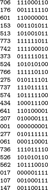
The keys (left) that we use in the examples in this chapter are 3-digit octal numbers, which we also interpret as 9-bit binary values (right).
Figure 16.1 Binary representation of octal keys
The tree depicted in Figure 16.2 is an abstract device-independent representation of an index that is similar to many other data structures that we have considered. Note that, in addition, it is not far removed from device-dependent indexes that might be found in low-level disk access software. For example, some early systems used a two-level scheme, where the bottom level corresponded to the items on the pages for a particular disk device, and the second level corresponded to a master index to the individual devices. In such systems, the master index was kept in main memory, so accessing an item with such an index required two disk accesses: one to get the index, and one to get the page containing the item. As disk capacity increases, so increases the size of the index, and several pages might be required to store the index, eventually leading to a hierarchical scheme like the one depicted in Figure 16.2. We shall continue working with an abstract representation, secure in the knowledge that it can be implemented directly with typical low-level system hardware and software.
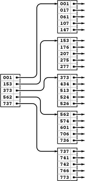
In a sequential index, we keep the keys in sequential order in full pages (right), with an index directing us to the smallest key in each page (left). To add a key, we need to rebuild the data structure.
Figure 16.2 Indexed sequential file structure
Many modern systems use a similar tree structure to organize huge files as a sequence of disk pages. Such trees contain no keys, but they can efficiently support the commonly used operations of accessing the file in sequential order, and, if each node contains a count of its tree size, of finding the page containing the kth item in the file.
Historically, because it combines a sequential key organization with indexed access, the indexing method depicted in Figure 16.2 is called indexed sequential access. It is the method of choice for applications in which changes to the database are rare. We sometimes refer to the index itself as a directory. The disadvantage of using indexed sequential access is that modifying the directory is an expensive operation. For example, adding a single key can require rebuilding virtually the whole database, with new positions for many of the keys and new values for the indexes. To combat this defect and to provide for modest growth, early systems provided for overflow pages on disks and overflow space in pages, but such techniques ultimately were not very effective in dynamic situations (see Exercise 16.3). The methods that we consider in Sections 16.3 and 16.4 provide systematic and efficient alternatives to such ad hoc schemes.
Property 16.1 A search in an indexed sequential file requires only a constant number of probes, but an insertion can involve rebuilding the entire index.
We use the term constant loosely here (and throughout this chapter) to refer to a quantity that is proportional to logM N for large M. As we have discussed, this usage is justified for practical file sizes. Figure 16.3 gives more examples. Even if we were to have a 128-bit search key, capable of specifying the impossibly large number of 2128 different items, we could find an item with a given key in 13 probes, with 1000-way branching. ![]()

These generous upper bounds indicate that we can assume safely, for practical purposes, that we will never have a symbol table with more than 1030 items. Even in such an unrealistically huge database, we could find an item with a given key with less than 10 probes, if we did 1000-way branching. Even if we somehow found a way to store information on each electron in the universe, 1000-way branching would give us access to any particular item with less than 27 probes.
Figure 16.3 Examples of data set sizes
We will not consider implementations that search and construct indexes of this type, because they are special cases of the more general mechanisms that we consider in Section 16.3 (see Exercise 16.17 and Program 16.2).
Exercises
![]() 16.1 Tabulate the values of logM N, for M = 10, 100, and 1000 and N = 103, 104, 105, and 106.
16.1 Tabulate the values of logM N, for M = 10, 100, and 1000 and N = 103, 104, 105, and 106.
![]() 16.2 Draw an indexed sequential file structure for the keys
16.2 Draw an indexed sequential file structure for the keys 516, 177, 143, 632, 572, 161, 774, 470, 411, 706, 461, 612, 761, 474, 774, 635, 343, 461, 351, 430, 664, 127, 345, 171, and 357, for M = 5 and M = 6.
![]() 16.3 Suppose that we build an indexed sequential file structure for N items in pages of capacity M, but leave k empty spaces in each page for expansion. Give a formula for the number of probes needed for a search, as a function of N, M, and k. Use the formula to determine the number of probes needed for a search when k = M/10, for M = 10, 100, and 1000 and N = 103, 104, 105, and 106.
16.3 Suppose that we build an indexed sequential file structure for N items in pages of capacity M, but leave k empty spaces in each page for expansion. Give a formula for the number of probes needed for a search, as a function of N, M, and k. Use the formula to determine the number of probes needed for a search when k = M/10, for M = 10, 100, and 1000 and N = 103, 104, 105, and 106.
![]() 16.4 Suppose that the cost of a probe is about α time units, and that the average cost of finding an item in a page is about βM time units. Find the value of M that minimizes the cost for a search in an indexed sequential file structure, for α/β = 10, 100, and 1000 and N = 103, 104, 105, and 106.
16.4 Suppose that the cost of a probe is about α time units, and that the average cost of finding an item in a page is about βM time units. Find the value of M that minimizes the cost for a search in an indexed sequential file structure, for α/β = 10, 100, and 1000 and N = 103, 104, 105, and 106.
16.3 B Trees
To build search structures that can be effective in a dynamic situation, we build multiway trees, but we relax the restriction that every node must have exactly M entries. Instead, we insist that every node must have at most M entries, so that they will fit on a page, but we allow nodes to have fewer entries. To be sure that nodes have a sufficient number of entries to provide the branching that we need to keep search paths short, we also insist that all nodes have at least (say) M/2 entries, except possibly the root, which must have a least one entry (two links). The reason for the exception at the root will become clear when we consider the construction algorithm in detail. Such trees were named B trees by Bayer and McCreight, who, in 1970, were the first researchers to consider the use of multiway balanced trees for external searching. Many people reserve the term B tree to describe the exact data structure built by the algorithm suggested by Bayer and McCreight; we use it as a generic term to refer to a family of related algorithms.
We have already seen a B-tree implementation: In Definitions 13.1 and 13.2, we see that B trees of order 4, where each node has at most four links and at least two links, are none other than the balanced 2-3-4 trees of Chapter 13. Indeed, the underlying abstraction generalizes in a straightforward manner, and we can implement B trees by generalizing the top-down 2-3-4 tree implementations in Section 13.4. However, the various differences between external and internal searching that we discussed in Section 16.1 lead us to a number of different implementation decisions. In this section, we consider an implementation that
• Generalizes 2-3-4 trees to trees with between M/2 and M nodes
• Represents multiway nodes with an array of items and links
• Implements an index instead of a search structure containing the items
• Splits from the bottom up
• Separates the index from the items
The final two properties in this list are not essential, but are convenient in many situations and are normally found in B tree implementations.
Figure 16.4 illustrates an abstract 4-5-6-7-8 tree, which generalizes the 2-3-4 tree that we considered in Section 13.3. The generalization is straightforward: 4-nodes have three keys and four links, 5-nodes have four keys and five links, and so forth, with one link for each possible interval between keys. To search, we start at the root and move from one node to the next by finding the proper interval for the search key in the current node and then exiting through the corresponding link to get to the next node. We terminate the search with a search hit if we find the search key in any node that we touch; we terminate with a search miss if we reach the bottom of the tree without a hit. As we can in top-down 2-3-4 trees, we can insert a new key at the bottom of the tree after a search if, on the way down the tree, we split nodes that are full: If the root is an 8-node, we split it into a 2-node connected to two 4-nodes; then, any time we see a k-node attached to an 8-node, we replace it by a (k + 1)-node attached to two 4-nodes. This policy guarantees that we have room to insert the new node when we reach the bottom.
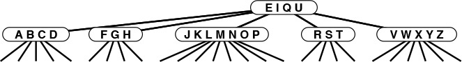
This figure depicts a generalization of 2-3-4 trees built from nodes with 4 through 8 links (and 3 through 7 keys, respectively). As with 2-3-4 trees, we keep the height constant by splitting 8-nodes when encountering them, with either a top-down or a bottom-up insertion algorithm. For example, to insert another J into this tree, we would first split the 8-node into two 4-nodes, then insert the M into the root, converting it into a 6-node. When the root splits, we have no choice but to create a new root that is a 2-node, so the root node is excused from the constraint that nodes must have at least four links.
Figure 16.4 A 4-5-6-7-8 tree
Alternatively, as discussed for 2-3-4 trees in Section 13.3, we can split from the bottom up: We insert by searching and putting the new key in the bottom node, unless that node is a 8-node, in which case we split it into two 4-nodes and insert the middle key and the links to the two new nodes into its parent, working up the tree until encountering an ancestor that is not a 8-node.
Replacing 4 by M/2 and 8 by M in descriptions in the previous two paragraphs converts them into descriptions of search and insert for M/2-...-M trees, for any positive even integer M, even 2 (see Exercise 16.9).
Definition 16.2 A B tree of order M is a tree that either is empty or comprises k-nodes, with k − 1 keys and k links to trees representing each of the k intervals delimited by the keys, and has the following structural properties: k must be between 2 and M at the root and between M/2 and M at every other node; and all links to empty trees must be at the same distance from the root.
B tree algorithms are built upon this basic set of abstractions. As in Chapter 13, we have a great deal of freedom in choosing concrete representations for such trees. For example, we can use an extended red-black representation (see Exercise 13.69). For external searching, we use the even more straightforward ordered-array representation, taking M to be sufficiently large that M-nodes fill a page. The branching factor is at least M/2, so the number of probes for any search or insert is effectively constant, as discussed following Property 16.1.
Instead of implementing the method just described, we consider a variant that generalizes the standard index that we considered in Section 16.1. We keep keys with item references in external pages at the bottom of the tree, and copies of keys with page references in internal pages. We insert new items at the bottom, and then use the basic M/2-...-M tree abstraction. When a page has M entries, we split it into two pages with M/2 pages each, and insert a reference to the new page into its parent. When the root splits, we make a new root with two children, thus increasing the height of the tree by 1.
Figures 16.5 through 16.7 show the B tree that we build by inserting the keys in Figure 16.1 (in the order given) into an initially empty tree, with M = 5. Doing insertions involves simply adding an item to a page, but we can look at the final tree structure to determine the significant events that occurred during its construction. It has seven external pages, so there must have been six external node splits, and it is of height 3, so the root of the tree must have split twice. These events are described in the commentary that accompanies the figures.
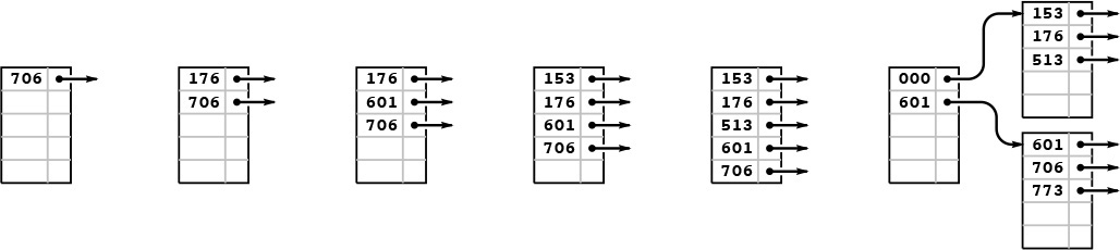
This example shows six insertions into an initially empty B tree built with pages that can hold five keys and links, using keys that are 3-digit octal numbers (9-bit binary numbers). We keep the keys in order in the pages. The sixth insertion causes a split into two external nodes with three keys each and an internal node that serves as an index: Its first pointer points to the page containing all keys greater than or equal to 000 but less than 601, and its second pointer points to the page containing all keys greater than or equal to 601.
Figure 16.5 B tree construction, part 1

After we insert the four keys 742, 373, 524, and 766 into the rightmost B tree in Figure 16.5, both of the external pages are full (left). Then, when we insert 275, the first page splits, sending a link to the new page (along with its smallest key 373) up to the index (center); when we then insert 737, the page at the bottom splits, again sending a link to the new page up to the index (right).
Figure 16.6 B tree construction, part 2

Continuing our example, we insert the 13 keys 574, 434, 641, 207, 001, 277, 061, 736, 526, 562, 017, 107, and 147 into the rightmost B tree in Figure 16.6. Node splits occur when we insert 277 (left), 526 (center), and 107 (right). The node split caused by inserting 526 also causes the index page to split, and increases the height of the tree by one.
Figure 16.7 B tree construction, part 3
Program 16.1 gives the type definitions for nodes and the initialization code for our B-tree implementation. It is similar to several other tree-search implementations that we have examined, in Chapters 13 and 15. The chief added wrinkle is that we use the C union construct to allow us to define slightly different external and internal nodes with the same structure (and the same type of link): Each node consists of an array of keys with associated links (in internal nodes) or items (in external nodes), and a count giving the number of active entries.
With these definitions and the example trees that we just considered, the code for search that is given in Program 16.2 is straightforward. For external nodes, we scan through the array of nodes to look for a key matching the search key, returning the associated item if we succeed and a null item if we do not. For internal nodes, we scan through the array of nodes to find the link to the unique subtree that could contain the search key.
Program 16.3 is an implementation of insert for B trees; it too uses the recursive approach that we have taken for numerous other search-tree implementations in Chapters 13 and 15. It is a bottom-up implementation because we check for node splitting after the recursive call, so the first node split is an external node. The split requires that we pass up a new link to the parent of the split node, which in turn might need to split and pass up a link to its parent, and so forth, perhaps all the way up to the root of the tree (when the root splits, we create a new root, with two children). By contrast, the 2-3-4–tree implementation of Program 13.6 checks for splits before the recursive call, so we do splitting on the way down the tree. We could also use a top-down approach for B trees (see Exercise 16.10). This distinction between top-down versus bottom-up approaches is unimportant in many B tree applications, because the trees are so flat.
The node-splitting code is given in Program 16.4. In the code, we use an even value for the variable M, and we allow only M − 1 items per node in the tree. This policy allows us to insert the Mth item into a node before splitting that node, and simplifies the code considerably without having much effect on the cost (see Exercises 16.20 and 16.21). For simplicity, we use the upper bound of M items per node in the analytic results later in this section; the actual differences are minute. In a top-down implementation, we would not have to resort to this technique, because the convenience of being sure that there is always room to insert a new key in each node comes automatically.
Property 16.2 A search or an insertion in a B tree of order M with N items requires between logM N and logM/2 N probes—a constant number, for practical purposes.
This property follows from the observation that all the nodes in the interior of the B tree (nodes that are not the root and are not external) have between M/2 and M links, since they are formed from a split of a full node with M keys, and can only grow in size (when a lower node is split). In the best case, these nodes form a complete tree of degree M, which leads immediately to the stated bound (see Property 16.1). In the worst case, we have a complete tree of degree M/2. ![]()
When M is 1000, the height of the tree is less than three for N less than 125 million. In typical situations, we can reduce the cost to two probes by keeping the root node in internal memory. For a disk-searching implementation, we might take this step explicitly before embarking on any application involving a huge number of searches; in a virtual memory with caching, the root node will be the one most likely to be in fast memory, because it is the most frequently accessed node.
We can hardly expect to have a search implementation that can guarantee a cost of fewer than two probes for search and insert in huge files, and B trees are widely used because they allow us to achieve this ideal. The price of this speed and flexibility is the empty space within the nodes, which could be a liability for huge files.
Property 16.3 A B tree of order M constructed from N random items is expected to have about 1.44N/M pages.
Yao proved this fact in 1979, using mathematical analysis that is beyond the scope of this book (see reference section). It is based on analyzing a simple probabilistic model that describes tree growth. After the first M/2 nodes have been inserted, there are, at any given time, ti external pages with i items, for M/2 ≤ i ≤ M, with tM/2 + ... + tM = N. Since each interval between nodes is equally likely to receive a random key, the probability that a node with i items is hit is ti/N. Specifically, for i < M, this quantity is the probability that the number of external pages with i items decreases by 1 and the number of external pages with (i + 1) items increases by 1; and for i = 2M, this quantity is the probability that the number of external pages with 2M items decreases by 1 and the number of external pages with M items increases by 2. Such a probabilistic process is called a Markov chain. Yao’s result is based on an analysis of the asymptotic properties of this chain. ![]()
We can also validate Property 16.3 by writing a program to simulate the probabilistic process (see Exercise 16.11 and Figures 16.8 and 16.9). Of course, we also could just build random B trees and measure their structural properties. The probabilistic simulation is simpler to do than either the mathematical analysis or the full implementation, and is an important tool for us to use in studying and comparing variants of the algorithm (see, for example, Exercise 16.16).

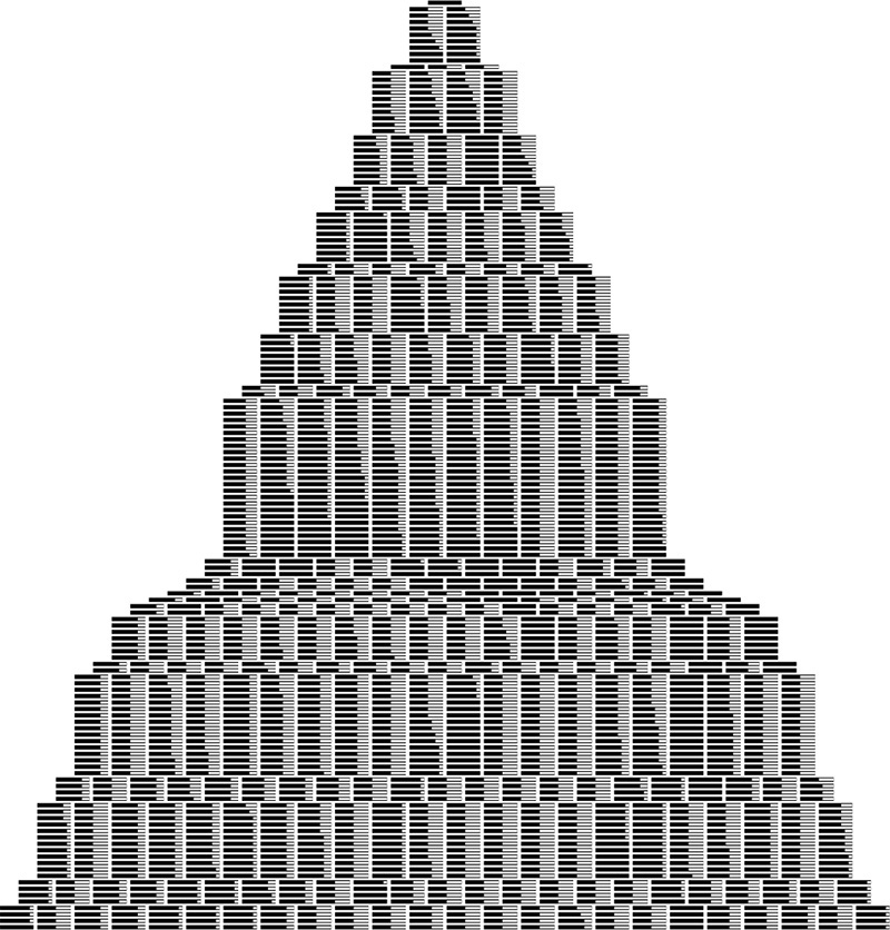
In this simulation, we insert items with random keys into an initially empty B tree with pages that can hold nine keys and links. Each line displays the external nodes, with each external node depicted as a line segment of length proportional to the number of items in that node. Most insertions land in an external node that is not full, increasing that node’s size by 1. When an insertion lands in a full external node, the node splits into two nodes of half the size.
Figure 16.8 Growth of a large B tree
This version of Figure 16.8 shows how pages fill during the B tree growth process. Again, most insertions land in a page that is not full and just increase its occupancy by 1. When an insertion does land in a full page, the page splits into two half-empty pages.
Figure 16.9 Growth of a large B tree, page occupancy exposed
The implementations of other symbol-table operations are similar to those for several other tree-based representations that we have seen before, and are left as exercises (see Exercises 16.22 through 16.25). In particular, select and sort implementations are straightforward, but as usual, implementing a proper delete can be a challenging task. Like insert, most delete operations are a simple matter of removing an item from an external page and decrementing its counter, but what do we do when we have to remove an item from a node that has only M/2 items? The natural approach is to find items from sibling nodes to fill the space (perhaps reducing the number of nodes by one), but the implementation becomes complicated because we have to track down the keys associated with any items that we move among nodes. In practical situations, we can typically adopt the much simpler approach of letting external nodes become underfull, without suffering much performance degradation (see Exercise 16.25).
Many variations on the basic B-tree abstraction suggest themselves immediately. One class of variations saves time by packing as many page references as possible in internal nodes, thereby increasing the branching factor and flattening the tree. As we have discussed, the benefits of such changes are marginal in modern systems, since standard values of the parameters allow us to implement search and insert with two probes—an efficiency that we could hardly improve. Another class of variations improves storage efficiency by combining nodes with siblings before splitting. Exercises 16.13 through 16.16 are concerned with such a method, which reduces the excess storage used from 44 to 23 per cent, for random keys. As usual, the proper choice among different variations depends on properties of applications. Given the broad variety of different situations where B trees are applicable, we will not consider such issues in detail. We also will not be able to consider details of implementations, because there are so many device- and system-dependent matters to take into account. As usual, delving deeply into such implementations is a risky business, and we shy away from such fragile and nonportable code in modern systems, particularly when the basic algorithm performs so well.
Exercises
![]() 16.5 Give the contents of the 3-4-5-6 tree that results when you insert the keys E A S Y Q U E S T I O N W I T H P L E N T Y O F K E Y S in that order into an initially empty tree.
16.5 Give the contents of the 3-4-5-6 tree that results when you insert the keys E A S Y Q U E S T I O N W I T H P L E N T Y O F K E Y S in that order into an initially empty tree.
![]() 16.6 Draw figures corresponding to Figures 16.5 through 16.7, to illustrate the process of inserting the keys
16.6 Draw figures corresponding to Figures 16.5 through 16.7, to illustrate the process of inserting the keys 516, 177, 143, 632, 572, 161, 774, 470, 411, 706, 461, 612, 761, 474, 774, 635, 343, 461, 351, 430, 664, 127, 345, 171, and 357 in that order into an initially empty tree, with M = 5.
![]() 16.7 Give the height of the B trees that result when you insert the keys in Exercise 16.28 in that order into an initially empty tree, for each value of M > 2.
16.7 Give the height of the B trees that result when you insert the keys in Exercise 16.28 in that order into an initially empty tree, for each value of M > 2.
16.8 Draw the B tree that results when you insert 16 equal keys into an initially empty tree, with M = 4.
![]() 16.9 Draw the 1-2 tree that results when you insert the keys E A S Y Q U E S T I O N into an initially empty tree. Explain why 1-2 trees are not of practical interest as balanced trees.
16.9 Draw the 1-2 tree that results when you insert the keys E A S Y Q U E S T I O N into an initially empty tree. Explain why 1-2 trees are not of practical interest as balanced trees.
![]() 16.10 Modify the B-tree–insertion implementation in Program 16.3 to do splitting on the way down the tree, in a manner similar to our implementation of 2-3-4–tree insertion (Program 13.6).
16.10 Modify the B-tree–insertion implementation in Program 16.3 to do splitting on the way down the tree, in a manner similar to our implementation of 2-3-4–tree insertion (Program 13.6).
![]() 16.11 Write a program to compute the average number of external pages for a B tree of order M built from N random insertions into an initially empty tree, using the probabilistic process described after Property 16.1. Run your program for M = 10, 100, and 1000 and N = 103, 104, 105, and 106.
16.11 Write a program to compute the average number of external pages for a B tree of order M built from N random insertions into an initially empty tree, using the probabilistic process described after Property 16.1. Run your program for M = 10, 100, and 1000 and N = 103, 104, 105, and 106.
![]() 16.12 Suppose that, in a three-level tree, we can afford to keep a links in internal memory, between b and 2b links in pages representing internal nodes, and between c and 2c items in pages representing external nodes. What is the maximum number of items that we can hold in such a tree, as a function of a, b, and c?
16.12 Suppose that, in a three-level tree, we can afford to keep a links in internal memory, between b and 2b links in pages representing internal nodes, and between c and 2c items in pages representing external nodes. What is the maximum number of items that we can hold in such a tree, as a function of a, b, and c?
![]() 16.13 Consider the sibling split (or B* tree) heuristic for B trees: When it comes time to split a node because it contains M entries, we combine the node with its sibling. If the sibling has k entries with k < M – 1, we reallocate the items giving the sibling and the full node each about (M + k)/2 entries. Otherwise, we create a new node and give each of the three nodes about 2M/3 entries. Also, we allow the root to grow to hold about 4M/3 items, splitting it and creating a new root node with two entries when it reaches that bound. State bounds on the number of probes used for a search or an insertion in a B* tree of order M with N items. Compare your bounds with the corresponding bounds for B trees (see Property 16.2), for M = 10, 100, and 1000 and N = 103, 104, 105, and 106.
16.13 Consider the sibling split (or B* tree) heuristic for B trees: When it comes time to split a node because it contains M entries, we combine the node with its sibling. If the sibling has k entries with k < M – 1, we reallocate the items giving the sibling and the full node each about (M + k)/2 entries. Otherwise, we create a new node and give each of the three nodes about 2M/3 entries. Also, we allow the root to grow to hold about 4M/3 items, splitting it and creating a new root node with two entries when it reaches that bound. State bounds on the number of probes used for a search or an insertion in a B* tree of order M with N items. Compare your bounds with the corresponding bounds for B trees (see Property 16.2), for M = 10, 100, and 1000 and N = 103, 104, 105, and 106.
![]() 16.14 Develop a B* tree insert implementation (based on the sibling-split heuristic).
16.14 Develop a B* tree insert implementation (based on the sibling-split heuristic).
![]() 16.15 Create a figure like Figure 16.8 for the sibling-split heuristic.
16.15 Create a figure like Figure 16.8 for the sibling-split heuristic.
![]() 16.16 Run a probabilistic simulation (see Exercise 16.11) to determine the average number of pages used when we use the sibling-split heuristic, building a B* tree of order M by inserting random nodes into an initially empty tree, for M = 10, 100, and 1000 and N = 103, 104, 105, and 106.
16.16 Run a probabilistic simulation (see Exercise 16.11) to determine the average number of pages used when we use the sibling-split heuristic, building a B* tree of order M by inserting random nodes into an initially empty tree, for M = 10, 100, and 1000 and N = 103, 104, 105, and 106.
![]() 16.17 Write a program to construct a B tree index from the bottom up, starting with an array of pointers to pages containing between M and 2M items, in sorted order.
16.17 Write a program to construct a B tree index from the bottom up, starting with an array of pointers to pages containing between M and 2M items, in sorted order.
![]() 16.18 Could an index with all pages full, such as Figure 16.2, be constructed by the B-tree–insertion algorithm considered in the text (Program 16.3)? Explain your answer.
16.18 Could an index with all pages full, such as Figure 16.2, be constructed by the B-tree–insertion algorithm considered in the text (Program 16.3)? Explain your answer.
16.19 Suppose that many different computers have access to the same index, so several programs may be trying to insert a new node in the same B tree at about the same time. Explain why you might prefer to use top-down B trees instead of bottom-up B trees in such a situation. Assume that each program can (and does) delay the others from modifying any given node that it has read and might later modify.
![]() 16.20 Modify the B-tree implementation in Programs 16.1 through 16.3 to allow M items per node to exist in the tree.
16.20 Modify the B-tree implementation in Programs 16.1 through 16.3 to allow M items per node to exist in the tree.
![]() 16.21 Tabulate the difference between log999 N and log1000 N, for N = 103,104, 105, and 106.
16.21 Tabulate the difference between log999 N and log1000 N, for N = 103,104, 105, and 106.
![]() 16.22 Implement the sort operation for a B-tree–based symbol table.
16.22 Implement the sort operation for a B-tree–based symbol table.
![]() 16.23 Implement the select operation for a B-tree–based symbol table.
16.23 Implement the select operation for a B-tree–based symbol table.
![]() 16.24 Implement the delete operation for a B-tree–based symbol table.
16.24 Implement the delete operation for a B-tree–based symbol table.
![]() 16.25 Implement the delete operation for a B-tree–based symbol table, using a simple method where you delete the indicated item from its external page (perhaps allowing the number of items in the page to fall below M/2), but do not propagate the change up through the tree, except possibly to adjust the key values if the deleted item was the smallest in its page.
16.25 Implement the delete operation for a B-tree–based symbol table, using a simple method where you delete the indicated item from its external page (perhaps allowing the number of items in the page to fall below M/2), but do not propagate the change up through the tree, except possibly to adjust the key values if the deleted item was the smallest in its page.
![]() 16.26 Modify Programs 16.2 and 16.3 to use binary search (see Program 12.6) within nodes. Determine the value of M that minimizes the time that your program takes to build a symbol table by inserting N items with random keys into an initially empty table, for N = 103, 104, 105, and 106, and compare the times that you get with the corresponding times for red–black trees (Program 13.6).
16.26 Modify Programs 16.2 and 16.3 to use binary search (see Program 12.6) within nodes. Determine the value of M that minimizes the time that your program takes to build a symbol table by inserting N items with random keys into an initially empty table, for N = 103, 104, 105, and 106, and compare the times that you get with the corresponding times for red–black trees (Program 13.6).
16.4 Extendible Hashing
An alternative to B trees that extends digital searching algorithms to apply to external searching was developed in 1978 by Fagin, Nievergelt, Pippenger, and Strong. Their method, called extendible hashing, leads to a search implementation that requires just one or two probes for typical applications. The corresponding insert implementation also (almost always) requires just one or two probes.
Extendible hashing combines features of hashing, multiway-trie algorithms, and sequential-access methods. Like the hashing methods of Chapter 14, extendible hashing is a randomized algorithm—the first step is to define a hash function that transforms keys into integers (see Section 14.1). For simplicity, in this section, we simply consider keys to be random fixed-length bitstrings. Like the multiway-trie algorithms of Chapter 15, extendible hashing begins a search by using the leading bits of the keys to index into a table whose size is a power of 2. Like B-tree algorithms, extendible hashing stores items on pages that are split into two pieces when they fill up. Like indexed sequential-access methods, extendible hashing maintains a directory that tells us where we can find the page containing the items that match the search key. The blending of these familiar features in one algorithm makes extendible hashing a fitting conclusion to our study of search algorithms.
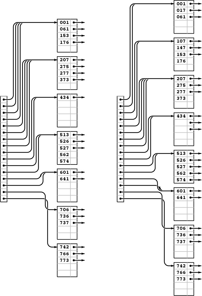
Suppose that the number of disk pages that we have available is a power of 2—say 2d. Then, we can maintain a directory of the 2d different page references, use d bits of the keys to index into the directory, and can keep, on the same page, all keys that match in their first k bits, as illustrated in Figure 16.10. As we do with B trees, we keep the items in order on the pages, and do sequential search once we reach the page corresponding to an item with a given search key.
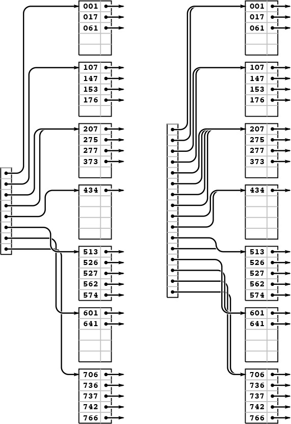
With a directory of eight entries, we can store up to 40 keys by storing all records whose first 3 bits match on the same page, which we can access via a pointer stored in the directory (left). Directory entry 0 contains a pointer to the page that contains all keys that begin with 000; table entry 1 contains a pointer to the page that contains all keys that begin with 001; table entry 2 contains a pointer to the page that contains all keys that begin with 010, and so forth. If some pages are not fully populated, we can reduce the number of pages required by having multiple directory pointers to a page. In this example (left), 373 is on the same page as the keys that start with 2; that page is defined to be the page that contains items with keys whose first 2 bits are 01.
If we double the size of the directory and clone each pointer, we get a structure that we can index with the first 4 bits of the search key (right). For example, the final page is still defined to be the page that contains items with keys whose first three bits are 111, and it will be accessed through the directory if the first 4 bits of the search key are 1110 or 1111. This larger directory can accommodate growth in the table.
Figure 16.10 Directory page indices
Figure 16.10 illustrates the two basic concepts behind extendible hashing. First, we do not necessarily need to maintain 2d pages. That is, we can arrange to have multiple directory entries refer to the same page, without changing our ability to search the structure quickly, by combining keys with differing values for their leading d bits together on the same page, while still maintaining our ability to find the page containing a given key by using the leading bits of the key to index into the directory. Second, we can double the size of the directory to increase the capacity of the table.
Specifically, the data structure that we use for extendible hashing is much simpler than the one that we used for B trees. It consists of pages that contain up to M items, and a directory of 2d pointers to pages (see Program 16.5). The pointer in directory location x refers to the page that contains all items whose leading d bits are equal to x. The table is constructed with d sufficiently large that we are guaranteed that there are less than M items on each page. The implementation of search is simple: We use the leading d bits of the key to index into the directory, which gives us access to the page that contains any items with matching keys, then do sequential search for such an item on that page (see Program 16.6).
The data structure needs to become slightly more complicated to support insert, but one of its essential features is that this search algorithm works properly without any modification. To support insert, we need to address the following questions:
• What do we do when the number of items that belong on a page exceeds that page’s capacity?
• What directory size should we use?
For example, we could not use d = 2 in the example in Figure 16.10 because some pages would overflow, and we would not use d = 5 because too many pages would be empty. As usual, we are most interested in supporting the insert operation for the symbol-table ADT, so that, for example, the structure can grow gradually as we do a series of intermixed search and insert operations. Taking this point of view corresponds to refining our first question:
• What do we do when we need to insert an item into a full page?
For example, we could not insert an item whose key starts with a 5 or a 7 in the example in Figure 16.10 because the corresponding pages are full.
Definition 16.3 An extendible hash table of order d is a directory of 2d references to pages that contain up to M items with keys. The items on each page are identical in their first k bits, and the directory contains 2d−k pointers to the page, starting at the location specified by the leading k bits in the keys on the page.
Some d-bit patterns may not appear in any keys. We leave the corresponding directory entries unspecified in Definition 16.3, although there is a natural way to organize pointers to null pages; we will examine it shortly.
To maintain these characteristics as the table grows, we use two basic operations: a page split, where we distribute some of the keys from a full page onto another page; and a directory split, where we double the size of the directory and increase d by 1. Specifically, when a page fills, we split it into two pages, using the leftmost bit position for which the keys differ to decide which items go to the new page. When a page splits, we adjust the directory pointers appropriately, doubling the size of the directory if necessary.
As usual, the best way to understand the algorithm is to trace through its operation as we insert a set of keys into an initially empty table. Each of the situations that the algorithm must address occurs early in the process, in a simple form, and we soon come to a realization of the algorithm’s underlying principles. Figures 16.11 through 16.13 show the construction of an extendible hash table for the sample set of 25 octal keys that we have been considering in this chapter. As occurs in B trees, most of the insertions are uneventful: They simply add a key to a page. Since we start with one page and end up with eight pages, we can infer that seven of the insertions caused a page split; since we start with a directory of size 1 and end up with a directory of size 16, we can infer that four of the insertions caused a directory split.
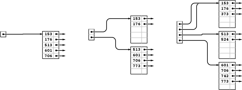
As in B trees, the first five insertions into an extendible hash table go into a single page (left). Then, when we insert 773, we split into two pages (one with all the keys beginning with a 0 bit and one with all the keys beginning with a 1 bit) and double the size of the directory to hold one pointer to each of the pages (center). We insert 742 into the bottom page (be-cause it begins with a 1 bit) and 373 into the top page (because it begins with a 0 bit), but we then need to split the bottom page to accommodate 524. For this split, we put all the items with keys that begin with 10 on one page and all the items with keys that begin with 11 on the other, and we again double the size of the directory to accommodate pointers to both of these pages (right). The directory contains two pointers to the page containing items with keys starting with a 0 bit: one for keys that begin with 00 and the other for keys that begin with 01.
Figure 16.11 Extendible hash table construction, part 1
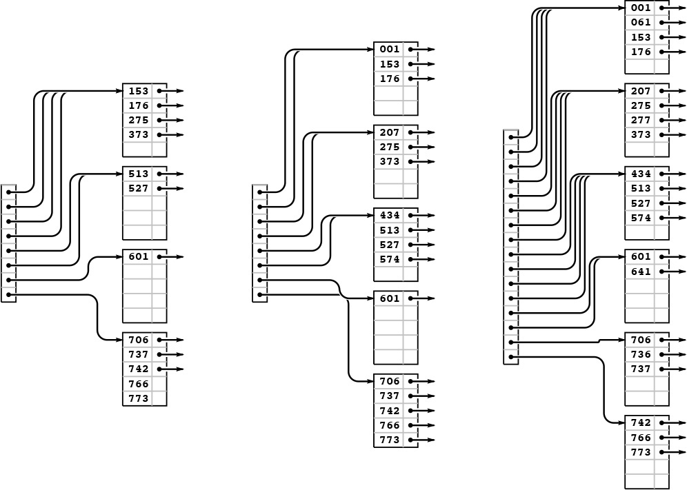
We insert the keys 766 and 275 into the rightmost B tree in Figure 16.11 without any node splits (left). Then, when we insert 737, the bottom page splits, and that, because there is only one link to the bottom page, causes a directory split (center). Then, we insert 574, 434, 641, and 207 before 001 causes the top page to split (right).
Figure 16.12 Extendible hash table construction, part 2
Continuing the example in Figures 16.11 and 16.12, we insert the 5 keys 526, 562, 017, 107, and 147 into the rightmost B tree in Figure 16.6. Node splits occur when we insert 526 (left) and 107 (right).
Figure 16.13 Extendible hash table construction, part 3
Property 16.4 The extendible hash table built from a set of keys depends on only the values of those keys, and does not depend on the order in which the keys are inserted.
Consider the trie corresponding to the keys (see Property 15.2), with each internal node labeled with the number of items in its subtree. An internal node corresponds to a page in the extendible hash table if and only if its label is less than M and its parent’s label is not less than M. All the items below the node go on that page. If a node is at level k, it corresponds to a k-bit pattern derived from the trie path in the normal way, and all entries in the extendible hash table’s directory with indices that begin with that k-bit pattern contain pointers to the corresponding page. The size of the directory is determined by the deepest level among all the internal nodes in the trie that correspond to pages. Thus, we can convert a trie to an extendible hash table without regard to the order in which items are inserted, and this property holds as a consequence of Property 15.2. ![]()
Program 16.7 is an implementation of the insert operation for an extendible hash table. First, we access the page that could contain the search key, with a single reference to the directory, as we did for search. Then, we insert the new item there, as we did for external nodes in B trees (see Program 16.2). If this insertion leaves M items in the node, then we invoke a split function, again as we did for B trees, but the split function is more complicated in this case. Each page contains the number k of leading bits that we know to be the same in the keys of all the items on the page, and, because we number bits from the left starting at 0, k also specifies the index of the bit that we want to test to determine how to split the items.
Therefore, to split a page, we make a new page, then put all the items for which that bit is 0 on the old page and all the items for which that bit is 1 on the new page, then set the bit count to k +1 for both pages. Now, it could be the case that all the keys have the same value for bit k, which would still leave us with a full node. If so, we simply go on to the next bit, continuing until we get a least one item in each page. The process must terminate, eventually, unless we have M values of the same key. We discuss that case shortly.
As with B trees, we leave space for an extra entry in every page to allow splitting after insertion, thus simplifying the code. Again, this technique has little practical effect, and we can ignore the effect in the analysis.
When we create a new page, we have to insert a pointer to it in the directory. The code that accomplishes this insertion is given in Program 16.8. The simplest case to consider is the one where the directory, prior to insertion, has precisely two pointers to the page that splits. In that case, we need simply to arrange to set the second pointer to reference the new page. If the number of bits k that we need to distinguish the keys on the new page is greater than the number of bits d that we have to access the directory, then we have to increase the size of the directory to accommodate the new entry. Finally, we update the directory pointers as appropriate.
If more than M items have duplicate keys, the table overflows, and the code in Program 16.7 goes into an infinite loop, looking for a way to distinguish the keys. A related problem is that the directory may get unnecessarily huge, if the keys have an excessive number of leading bits that are equal. This situation is akin to the excessive time required for MSD radix sort, for files that have large numbers of duplicate keys or long stretches of bit positions where they are identical. We depend on the randomization provided by the hash function to stave off these problems (see Exercise 16.43). Even with hashing, extraordinary steps must be taken if large numbers of duplicate keys are present, because hash functions take equal keys to equal hash values. Duplicate keys can make the directory artificially large; and the algorithm breaks down entirely if there are more equal keys than fit in one page. Therefore, we need to add tests to guard against the occurrence of these conditions before using this code (see Exercise 16.35).
The primary performance parameters of interest are the number of pages used (as with B trees) and the size of the directory. The randomization for this algorithm is provided by the hash functions, so average-case performance results apply to any sequence of N distinct insertions.
Property 16.5 With pages that can hold M items, extendible hashing requires about 1.44(N/M) pages for a file of N items, on the average. The expected number of entries in the directory is about 3.92(N1/M)(N/M).
This (rather deep) result extends the analysis of tries that we discussed briefly in the previous chapter (see reference section). The exact constants are lg e = 1/ ln 2 for the number of pages and e lg e = e/ ln 2 for the directory size, though the precise values of the quantities oscillate around these average values. We should not be surprised by this phenomenon because, for example, the directory size has to be a power of 2, a fact which has to be accounted for in the result. ![]()
Note that the growth rate of the directory size is faster than linear in N, particularly for small M. However, for N and M in ranges of practical interest, N1/M is quite close to 1, so we can expect the directory to have about 4(N/M) entries, in practice.
We have considered the directory to be a single array of pointers. We can keep the directory in memory, or, if it is too big, we can keep a root node in memory that tells where the directory pages are, using the same indexing scheme. Alternatively, we can add another level, indexing the first level on the first 10 bits (say), and the second level on the rest of the bits (see Exercise 16.36).
As we did for B trees, we leave the implementation of other symbol-table operations for exercises (see Exercises 16.38 and 16.41). Also as it is with B trees, a proper delete implementation is a challenge, but allowing underfull pages is an easy alternative that can be effective in many practical situations.
Exercises
![]() 16.27 How many pages would be empty if we were to use a directory of size 32 in Figure 16.10?
16.27 How many pages would be empty if we were to use a directory of size 32 in Figure 16.10?
16.28 Draw figures corresponding to Figures 16.11 through 16.13, to illustrate the process of inserting the keys 562, 221, 240, 771, 274, 233, 401, 273, and 201 in that order into an initially empty tree, with M = 5.
![]() 16.29 Draw figures corresponding to Figures 16.11 through 16.13, to illustrate the process of inserting the keys
16.29 Draw figures corresponding to Figures 16.11 through 16.13, to illustrate the process of inserting the keys 562, 221, 240, 771, 274, 233, 401, 273, and 201 in that order into an initially empty tree, with M = 5.
![]() 16.30 Assume that you are given an array of items in sorted order. Describe how you would determine the directory size of the extendible hash table corresponding to that set of items.
16.30 Assume that you are given an array of items in sorted order. Describe how you would determine the directory size of the extendible hash table corresponding to that set of items.
![]() 16.31 Write a program that constructs an extendible hash table from an array of items that is in sorted order, by doing two passes through the items: one to determine the size of the directory (see Exercise 16.30) and one to allocate the items to pages and fill in the directory.
16.31 Write a program that constructs an extendible hash table from an array of items that is in sorted order, by doing two passes through the items: one to determine the size of the directory (see Exercise 16.30) and one to allocate the items to pages and fill in the directory.
![]() 16.32 Give a set of keys for which the corresponding extendible hash table has directory size 16, with eight pointers to a single page.
16.32 Give a set of keys for which the corresponding extendible hash table has directory size 16, with eight pointers to a single page.
![]() 16.33 Create a figure like Figure 16.8 for extendible hashing.
16.33 Create a figure like Figure 16.8 for extendible hashing.
![]() 16.34 Write a program to compute the average number of external pages and the average directory size for an extendible hash table built from N random insertions into an initially empty tree, when the page capacity is M. Compute the percentage of empty space, for M = 10, 100, and 1000 and N = 103, 104, 105, and 106.
16.34 Write a program to compute the average number of external pages and the average directory size for an extendible hash table built from N random insertions into an initially empty tree, when the page capacity is M. Compute the percentage of empty space, for M = 10, 100, and 1000 and N = 103, 104, 105, and 106.
16.35 Add appropriate tests to Program 16.7 to guard against malfunction in case too many duplicate keys or keys with too many leading equal bits are inserted into the table.
![]() 16.36 Modify the extendible-hashing implementation in Programs 16.5 through 16.7 to use a two-level directory, with no more than M pointers per directory node. Pay particular attention to deciding what to do when the directory first grows from one level to two.
16.36 Modify the extendible-hashing implementation in Programs 16.5 through 16.7 to use a two-level directory, with no more than M pointers per directory node. Pay particular attention to deciding what to do when the directory first grows from one level to two.
![]() 16.37 Modify the extendible-hashing implementation in Programs 16.5 through 16.7 to allow M items per page to exist in the data structure.
16.37 Modify the extendible-hashing implementation in Programs 16.5 through 16.7 to allow M items per page to exist in the data structure.
![]() 16.38 Implement the sort operation for an extendible hash table.
16.38 Implement the sort operation for an extendible hash table.
![]() 16.39 Implement the select operation for an extendible hash table.
16.39 Implement the select operation for an extendible hash table.
![]() 16.40 Implement the delete operation for an extendible hash table.
16.40 Implement the delete operation for an extendible hash table.
![]() 16.41 Implement the delete operation for an extendible hash table, using the method indicated in Exercise 16.25.
16.41 Implement the delete operation for an extendible hash table, using the method indicated in Exercise 16.25.
![]() 16.42 Develop a version of extendible hashing that splits pages when splitting the directory, so that each directory pointer points to a unique page. Develop experiments to compare the performance of your implementation to that of the standard implementation.
16.42 Develop a version of extendible hashing that splits pages when splitting the directory, so that each directory pointer points to a unique page. Develop experiments to compare the performance of your implementation to that of the standard implementation.
![]() 16.43 Run empirical studies to determine the number of random numbers that we would expect to generate before finding more than M numbers with the same d initial bits, for M = 10, 100, and 1000, and for 1 ≤ d ≤ 20.
16.43 Run empirical studies to determine the number of random numbers that we would expect to generate before finding more than M numbers with the same d initial bits, for M = 10, 100, and 1000, and for 1 ≤ d ≤ 20.
![]() 16.44 Modify hashing with separate chaining (Program 14.3) to use a hash table of size 2M, and keep items in pages of size 2M. That is, when a page fills, link it to a new empty page, so each hash table entry points to a linked list of pages. Empirically determine the average number of probes required for a search after building a table from N items with random keys, for M = 10, 100, and 1000 and N = 103, 104, 105, and 106.
16.44 Modify hashing with separate chaining (Program 14.3) to use a hash table of size 2M, and keep items in pages of size 2M. That is, when a page fills, link it to a new empty page, so each hash table entry points to a linked list of pages. Empirically determine the average number of probes required for a search after building a table from N items with random keys, for M = 10, 100, and 1000 and N = 103, 104, 105, and 106.
![]() 16.45 Modify double hashing (Program 14.6) to use pages of size 2M, treating accesses to full pages as “collisions.” Empirically determine the average number of probes required for a search after building a table from N items with random keys, for M = 10, 100, and 1000 and N = 103, 104, 105, and 106, using an initial table size of 3N/2M.
16.45 Modify double hashing (Program 14.6) to use pages of size 2M, treating accesses to full pages as “collisions.” Empirically determine the average number of probes required for a search after building a table from N items with random keys, for M = 10, 100, and 1000 and N = 103, 104, 105, and 106, using an initial table size of 3N/2M.
![]() 16.46 Develop a symbol-table implementation using extendible hashing that supports the initialize, count, search, insert, delete, join, select, and sort operations for first-class symbol-table ADTs with client item handles (see Exercises 12.4 and 12.5).
16.46 Develop a symbol-table implementation using extendible hashing that supports the initialize, count, search, insert, delete, join, select, and sort operations for first-class symbol-table ADTs with client item handles (see Exercises 12.4 and 12.5).
16.5 Perspective
The most important application of the methods discussed in this chapter is to construct indexes for huge databases that are maintained on external memory—for example, in disk files. Although the underlying algorithms that we have discussed are powerful, developing a file-system implementation based on B trees or on extendible hashing is a complex task. First, we cannot use the C programs in this section directly—they have to be modified to read and refer to disk files. Second, we have to be sure that the algorithm parameters (page and directory size, for example) are tuned properly to the characteristics of the particular hardware that we are using. Third, we have to pay attention to reliability, and to error detection and correction. For example, we need to be able to check that the data structure is in a consistent state, and to consider how we might proceed to correct any of the scores of errors that might crop up. Systems considerations of this kind are critical—and are beyond the scope of this book.
On the other hand, if we have a programming system that supports virtual memory, we can put to direct use the C implementations that we have considered here in a situation where we have a huge number of symbol-table operations to perform on a huge table. Roughly, each time that we access a page, such a system will put that page in a cache, where references to data on that page are handled efficiently. If we refer to a page that is not in the cache, the system has to read the page from external memory, so we can think of cache misses as roughly equivalent to the probe cost measure that we have been using.
For B trees, every search or insertion references the root, so the root will always be in the cache. Otherwise, for sufficiently large M, typical searches and insertions involve at most two cache misses. For a large cache, there is a good chance that the first page (the child of the root) that is accessed on a search is already in the cache, so the average cost per search is likely to be significantly less than two probes.
For extendible hashing, it is unlikely that the whole directory will be in the cache, so we expect that both the directory access and the page access might involve a cache miss (this case is the worst case). That is, two probes are required for a search in a huge table, one to access the appropriate part of the directory and one to access the appropriate page.
These algorithms form an appropriate subject on which to close our discussion of searching, because, to use them effectively, we need to understand basic properties of binary search, BSTs, balanced trees, hashing, and tries—the basic searching algorithms that we have studied in Chapters 12 through 15. As a group, these algorithms provide us with solutions to the symbol-table implementation problem in a broad variety of situations: they constitute an outstanding example of the power of algorithmic technology.
Exercises
16.47 Modify the B-tree implementation in Section 16.3 (Programs 16.1 through 16.3) to use an ADT for page references.
16.48 Modify the extendible-hashing implementation in Section 16.4 (Programs 16.5 through 16.8) to use an ADT for page references.
16.49 Estimate the average number of probes per search in a B tree for S random searches, in a typical cache system, where the T most-recently-accessed pages are kept in memory (and therefore add 0 to the probe count). Assume that S is much larger than T.
16.50 Estimate the average number of probes per search in an extendible hash table, for the cache model described in Exercise 16.49.
![]() 16.51 If your system supports virtual memory, design and conduct experiments to compare the performance of B trees with that of binary search, for random searches in a huge symbol table.
16.51 If your system supports virtual memory, design and conduct experiments to compare the performance of B trees with that of binary search, for random searches in a huge symbol table.
16.52 Implement a priority-queue ADT that supports construct for a huge number of items, followed by a huge number of insert and delete the maximum operations (see Chapter 9).
16.53 Develop an external symbol-table ADT based on a skip-list representation of B trees (see Exercise 13.80).
![]() 16.54 If your system supports virtual memory, run experiments to determine the value of M that leads to the fastest search times for a B tree implementation supporting random search operations in a huge symbol table. (It may be worthwhile for you to learn basic properties of your system before conducting such experiments, which can be costly.)
16.54 If your system supports virtual memory, run experiments to determine the value of M that leads to the fastest search times for a B tree implementation supporting random search operations in a huge symbol table. (It may be worthwhile for you to learn basic properties of your system before conducting such experiments, which can be costly.)
![]() 16.55 Modify the B-tree implementation in Section 16.3 (Programs 16.1 through 16.3) to operate in an environment where the table resides on external storage. If your system allows nonsequential file access, put the whole table on a single (huge) file, and use offsets within the file in place of pointers in the data structure. If your system allows you to access pages on external devices directly, use page addresses in place of pointers in the data structure. If your system allows both, choose the approach that you determine to be most reasonable for implementing a huge symbol table.
16.55 Modify the B-tree implementation in Section 16.3 (Programs 16.1 through 16.3) to operate in an environment where the table resides on external storage. If your system allows nonsequential file access, put the whole table on a single (huge) file, and use offsets within the file in place of pointers in the data structure. If your system allows you to access pages on external devices directly, use page addresses in place of pointers in the data structure. If your system allows both, choose the approach that you determine to be most reasonable for implementing a huge symbol table.
![]() 16.56 Modify the extendible-hashing implementation in Section 16.4 (Programs 16.5 through 16.8) to operate in an environment where the table resides on external storage. Explain the reasons for the approach that you choose for allocating the directory and the pages to files (see Exercise 16.55).
16.56 Modify the extendible-hashing implementation in Section 16.4 (Programs 16.5 through 16.8) to operate in an environment where the table resides on external storage. Explain the reasons for the approach that you choose for allocating the directory and the pages to files (see Exercise 16.55).