
Atomic-scale computer simulation of functional materials: methodologies and applications
Abstract: Computer modelling techniques have become significantly more valuable in the study of functional materials for energy applications over the past decades. The first section of this chapter reviews the main methodologies that can be used to investigate the defect processes of energy materials. Examples illustrating the application of modelling techniques to (i) ionically conducting complex oxides and (ii) random semiconductor alloys follow. In the final section, we briefly project to the future and discuss issues that might become important in the years to come.
Key words: mathematical modelling, solid oxide fuel cells, classical potential molecular dynamics (MD), random semiconductor alloys, quantum mechanics, static lattice approach
A.1 Introduction
Over the past decades computer-modelling techniques have become significantly more valuable in the study of functional materials for energy applications. We present the main methodologies that can be used to investigate the defect processes of energy materials. This will be followed by examples, which illustrate the application of modelling techniques to (i) ionically conducting complex oxides and (ii) random semiconductor alloys. The example concerned with cathode materials for solid oxide fuel cells will demonstrate how classical potential molecular dynamics calculations can be used in conjunction with experimental studies to reveal the oxygen transport processes of complex oxides. In contrast, the example of random semiconductor alloys employs a quantum mechanical (QM) technique and a static lattice approach. Finally, we briefly project to the future and discuss issues that might become important in the years to come.
A.2 Methodological approaches
Computer simulation predicts the behaviour of a system subject to the constraints of a mathematical model, as implemented in a computer code. The mathematical model consists of a set of governing equations (and hence assumptions) that describe aspects of the real system. A computer model is, however, necessarily a simplification of the real system. The result of a simulation can be an identification or understanding of the physics/chemistry (the processes) that underpin the behaviour of the system – if the right questions/model has been chosen.
There are three essential types of atomic-scale simulations, which attempt to deliver quite different predictions: first, static-type approaches that yield predictions of the relaxed coordinates of ions using energy minimization; second, molecular dynamics (MD) approaches, which predict the motion of ions; third, statistical approaches such as Monte Carlo, that are most commonly used to deliver distributions of atoms. In each case we need to know the forces or energies of interaction between atoms in the ensemble. This can be achieved in two ways: either classical based where effective potentials act between atoms, or QM based, which includes density functional theory (DFT) simulations. These will now all be reviewed in detail.
A.2.1 Energy minimization and the quasi-harmonic approximation
Gaining insight into the topology of the complicated potential energy surfaces of atomic systems is an exceptionally important challenge for the computational materials scientist. The global minimum of the potential energy surface corresponds to the thermodynamically most stable state of the system, or the hypothetical ground state at 0 K. However, for the majority of systems, there exists a complex distribution of energy minima throughout the surface for which any small deviation of the system coordinates causes an increase in energy. More formally, for a system f with n system coordinates (x1, x2, …, xn) the first derivative of f is zero:
and the curvature of the surface in all directions is positive:
Also of interest when interpreting the potential energy surface are the saddle points that correspond to transition states within the coordinate system. These can be located where the derivative of f is also zero but the curvature in one direction is negative. A prudent check that a minimum has been located is via the calculation of the phonon spectrum. Negative phonon frequencies indicate the presence of the imaginary modes of vibration, indicative of a transition state.
It is normally assumed that the potential energy surface is quadratic local to the energy minimum; this is known as the harmonic approximation. This assumption allows the calculation of phonon modes close to the minimum that can be compared to experimental phonon frequencies. In some more complicated systems, such as those containing crystal defects, anharmonic effects may become significant, with the surface deviating from the quadratic form.1 In this case, the quasi-harmonic approximation is more suitable since anharmonic corrections to the calculations of the phonon frequencies are incorporated within the model.
In order to locate the energy minima (or transition states), the system coordinates are modified gradually by determining the derivative of f ensuring a lowering of the system energy at each step. For some simple potential energy surfaces, the derivative can be solved analytically, such as for a molecular mechanics simulation where the potential energy surface has been defined by a simple empirical potential energy function. However, in the majority of systems, determining the derivative proves a much greater challenge – for example a QM simulation. In these cases numerical methods can be utilized. Various numerical algorithms for the energy minimization are available such as the first-order steepest descent or conjugate gradient minimizations, or a second-order method such as a Newton–Raphson calculation.2 The criteria for selecting a given minimization algorithm is to select a technique that can be both implemented efficiently and which will locate the minima quickly.
For systems in which the potential energy surface is more complicated with many local minima across the surface, determining an initial guess close to the global minimum can be problematic. In this situation a number of computational techniques can be invoked in order to explore the energy landscape and probe the low-energy states of the systems which are of interest. Two such techniques that we will examine here are the time-dependent MD simulations or the statistical Monte Carlo method. In addition to the exploration of the energy landscape, these techniques enable us to sample thermodynamic properties such as system temperature, pressure and heat capacity as well as to generate average distribution functions such as radial distribution functions or velocity correlation functions.
A.2.2 Molecular dynamics
MD simulations allow us to understand the dynamical evolution of a system through the potential energy landscape. The process consists of taking a near-equilibrium configuration of atoms within a periodic simulation cell. Typically, the velocities are assigned at the beginning of the simulation by randomly selecting velocities from a Gaussian distribution corresponding to the required starting temperature, ensuring no overall momentum in any one direction.
A Hamiltonian function (H) can be defined for the material system under investigation, which is a function of the atomic positions (q) and momenta (p):
where K is the kinetic energy and V is the potential energy.
The atomic trajectories are generated by solving the following first-order differential equations:

For a classical simulation, the force (−∇V) is calculated analytically, by differentiating the classical potential energy function. In an ab initio MD simulation, the force may be calculated via numerical methods.
In choosing how to simulate the behaviour of a system, various choices concerning the thermodynamic variables (temperature, pressure, number of particles in the system, volume of the system, etc.) can be made: some are held constant, while others will become variables. In the microcanonical ensemble (or constant NVE ensemble) the total Hamiltonian energy E is conserved via an exchange of the potential energy and kinetic energies only. Furthermore, the simulation cell has static volume, V (the cell parameters are held fixed), and the number of particles in the system, N, remains constant. However, for comparison with experimental data it may be more insightful to perform the simulation within the canonical (constant NVT) ensemble or even the isothermal-isobaric (constant NPT) ensemble. The former requires a thermostat to keep the temperature constant; a commonly used example is the Nosé–Hoover thermostat.3 Practically, this means that the system Hamiltonian is modified slightly by the incorporation of a thermal inertia parameter (Q) for which the new equations of motions are derived. The system can be regarded as exchanging energy with an external heat bath. The frequency of exchange is controlled by the ‘relaxation time’ τ which must be chosen with care; a relaxation time that is too long results in poor control of the system temperature but a short relaxation term will cause the thermal inertia to dominate the equations of motion, leading to catastrophic instabilities of the system.
A further modification to the Hamiltonian can generate ion trajectories in the isothermal-isobaric ensemble by the introduction of a system barostat – this is analogous to the coupling with the system thermostat. Depending on the type of barostat selected, the pressure is held constant by allowing the simulation cell to change volume either isotropically (cell angles are held fixed and the ratio of the cell parameters remains fixed) or anisotropically (the cell angles can be modified and the simulation cell can distort by a varying degree along each axis).
The simulation advances through the numerical integration of the equations of motion, for which a truncated Taylor expansion is utilized:
There are various mathematical algorithms that are available for this integration such as the velocity Verlet algorithm4 or the Leapfrog algorithm5 which vary only in which stage during the integration process that the positions, velocities and acceleration are determined. The time step δt must be small enough that energy is conserved via the numerical integration but long enough that a reasonable timescale can be examined.
A.2.3 Monte Carlo and statistical techniques
An alternative way of surveying the energy landscape is to use a statistical method such as the Metropolis Monte Carlo technique. Unlike MD (where the atom trajectories are calculated as a function of time), the generated configurations sample phase space by generating a Markov chain of states.6 A Markov chain is a sequence of trials that satisfies the conditions that the system state only depends on the previous system state and each state is selected (in different specific ways) from a finite set of possible outcomes called the ‘state space’.
The most common method used to progress the system from state to state is as follows. A starting configuration is chosen that is thought to be close to equilibrium. A random ‘kick’ is applied to the configuration and if the system is lowered in energy the new state is accepted. If, however, the system increases in energy then the Metropolis criterion is used to see if the new state is accepted. The Boltzmann factor is calculated for the energy difference ∆E between the two states 1 and 2:
and compared to a randomly generated number between 0 and 1. If it is less, then the new geometry is accepted as the next state in the Markov chain.
However, if the number is higher, state 2 is rejected and a new geometry is randomly generated to be tested.
This is an example of importance sampling because configurations within the state space are favoured according to the calculated Boltzmann factor. By design, the technique allows ‘uphill’ increases in energy, so that it is possible to escape local minima and explore a greater region of the energy landscape than is allowed by a simple energy minimization technique. As with MD, this statistical method means that we can calculate thermodynamic averages within the given ensemble. However, we cannot calculate time-dependent properties such as correlation functions since, unlike MD, it is not a dynamical technique. Nevertheless, this technique has the advantage that only the energy is required at each step and not the forces on the atoms.
A.2.4 Classical techniques
In the previous sections we have described three computational methodologies used for gaining deeper understanding of the material system under investigation. If we utilize an energy minimization technique or MD simulation to explore the energy surface we require knowledge of the system energies and forces at each step, and if we use a statistical technique such as Metropolis Monte Carlo we must know the system energies in order to generate new system configurations. How are the system energies and forces calculated during these simulations? Often, a classical approach is taken, allowing significantly larger systems to be studied than would be allowed by ab initio techniques; typically ~ 105 atoms using the highly parallelized computer codes that are available today.
Ordinarily, an empirical pair potential is utilized which is parameterized by fitting to experimental data sets or calculated values from QM calculations. A simple potential can be defined for an ionic material in which the energy of interaction in the system is taken to be the sum of the interactions between pairs of ions, that is, it is a ‘pair-wise potential’. Often this approximation is sufficient to describe the system and can be thought of in terms of the following physical phenomenon. The most short range contribution is purely repulsive and arises when the electronic wavefunctions of two atoms overlap. It can be described by an exponential decay term such as
where B is related to the size of the interacting ions and rij is the distance between ions.
In addition, dispersion forces which are more long range in nature can be described as follows:
This describes the correlated attractive interaction between the instantaneous fluctuations in the electron densities of the ions. The term C6 can be linked to the ionic polarizabilities of the ions by the Slater-Kirkwood formula.7
In an ionic system, with charged particles, there is also a Coulombic interaction to consider:
where q is the charge of the ion. Due to the long-range nature of this contribution to the energy this can be problematic to evaluate in a small periodic cell. As a result, methods such as the Ewald summation8 have been developed in which this term is evaluated partially in reciprocal space in order that a finite-sized cell can be utilized.
In many cases, more accurate descriptions of the system are required than this simple pairwise interpretation of the interaction energies. For example, many-body effects are important for systems where covalent interactions give rise to directional bonding and may be included in the potential model as higher order terms: for example, the many-bodied Tersoff9 and Stillinger – Weber10 potentials. Polarizability cannot be neglected in many systems such as for oxide materials where dipole or higher order multipole interactions become significant. In these cases a shell model,11 breathing shell model12 or alternatively a polarizable ion model13,14 can be utilized. For systems that are metallic, an embedded atom model15 is more suitable. These potentials are based on DFT calculations, where the bonding between the atoms is dependent on the interaction with the surrounding charge density of the delocalized electrons.
It is important to select potential energy functions that are as transferable as possible. When performing simulations which contain defects or if the simulation is performed at a different state point to that the potential was originally parameterized for, it is essential to assess the results of the simulation with caution.
Where energy minimization and MD techniques are being utilized, the necessary force calculations are facilitated via the analytical differentiation of these simple potential energy functions.
A.2.5 Quantum-mechanical techniques
An alternative approach to the fully classical description of the material is to calculate the energy (and forces) required for the MD or statistical simulation through a QM treatment. There are a variety of different QM techniques available, those that calculate the wavefunction directly (e.g., Hartree-Fock based) and those that start by considering the electron density directly (e.g. DFT). QM techniques have the advantage that one can avoid the problem of the lack of transferability of the classical potentials when deviating from the equilibrium state and when charge transfer within the system is included intrinsically. However, the computation required at each simulation step is significantly more intensive, meaning that only much shorter timescales and smaller systems can be considered (~ 102− 103 atoms).
DFT allows us to calculate the ground-state electronic density (ρ) within the system which, in turn, allows us to calculate the total electronic energy of the configuration. The total electronic energy E is given by
where T[ρ] is the kinetic energy functional, Ens[ρ] is the Coulomb attraction between the nuclei and electrons, J[ρ] is the classical Coulomb energy between the electrons and Exc[ρ] is the exchange-correlation energy. It is only this final term that is not known exactly and therefore gives rise to the deficiencies of DFT.
In order to determine the electronic energy E[ρ] the following equations are solved iteratively to self-consistency as first postulated by Kohn and Sham.16 For a given set of Kohn-Sham orbitals the charge density is given by
The operator ĥ is defined which acts on the Kohn-Sham orbitals, as follows:
where the Kohn-Sham effective potential, Veff, is
This is simply a sum of the nuclear field, the Coulomb interaction between the electrons and the exchange-correlation functional. The exchange-correlation functional is determined via
The exchange-correlation energy is normally assumed to be the sum of two parts; the Ex[ρ] electron exchange and electron correlation Ec[ρ]. Various approximations can be made for evaluating the exchange-correlation energy since it is not exactly known; the simplest of these is the local density approximation (LDA), in which the electronic density is treated as a uniform electron gas. As a result Exc[ρ] can be obtained by integrating over all space:
where εXC is the exchange-correlation per electron in the uniform gas and can be determined by differentiation of the exchange-correlation functional as follows:
Other approximations can be invoked within DFT in order to calculate the exchange-correlation energy. For example, in gradient-corrected methods such as the generalized gradient approximation (GGA)17 the local electron density is no longer taken as uniform but modified by a suitable correction which often (but not always) results in an improvement over the standard LDA results. Finally, so-called hybrid methods (such as the B3LYP418,19 or Becke20 functionals) may also be used. In these methods the functional is derived by mixing the exact electron exchange from Hartree-Fock theory with expressions from LDA or GGA for the electron exchange Ex[ρ] and electron correlation Ec[ρ].
The energies determined by DFT can be utilized to explore the potential energy surface of a given material through a geometry optimization. Alternatively, the calculated electronic energies may allow the dynamical evolution of the material within a MD simulation.
A.2.6 Combined techniques
All the three essential types of atomic-scale simulations have advantages and disadvantages. This leads to the combination of techniques to address specific issues that cannot be addressed in a computationally economical way. An example of combined techniques is the use of energy minimization and Monte Carlo (EMMC) to calculate the global minimum of a structurally complicated system.21–23 The EMMC technique has been previously applied in a range of systems from protein folding22 to the simulation of Al/Fe disorder in the brownmillerite phase Ca5FexAl2 – xO5.23 This technique can be used to investigate the lowest energy configuration in complex materials for energy applications. The advantage is that EMMC identifies the lowest energy configurations (through energy minimization) and then samples higher energy states using Monte Carlo. The computational cost is not prohibitive and it makes possible the modelling of large degrees of disorder.24
Another example of combined techniques involves embedding a region where calculations are implemented using QM-based methods inside a region where classical energy minimization is used.25 This combination of techniques have been used to simulate a number of complicated systems where it is important to gain a detailed description locally. Notably, Kantorovich et al.25 have used these techniques to simulate how scanning force microscopy can be extended to spectroscopic defect properties from a simulation point of view.
A.3 Application of methodologies
A.3.1 Cathode materials for solid oxide fuel cells (SOFCs)
The first example concerns the application of MD simulations in the investigation of cathode materials for solid oxide fuel cell (SOFC) applications. A particularly active area of research aims to lower the operating temperature of SOFCs to the intermediate temperature range 500–700 °C.26 Such operating temperatures will result in more economic and durable SOFCs. However, it is necessary to ensure that their performance does not fall away too quickly with decreasing temperature. The key is to maintain the catalytic activity of cathode materials, as these can become a significant source of electric losses at lower temperatures.27,28 The main factors affecting cathode performance are the electronic conductivity, the surface exchange rate and the oxygen diffusion coefficient.29,30 New cathode materials development has focused on perovskite and related materials including the first members of the Ruddlesden-Popper (RP) series (i.e., A2BO4),31–33 and the promising layered perovskite LnBaCo2O5 + δ(Ln = rare-earth cations).34–37
MD simulations can provide quantitative information on the activation energy of diffusion and diffusivity of ions as well as the mechanism of transport of complex oxides, which are difficult to determine experimentally.38,39 The main aim here is thus to illustrate how MD calculations can be used to understand oxygen diffusion in cathode materials and its dependence upon the oxygen stoichiometry, the composition and the cation disorder. As paradigms, the first members of the RP series (A2BO4) and the archetypal double perovskite, GdBaCo2O5 + δ, will be discussed in detail in view of recent MD and experimental results.
For more than a decade there has been substantial research effort by the SOFC community aimed at introducing the RP oxides La2NiO4 + δ, Pr2NiO4 + δ and La2CoO4 + δ, in their pure or doped forms, as cathodes. The experimental work on these materials and especially La2NiO4 + δ has demonstrated that oxygen diffuses quickly and via an anisotropic mechanism.31,32 This has prompted the use of MD simulations to investigate the energetics of oxygen ion diffusion in La2NiO4 + δ, Pr2NiO4 + δ and La2CoO4 + δ.33,40–43 For these materials all the MD calculations are consistent with a highly anisotropic interstitialcy mechanism with almost all of the migration taking place in the a–b planes (see Fig. A1.1).33,40,41
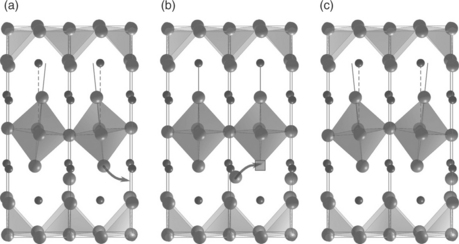
A1.1 Characteristic snapshots of the oxygen interstitialcy diffusion mechanism predicted by MD calculations for the diffusion of Pr2NiO4+δ. (a) An apical oxygen ion from the NiO6 octahedron progresses to an adjacent oxygen interstitial site, (b) the oxygen interstitial moves to the vacant apical site and (c) the final state. Praseodymium ions are represented by small spheres, oxygen by large spheres, the oxygen vacancy by a square. Nickel–oxygen polyhedra are also shown.
Considering oxygen diffusivities, the calculated diffusivities were consistent with experimental values for both La2NiO4 + δ and Pr2NiO4 + δ.31,33,40,44 Interestingly, for Pr2NiO4 + δ, MD calculations indicate that the activation energy for oxygen migration depends strongly upon the degree of hyperstoichiometry – ranging from 0.49 eV (δ = 0.025) to higher values 0.64 eV (δ = 0.20).40 It was proposed that the oxygen diffusivity D at a temperature T can be described by D = [Oi] f exp(− Em/kBT), where [Oi] is the concentration of oxygen interstitials, f is the correlation factor, Em is the energy barrier to migration and kB is Boltzmann’s constant.40 First, there is a rapid diffusivity rise as a function of increasing oxygen interstitial concentration. This is because interstitial ions mediate oxygen diffusion in the interstitialcy mechanism. Beyond δ ~ 0.02, however, the diffusivity levels off. This is due to the increased activation energy for interstitialcy migration because of the presence of other pre-existing neighbouring interstitials, which effectively stiffens the lattice. The stiffening is due to the hindrance of the NiO6 sublattice reorientation, effectively reducing the ability of the octahedra to tilt, which assists the passage of the migrating oxygen ions.
As a second example of the application of MD we will consider ordered GdBaCo2O5 + 8. For this material the oxygen activation energy was calculated to be 0.5 eV (for T = 800–1400 K) in excellent agreement with the experimental value of 0.6 eV obtained by isotopic exchange techniques in the temperature range 600–1000 K.34,45,46 The high-temperature tetragonal phase GdBaCo2O5+δ exhibits a highly anisotropic oxygen diffusion (vacancy mediated) along the a–b plane.45,46 This is also consistent with experimental results.34
In GdBaCo2O5 + δ there is a level of exchange between the Gd with Ba cations. We quantify this with a parameter F = [GdBa]/([GdBa]+[GdGd]), which represents the probability of finding a Gd ion on a Ba site, where [MN] represents the concentration of M ions on an N site. For the fully disordered case there is a 50% probability of either site being occupied by a Gd or Ba ion (i.e., F = 0.5), whereas for the fully ordered case F = 0.
In Plate VII (see colour section between pages 238 and 239) we show the effect of cation disorder upon the oxygen diffusion mechanism for F = 0, 0.1, and 0.5, where the pathways are indicated by contiguous red lines. It is clear that the formation of cation-disordered defects enables migration pathways along the c-axis. That is, an increase of disorder results leads to the reduction of anisotropy of oxygen transport in GdBaCo2O5 + δ. For F = 0.5 there is a drop in the oxygen diffusivity and the mechanism can be considered to be almost isotropic. As the levels of cation disorder are important, experimental conditions such as sample preparation and thermal history can be used to tune the anisotropy of the material.
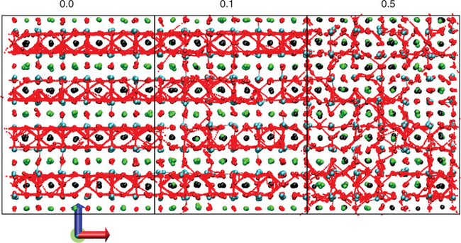
Plate VII The impact of disorder (F > 0) in the Gd/Ba sublattice on the oxygen diffusion mechanism in GdBaCo2O5.5. Black spheres represent Gd cations; green spheres, Ba cations; light blue spheres, Co cations and red spheres, the oxygen anions. The degree of Gd/Ba disorder, F, is indicated at the top, where 0.0 indicates a fully ordered structure and 0.5 indicated complete disorder.
A number of other issues can also be investigated using simulation when selecting RP series materials for SOFC cathodes. For example, Kim et al.36 propose the use of intermediate size rare-earth cations such as samarium to avoid the decrease in the thermal expansion coefficient observed with the smaller rare-earth cations. Simulation can investigate a range of such substitutions and different combinations and suggest optimized composition combinations. Substitution can also be considered for the divalent cation with barium exchanged with strontium in GdBaCo2O5+δ leading to GdBa1 – x SrxCo2O5 + δ, which has an increased oxygen content.37 This increase will in turn affect the transport properties and is presently under investigation but it is not clear how such substitutions might influence the anion activation energy, especially as a function of substitution concentration.
To conclude, MD modelling can provide valuable insight into the oxygen diffusion properties in SOFC cathode materials. In the RP series the composition is key to achieving high oxygen diffusion. Increasing the oxygen hyperstoichiometry (i.e., the oxygen interstitials that mediate diffusion) affects the energetics of oxygen transport but such effect are observed to levels off as the hyperstoichiometry is increased – simulation can help provide an explanation for such phenomena. In GdBaCo2O5+δ and related compounds cation disorder is of critical importance not only for the energetics of diffusion but also for the diffusion mechanism. The more disordered the material, the more isotropic oxygen transport becomes. Again, it is highly useful to gain a mechanistic understanding of such processes in order to develop strategies for further experimental investigation.
A.3.2 Random semiconductor alloys
An area of study where QM-based DFT calculations can be of particular importance is the modelling of semiconductor alloys. For such systems there exist numerous potential models,47,48 which can efficiently describe some aspects of their mechanical properties. Nevertheless, the advent of more powerful computational resources has facilitated the use of DFT, which is able to make more wide ranging property predictions. Here we will mainly focus on binary and ternary group IV alloys (for example Si1 – x – yGexSny) but we will also briefly consider ternary III–V alloys (such as In1 – xGaxAs). These systems are very promising for a number of photovoltaic, nanoelectronic, detector and laser applications.49–61
The Sn-based binary and ternary Si.1 − x – yGexSny random alloys have recently attracted significant attention because, by varying the concentration of the constituent elements, their lattice parameters, mechanical and electronic properties can be tuned. Of particular interest has been the synthesis of Si1 – x – yGexSny alloys with Si content of up to 32% and Sn content of up to 10%.62,63 These can be effectively considered as random alloys as the three elements (Si, Ge and Sn) randomly occupy the available substitutional sites on the underlying diamond lattice. In terms of computational modelling, what makes random alloys qualitatively and quantitatively different compared to ordered alloys is their vast number of different local environments, which in turn can influence the defect processes.64–69
One way to model these alloys is by the construction of a large block of atoms in which the lattice sites will be randomly decorated by the three constituent elements. To achieve, however, a random cell that contains a statistically representative number of all the possible nearest-neighbour (NN) environments, will require many hundreds or even thousands of atoms.
Thereafter, even if one considers the modelling of the interaction of simple NN dopant–defect pairs with respect to their NN environment, it will result in 900 distinct combinations. This is because there are 100 ways of distributing the Si, Ge and Sn atoms at NN atoms around a substitutional dopant (such a As) and a defect (such as a lattice vacancy, V) and there are nine distinct NN AsV pairs.65 For example, the AsSnVSi pair (As atom at a Sn substitutional site, V of a Si atom) is different to an AsGeVSi pair (As atom at a Ge substitutional site, V of a Si atom) and there are nine such combinations.
It becomes apparent that considering so many different configurations in large supercells with DFT becomes computationally overwhelming. A way to make similar issues computationally tractable is the use of specific distributions such as the special quasirandom structures (SQS) developed by Zunger et al.64 The main advantage of the SQS approach is that it mimics the most relevant near-neighbour pair and multisite correlation functions of random alloys with the use of specially designed small-unit-cell periodic structures.65,66 An example of a 32-atom SQS cell for ternary Aa5B0.25C0.25 and A05B0375C0125 alloys is illustrated in Fig. A1.2.
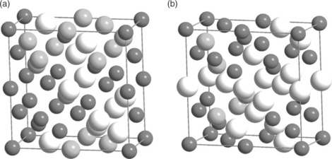
A1.2 32-atom SQSs for (a) A0.5B0.25C0.25 and (b) A0.5B0.375C0.125 alloys (Reference 70) with diamond crystal structure. Dark grey, white and light grey spheres represent A, B and C atoms, respectively.
By expanding this 32-atom cell one can create the larger supercells required for the DFT calculations. For example, by expanding the SQS cell by 1 × 1 × 2 one can generate 64-atom supercells, which can adequately describe the properties of random alloys within the capability of present computational resources.
In a recent computational study (DFT/SQS), a 64-atom supercell of Si0.375Ge0.5Sn0.125 alloy (refer to Fig. A1.2b and expand by 1 × 1 × 2) was used to investigate the AsV pairs.70 This particular system is of interest as AsV pairs may form in quantum cells employing Si1 − x − yGexSny buffer layers.70 For example, in a GaInP/GaAs/Ge quantum well As can penetrate into the Ge layers.71,72 This will affect the properties of Ge as As is a donor species; furthermore, it can diffuse quickly via a vacancy mechanism and can form large AsnVm complexes.73–75 Interestingly, the DFT/SQS approach demonstrated that the NN environment can strongly influence the stability of the AsV pairs in Si0.375Ge0.5Sn0.125.70 An extreme example is the AsSiVSi pair with 2 Si and 1 Sn atoms at NN sites to AsSi, and 2 Ge atoms and a Sn atom at NN sites to the VSi. This pair has a binding energy of − 0.14 eV and it is therefore energetically favourable to form. However, if the Sn NN atom to the VSi is replaced by a Si atom, the binding energy becomes 0.84 eV, which means that the VSi will repel the AsSi atom.70
The importance of the NN environment around vacancies in group IV alloys has also been determined experimentally. For example, positron annihilation investigations indicated that it is energetically favourable for a Ge atom to replace a Si atom at a NN site to a V in Si1 − xGex.76 This experimental result is consistent with previous DFT/SQS calculations in Si1 − xGex.67,76,77
The calculations for Si0.375Ge0.5Sn0.125 reveal that the effect of the secondNN (2NN) environment on the stability of the AsV pair is less important.70 Generally, it is calculated that AsV pairs are less bound in Si0.375Ge0.5Sn0.125 than is Si but more bound than is Ge. Therefore, in layers with compositional differences there might be concentration variations of the AsV pairs and isolated V or As atoms.
Previous DFT/SQS work on binary random alloys A. 1 − xBx, (including Si1 − xGex and Sn1 − xGex) predicted that their lattice parameter deviates from the linear interpolation of the lattice parameter of the constituent elements (i.e., they deviate from Vegard’s law)78 This deviation from linearity as a function of the composition x, Δa(x), is defined65 as
where aB, aA and aAB are the lattice parameters of A, B and A1 − xBx, respectively. Using Equation [A.1] a positive Δa(x) value corresponds to a negative bowing of the lattice parameter. As determined by Kouvetakis et al.,49 the bowing of the lattice parameter is negative for Si. 1 − xGex but positive for Sn1 − xGex alloys, and this has been verified in recent DFT/SQS investigations.67,68
Similar approaches are important in group III–V random alloys. Interestingly, in a recent DFT/SQS study, Murphy et al.69 investigated the relationship between the difference in covalent radii of the constituent group III atoms and the extent of the deviation from Vegard’s law in a range of ternary group III arsenides. Similar systematic investigations can elucidate the structure–property relations of these important systems.
A.4 Future trends
The aim of this appendix was to briefly review important computational modelling techniques and to illustrate their applicability through examples that employed different approaches. Computational modelling techniques are a valuable tool in the study of functional energy materials and this role will become increasingly important in the future with the ever-increasing available computational power. These techniques can calculate properties over an extensive range of compositions relatively quickly at a fraction of the cost of advanced experimental methods. Additionally, they can predict the behaviour of systems where there is very limited or no experimental evidence. Finally, as we have seen in the examples, they are able to identify the atomic-scale mechanisms that underpin technologically significant phenomena (e.g., mass transport). Thus, simulation can not only guide experimentalists to compositions of interest but can also identify novel materials and aid in their design from the atomic scale upwards. This is significant given the current interest in nanosized materials that are characterized by the reduced transport lengths and size-dependent properties, which may not be adequately described by contemporary theory. To conclude, computational modelling techniques in synergy with advanced experimental methods can provide a more complete picture for present and emerging issues in functional energy materials.
A.5 References
1. Stoneham, A.M. Theory of Defects in Solids – Electronic Structure of Defects in Insulators and Semi-Conductors. Oxford University Press; 1985.
2. Leach, A.R. Molecular Modelling – Principles and Applications, 2nd Edition. Pearson Education Ltd, 2001.
3. Nosé, S. Mol. Phys.. 1984; 52:255.
4. Swope, W.C., Andersen, H.C., Berens, P.H., Wilson, K.R. J. Chem. Phys.. 1982; 76:637.
5. Hockney, R.W. Meth. Comput. Phys.. 1970; 9:136.
6. Allen, M.P., Tildesley, D.J. Computer Simulations of Liquids. Oxford Science Publications; 1989.
7. Slater, J. Phys. Rev.. 1931; 37:682.
8. Ewald, P. Ann. derPhysik. 1921; 369:253.
9. Tersoff, J. Phys. Rev. Lett.. 1988; 61:2879.
10. Stillinger, F.H., Weber, T.A. Phys. Rev. B. 1985; 31:5262.
11. Mitchell, P.J., Fincham, D. J. Phys. Condens. Matter. 1993; 5:1031.
12. Schroeder, U. Solid State Commun.. 1966; 4:347–349.
13. Madden, P.A., Wilson, M. Chem. Soc. Rev. 1996; 25:339.
14. Rowley, A.J., Jemmer, P., Wilson, M., Madden, P.A. J. Chem. Phys.. 1998; 108:10209.
15. Daw, M.S., Baskes, M.I. Phys. Rev. B. 1984; 29:6443–6453.
16. Kohn, W., Sham, L.J. Phys. Rev.. 1965; 140:A1133.
17. Becke, A.D. Phys. Rev.. 1988; A38:3098.
18. Becke, A.D. J. Chem. Phys. 1993; 98:5648.
19. Stephens, P.J., Devlin, F.J., Chabalowski, C.F., Frisch, M.J. J. Phys. Chem.. 1994; 98:11623.
20. Becke, A.D. J. Chem. Phys.. 1993; 98:1372.
21. Li, Z., Scheraga, H.A. Proc. Natn. Acad. Sci. USA. 1987; 84:6611.
22. Erman, B., Bahar, I., Jemican, R.L. J. Chem. Phys.. 1997; 107:2046.
23. Zacate, M.O., Grimes, R.W. J. Phys. Chem. Solids. 2002; 63:675.
24. Zacate, M.O., Grimes, R.W. Philos. Mag. A. 2000; 80:797.
25. Kantorovich, L.N., Shluger, A.L., Stoneham, A.M. Phys. Rev. B. 2001; 63:184111.
26. Steele, B.C.H., Heinzel, A. Nature. 2001; 414:345.
27. Fleig, J. Ann. Rev. Mater. Res.. 2003; 33:361.
28. Shao, Z., Haile, S.M., Ahn, J., Ronney, P.D., Zhan, Z., Barnett, S.A. Nature. 2005; 435:3676.
29. Adler, S.B., Lane, J.A., Steele, B.C.H. J. Electrochem. Soc.. 1996; 143:3554.
30. Adler, S.B. Solid State Ionics. 1998; 111:125.
31. Boehm, E., Bassat, J.M., Dordor, P., Mauvy, F., Grenier, J.C., Stevens, Ph. Solid State Ionics. 2005; 176:2717.
32. Burriel, M., Garcia, G., Santiso, J., Kilner, J.A., Chater, R.J., Skinner, S.J. J. Mater. Chem.. 2008; 18:416.
33. Chroneos, A., Parfitt, D., Kilner, J.A., Grimes, R.W. J. Mater. Chem.. 2010; 20:266.
34. Tarancón, A., Skinner, S.J., Chater, R.J., Hernandez-Ramirez, F., Kilner, J.A. J. Mater. Chem.. 2007; 17:3175.
35. Zhu, C.J., Liu, X.M., Yi, C.S., Yan, D., Su, W.H. J. Power Sources. 2008; 185:193.
36. Kim, J.H., Manthiran, A. J. Electrochem. Soc.. 2008; 155:B385.
37. Kim, J.H., Prado, F., Manthiran, A. J. Electrochem. Soc.. 2008; 155:B1023.
38. Mazo, G.N., Savvin, S.N. Solid State Ionics. 2004; 175:371.
39. Rupasov, D., Chroneos, A., Parfitt, D., Kilner, J.A., Grimes, R.W., Ya Istomin, S., Antipov, E.V. Phys. Rev. B. 2009; 79:172102.
40. Parfitt, D., Chroneos, A., Kilner, J.A., Grimes, R.W. Phys. Chem. Chem. Phys.. 2010; 12:6834.
41. Kushima, A., Parfitt, D., Chroneos, A., Yildiz, B., Kilner, J.A., Grimes, R.W. Phys. Chem. Chem. Phys. 2011; 13:2242.
42. Naumovich, E.N., Kharton, V.V. J. Mol. Struct. THEOCHEM. 2010; 946:57.
43. Chroneos, A., Vovk, R.V., Goulatis, I.L., Goulatis, L.I. J. Alloys Compd.. 2010; 494:190.
44. Sayers, R., De Souza, R.A., Kilner, J.A., Skinner, S.J. Solid State Ionics. 2010; 181:386.
45. Tarancón, A., Parfitt, D., Chroneos, A., Kilner, J.A.Connor P., ed. The European Solid Oxide Fuel Cell Forum. Proceedings of 9th European SOFC Forum, 2010:10.93–10.98.
46. Parfitt, D., Chroneos, A., Tarancon, A., Kilner, J.A. J. Mater. Chem.. 2011; 21:2183.
47. Stillinger, F.H., Weber, T.A. Phys. Rev. B. 1985; 31:5262.
48. Tersoff, J. Phys. Rev. B. 1988; 37:6991.
49. Kouvetakis, J., Menendez, J., Chizmeshya, A.V.G. Ann. Rev. Mater. Res.. 2006; 36:497.
50. Roucka, R., Tolle, J., Cook, C., Chizmeshya, A.V.G., Kouvetakis, J., D’Costa, V., Menendez, J., Chen, Z.D. Appl. Phys. Lett. 2005; 86:191912.
51. D’Costa, V.R., Fang, Y.Y., Tolle, J., Kouvetakis, J., Menendez, J. Phys. Rev. Lett. 2009; 102:107403.
52. Sun, G., Cheng, H.H., Menendez, J. Appl. Phys. Lett. 2007; 90:251105.
53. Chizmeshya, A.V.G., Ritter, C., Tolle, J., Cook, C., Menendez, J., Kouvetakis, J. Chem. Mater.. 2006; 18:6266.
54. Wistey, M.A., Fang, Y.Y., Tolle, J., Chizmeshya, A.V.G., Kouvetakis, J. Appl. Phys. Lett. 2007; 90:082108.
55. D’Costa, V.R., Cook, C.S., Birdwell, A.G., Littler, C.L., Canonico, M., Zollner, S., Kouvetakis, J., Menendez, J. Phys. Rev. B. 2006; 73:125207.
56. D’Costa, V.R., Tolle, J., Poweleit, C.D., Kouvetakis, J., Menendez, J. Phys. Rev. B. 2007; 76:035211.
57. Nötzel, R., Temmyo, J., Tamamura, T. Nature. 1994; 369:131.
58. De Caro, L., Giannini, C., Tapfer, L., Schönherr, H.P., Daweritz, L., Ploog, K.H. Solid State Commun.. 1998; 108:599.
59. Zhou, D., Usher, B.F. J. Phys. D: Appl. Phys. 2001; 34:1461.
60. Kunets, V.P., Morgan, T.A., Mazur, Y.I., Dorogan, V.G., Lytvyn, P.M., Ware, M.E., Guzun, D., Shultz, J.L., Salamo, G.J. J. Appl. Phys. 2008; 104:103709.
61. Lin, D.M., Huang, C.C., Chan, Y.J. IEEE Trans. Electron Devices. 2009; 56:2638.
62. Bauer, M., Ritter, C., Crozier, P.A., Ren, J., Menendez, J., Wolf, G., Kouvetakis, J. Appl. Phys. Lett. 2003; 83:2163.
63. Bauer, M.R., Cook, C.S., Aella, P., Tolle, J., Kouvetakis, J., Crozier, P.A., Chizmeshya, A.V.G., Smith, D.J., Zollner, S. Appl. Phys. Lett. 2003; 83:3489.
64. Zunger, A., Wei, S.H., Ferreira, L.G., Bernard, J.E. Phys. Rev. Lett.. 1990; 65:353.
65. Venezuela, P., Dalpian, G.M., da Silva, A.J.R., Fazzio, A. Phys. Rev. B. 2001; 64:193202.
66. Jiang, C., Wolverton, C., Sofo, J., Chen, L.Q., Liu, Z.K. Phys. Rev. B. 2004; 69:214202.
67. Chroneos, A., Bracht, H., Jiang, C., Uberuaga, B.P., Grimes, R.W. Phys. Rev. B. 2008; 78:195201.
68. Chroneos, A., Jiang, C., Grimes, R.W., Schwingenschlögl, U., Bracht, H. Appl. Phys. Lett. 2009; 94:252104.
69. Murphy, S.T., Chroneos, A., Jiang, C., Schwingenschlögl, U., Grimes, R.W. Phys. Rev. B. 2010; 82:073201.
70. Chroneos, A., Jiang, C., Grimes, R.W., Schwingenschlögl, U., Bracht, H. Appl. Phys. Lett. 2009; 95:112101.
71. Barnham, K., Connolly, J., Griffin, P., Haarpaintner, G., Nelson, J., Tsui, E., Zachariou, A., Osborne, J., Button, C., Hill, G., Hopkinson, M., Pate, M., Roberts, J., Foxon, T. J. Appl. Phys. 1996; 80:1201.
72. Rohr, C., Abbott, P., Ballard, I., Connolly, J.P., Barnham, K.W.J., Mazzer, M., Button, C., Nasi, L., Hill, G., Roberts, J.S., Clarke, G., Ginige, R. J. Appl. Phys. 2006; 100:114510.
73. Chroneos, A., Grimes, R.W., Uberuaga, B.P., Brotzmann, S., Bracht, H. Appl. Phys. Lett. 2007; 91:192106.
74. Brotzmann, S., Bracht, H. J. Appl. Phys. 2008; 103:033508.
75. Chroneos, A., Bracht, H., Grimes, R.W., Uberuaga, B.P. Appl. Phys. Lett.. 2008; 92:172103.
76. Sihto, S.L., Slotte, J., Lento, J., Saarinen, K., Monakhov, E.V., Kuznetsov, A.Yu., Svensson, B.G. Phys. Rev. B. 2003; 68:115307.
77. Venezuela, P., Dalpian, G.M., da Silva, A.J.R., Fazzio, A. Phys. Rev. B. 2002; 65:193306.