2
COMBINATORIAL LOGIC

In the 1967 Star Trek episode “The City on the Edge of Forever,” Mr. Spock says, “I am endeavoring, ma’am, to construct a mnemonic memory circuit using stone knives and bearskins.” Like Mr. Spock, people have come up with all sorts of ingenious ways to build computing devices using the resources available to them. Few fundamental technologies were invented explicitly for computing; most were invented for other purposes and then adapted for computing. This chapter covers some of this evolution, leading up to the convenient but fairly recent innovation of electricity.

In Chapter 1, you learned that modern computers use binary containers called bits for their internal language. You may wonder why computers use bits when decimal numbers work fine for people. In this chapter, we’ll start by looking at some early computing devices that didn’t use bits to learn why bits are the right choice for the technology available today. Bits aren’t found naturally in a useful form for computing, so we’ll talk about what’s needed to make them. We’ll work through some older, simpler technologies like relays and vacuum tubes, then compare them to the modern implementation of bits in hardware using electricity and integrated circuits.

The discussion of bits in Chapter 1 was pretty abstract. Here we’ll be getting down to the nitty-gritty. Physical devices, including those that operate on bits, are called hardware. We’ll talk about hardware that implements combinatorial logic, another name for the Boolean algebra discussed in Chapter 1. And just as you did in that chapter, here you’ll learn about the simple building blocks first and then we’ll combine them to yield more complex functionality.

The Case for Digital Computers

Let’s begin by looking at some gear-based mechanical computing devices that predate the modern era. When two gears are meshed together, the ratio of the number of teeth on each gear determines their relative speed, making them useful for multiplication, division, and other calculations. One gear-based mechanical device is the Antikythera mechanism, the oldest known example of a computer, found off a Greek island and dating back to around 100 BCE. It performed astronomical calculations whereby the user entered a date by turning a dial and then turned a crank to get the positions of the sun and the moon on that date. Another example is World War II–era artillery fire control computers, which performed trigonometry and calculus using lots of strangely shaped gears with a complex design that made them works of art as well.

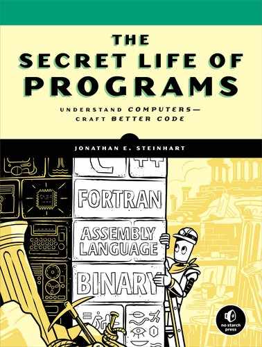
An example of a mechanical computer that doesn’t use gears is the slide rule, invented by English minister and mathematician William Oughtred (1574–1660). It’s a clever application of logarithms that were discovered by Scottish physicist, astronomer, and mathematician John Napier (1550–1617). The basic function of a slide rule is to perform multiplication by exploiting the fact that log(x × y) = log(x) + log(y).

A slide rule has fixed and moving scales marked in logarithms. It computes the product of two numbers by lining up the fixed x scale with the moving y scale, as shown in Figure 2-1.

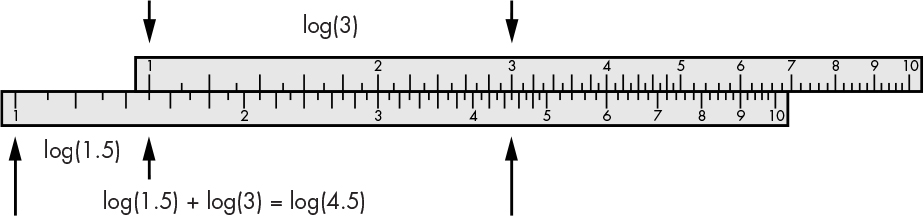
Figure 2-1: Slide rule addition

Considered by many to be the first mass-produced computing device, the slide rule is a great example of how people solved a problem using the technology available to them at the time. Today, airplane pilots still use a circular version of the slide rule called a flight computer that performs navigation-related calculations as a backup device.

Counting is a historically important application of computing devices. Because of our limited supply of fingers—and the fact that we need them for other things—notched bones and sticks called tally sticks were used as computing aids as early as 18,000 BCE. There is even a theory that the Egyptian Eye of Horus was used to represent binary fractions.

English polymath Charles Babbage (1791–1871) convinced the British government to fund the construction of a complex decimal mechanical calculator called a difference engine, which was originally conceived by Hessian army engineer Johann Helfrich von Müller (1746–1830). Popularized by the William Gibson and Bruce Sterling novel named after it, the difference engine was ahead of its time because the metalworking technologies of the period were not up to the task of making parts with the required precision.

Simple decimal mechanical calculators could be built, however, as they didn’t require the same level of metalworking sophistication. For example, adding machines that could add decimal numbers were created in the mid-1600s for bookkeeping and accounting. Many different models were mass-produced, and later versions of adding machines replaced hand-operated levers with electric motors that made them easier to operate. In fact, the iconic old-fashioned cash register was an adding machine combined with a money drawer.

All of these historical examples fall into two distinct categories, as we’ll discuss next.

The Difference Between Analog and Digital

There’s an important difference between devices such as the slide rule versus tally sticks or adding machines. Figure 2-2 illustrates one of the slide rule scales from Figure 2-1 compared to a set of numbered fingers.

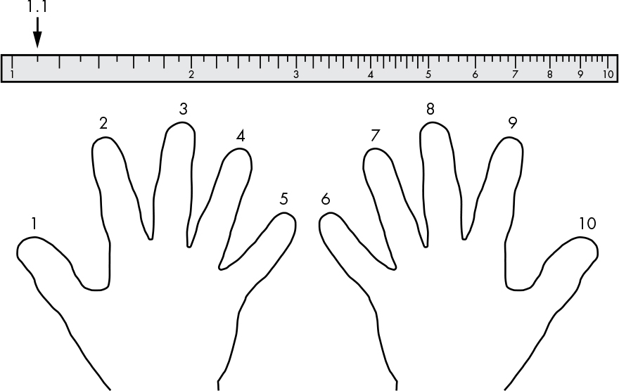
Figure 2-2: Continuous and discrete measures

Both the slide rule scale and the fingers go from 1 to 10. We can represent values such as 1.1 on the scale, which is pretty handy, but we can’t do that using fingers without some fancy prestidigitation (sleight of hand or maybe doing the hand jive). That’s because the scale is what mathematicians call continuous, meaning that it can represent real numbers. The fingers, on the other hand, are what mathematicians call discrete and can only represent integers. There are no values between integers. They jump from one whole number value to another, like our fingers.

When we’re talking about electronics, we use the word analog to mean continuous and digital to mean discrete (it’s easy to remember that fingers are digital because the Latin word for finger is digitus). You’ve probably heard the terms analog and digital before. You’ve been learning to program using digital computers, of course, but you may not have been aware that analog computers such as slide rules also exist.

On one hand, analog appears to be the better choice for computing because it can represent real numbers. But there are problems with precision. For example, we can pick out the number 1.1 on the slide rule scale in Figure 2-2 because that part of the scale is spacious and there’s a mark for it. But it’s much harder to find 9.1 because that part of the scale is more crowded and the number is somewhere between the tick marks for 9.0 and 9.2. The difference between 9.1 and 9.105 would be difficult to discern even with a microscope.

Of course, we could make the scales larger. For example, we could get a lot more accurate if the scale were the length of a football field. But it would be hard to make a portable computer with 120-yard-long scales, not to mention the huge amount of energy it would take to manipulate such large objects. We want computers that are small, fast, and low in power consumption. We’ll learn another reason why size is important in the next section.

Why Size Matters in Hardware

Imagine you have to drive your kids to and from school, which is 10 miles away, at an average speed of 40 miles per hour. The combination of distance and speed means that only two round trips per hour are possible. You can’t complete the trip more quickly without either driving faster or moving closer to school.

Modern computers drive electrons around instead of kids. Electricity travels at the speed of light, which is about 300 million meters per second (except in the US, where it goes about a billion feet per second). Because we haven’t yet discovered a way around this physical limitation, the only way we can minimize travel time in computers is to have the parts close together.

Computers today can have clock speeds around 4 GHz, which means they can do four billion things per second. Electricity only travels about 75 millimeters in a four-billionth of a second.

Figure 2-3 shows a typical CPU that measures about 18 millimeters on each side. There’s just enough time to make two complete round trips across this CPU in four-billionths of a second. It follows that making things small permits higher performance.

Figure 2-3: CPU photomicrograph (Courtesy of Intel Corporation)

Also, just like driving kids to and from school, it takes energy to travel, and coffee alone is insufficient. Making things small reduces the amount of travel needed, which reduces the amount of energy needed. That translates into lower power consumption and less heat generation, which keeps your phone from burning a hole in your pocket. This is one of the reasons why the history of computing devices has been characterized by efforts to make hardware smaller. But making things very small introduces other problems.

Digital Makes for More Stable Devices

Although making things small allows for speed and efficiency, it’s pretty easy to interfere with things that are very small. German physicist Werner Heisenberg (1901–1976) was absolutely certain about that.

Picture a glass measuring cup with lines marked for 1 through 10 ounces. If you put some water in the cup and hold it up, it may be hard to tell how many ounces are in the cup because your hand shakes a little. Now imagine that the measuring cup was a billion times smaller. Nobody would be able to hold it still enough to get an accurate reading. In fact, even if you put that tiny cup on a table, it still wouldn’t work because at that size, atomic motion would keep it from holding still. At very small scales, the universe is a noisy place.

Both the measuring cup and the slide rule are analog (continuous) devices that don’t take much jiggling to produce incorrect readings. Disturbances like stray cosmic radiation are enough to make waves in microscopic measuring cups, but they’re less likely to affect discrete devices such as fingers, tally sticks, or mechanical calculators. That’s because discrete devices employ decision criteria. There are no “between” values when you’re counting on your fingers. We could modify a slide rule to include decision criteria by adding detents (some sort of mechanical sticky spots) at the integer positions. But as soon as we do that, we’ve made it a discrete device and eliminated its ability to represent real numbers. In effect, decision criteria prevent certain ranges of values from being represented. Mathematically, this is similar to rounding numbers to the nearest integer.

So far, we’ve talked about interference as if it comes from outside, so you might think we could minimize it by using some sort of shielding. After all, lead protected Superman from kryptonite. But there is another, more insidious source of interference. Electricity affects things at a distance, just like gravity—which is good, or we wouldn’t have radio. But that also means that a signal traveling down a wire on a chip can affect signals on other wires, especially when they’re so close together. The wires on a modern computer chip are a few nanometers (10^–9 meters) apart. For comparison, a human hair is about 100,000 nanometers in diameter. This interference is a bit like the wind you feel when two cars pass each other on the road. Because there’s no simple way to protect against this crosstalk effect, using digital circuitry that has higher noise immunity from the decision criteria is essential. We could, of course, decrease the impact of interference by making things bigger so that wires are farther apart, but that would run counter to our other goals. The extra energy it takes to jump over the hurdle of a decision criterion gives us a degree of immunity from the noise that we don’t get by using continuous devices.

In fact, the stability that comes from using decision criteria is the primary reason we build digital (discrete) computers. But, as you may have noticed, the world is an analog (continuous) place, as long as we stay away from things that are so small that quantum physics applies. In the next section, you’ll learn how we manipulate the analog world to get the digital behavior necessary for building stable computing devices.

Digital in an Analog World

A lot of engineering involves clever applications of naturally occurring transfer functions discovered by scientists. These are just like the functions you learn about in math class, except they represent phenomena in the real world. For example, Figure 2-4 shows a graph of the transfer function for a digital camera sensor (or the film in an old-style analog camera, for that matter).

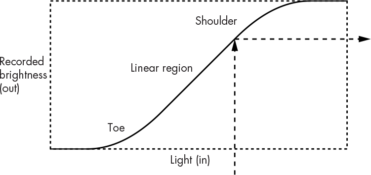
Figure 2-4: Camera sensor or film transfer function

The x-axis shows the amount of light coming in (input), and the y-axis represents the amount of recorded brightness, or the light registered by the sensor (output). The curve represents the relationship between them.

Let’s play transfer function pool by bouncing an input ball off of the curve to get an output. You can see that the transfer function produces different values of recorded brightness for different values of light. Notice that the curve isn’t a straight line. If too much of the light hits the shoulder of the curve, then the image will be overexposed, since the recorded brightness values will be closer together than in the actual scene. Likewise, if we hit the toe of the curve, the shot is going to be underexposed. The goal (unless you’re trying for a special effect) is to adjust your exposure to hit the linear region, which will yield the most faithful representation of reality.

Engineers have developed all manner of tricks to take advantage of transfer functions, such as adjusting the shutter speed and aperture on a camera so that the light hits the linear region. Amplifier circuits, such as those that drive the speakers or earbuds in your music player, are another example.

Figure 2-5 shows the effect that changing the volume has on an amplifier transfer function.

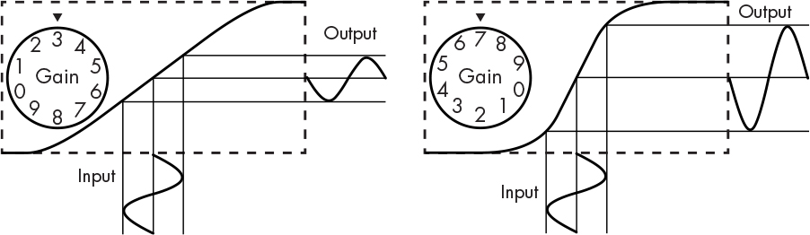
Figure 2-5: Effect of gain on amplifier transfer function

The volume control adjusts the gain, or steepness of the curve. As you can see, the higher the gain, the steeper the curve and the louder the output. But what if we have one of those special amplifiers from the 1984 movie This Is Spinal Tap on which the gain can be cranked up to 11? Then the signal is no longer confined to the linear region. This results in distortion because the output is no longer a faithful reproduction of the input, which makes it sound bad. You can see in Figure 2-6 that the output doesn’t look like the input because the input extends outside the linear region of the transfer function.

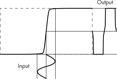
Figure 2-6: Amplifier clipping

A small change in the input causes a jump in the output at the steep part of the curve. It’s like jumping from one finger to another—the sought-after decision criterion, called a threshold. This distortion is a useful phenomenon because the output values fall on one side of the threshold or the other; it’s difficult to hit those in between. This partitions the continuous space into discrete regions, which is what we want for stability and noise immunity—the ability to function in the presence of interference. You can think of analog as aiming for a big linear region and digital as wanting a small one.

You may have intuitively discovered this phenomenon while playing on a seesaw as a child (if you had the good fortune to grow up in an era before educational playground equipment was deemed dangerous, that is). It’s much more stable to be in the toe region (all the way down) or the shoulder region (all the way up) than it is to try to balance somewhere in between.

Why Bits Are Used Instead of Digits

We’ve talked about why digital technology is a better choice for computers than analog. But why do computers use bits instead of digits? After all, people use digits, and we’re really good at counting to 10 because we have 10 fingers.

The obvious reason is that computers don’t have fingers. That would be creepy. On one hand, counting on your fingers may be intuitive, but it’s not a very efficient use of your fingers because you use one finger per digit. On the other hand, if you use each finger to represent a value as you did with bits, you can count to more than 1,000. This is not a new idea; in fact, the Chinese used 6-bit numbers to reference hexagrams in the I Ching as early as 9 BCE. Using bits instead of fingers improves efficiency by a factor of more than 100. Even using groups of four fingers to represent decimal numbers using the binary-coded decimal (BCD) representation we saw in Chapter 1 beats our normal counting method in the efficiency department.

Another reason why bits are better than digits for hardware is that with digits, there’s no simple way to tweak a transfer function to get 10 distinct thresholds. We could build hardware that implements the left side of Figure 2-7, but it would be much more complicated and expensive than 10 copies of the one that implements the right side of the figure.

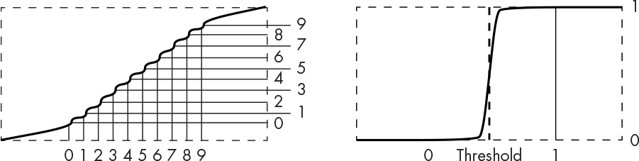
Figure 2-7: Decimal versus binary thresholds

Of course, if we could build 10 thresholds in the same space as one, we’d do that. But, as we’ve seen, we’d be better off with 10 bits instead of one digit. This is how modern hardware works. We take advantage of the transfer function’s toe and shoulder regions, called cutoff and saturation, respectively, in electrical engineering language. There’s plenty of wiggle room; getting the wrong output would take a lot of interference. The transfer function curve is so steep that the output snaps from one value to another.

A Short Primer on Electricity

Modern computers function by manipulating electricity. Electricity makes computers faster and easier to build than other current technologies would. This section will help you learn enough about electricity that you can understand how it’s used in computer hardware.

Using Plumbing to Understand Electricity

Electricity is invisible, which makes it hard to visualize, so let’s imagine that it’s water. Electricity comes from an energy source such as a battery just like water comes from a tank. Batteries run out of energy and need recharging, just like water tanks go dry and need refilling. The sun is the only major source of energy we have; in the case of water, heat from the sun causes evaporation, which turns into rain that refills the tank.

Let’s start with a simple water valve, something like Figure 2-8.

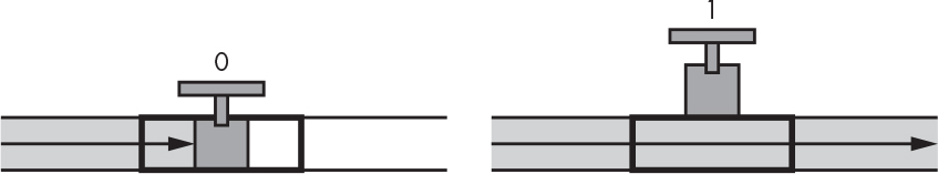
Figure 2-8: A water valve

As you can see, there’s a handle that opens and closes the valve. Figure 2-9 shows a real-life gate valve, which gets its name after the gate that is opened and closed by the handle. Water can get through when the valve is open. We’ll make believe that 0 means closed and 1 means open.

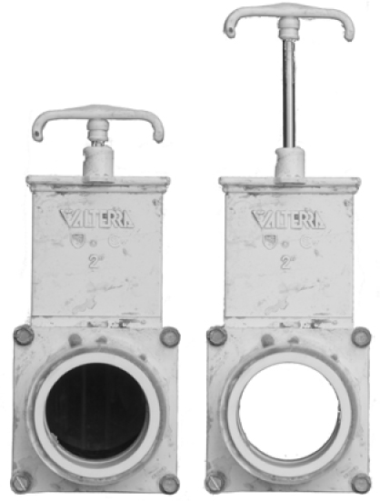
Figure 2-9: Closed and open gate valve

We can use two valves and some pipe to illustrate the AND operation, as shown in Figure 2-10.

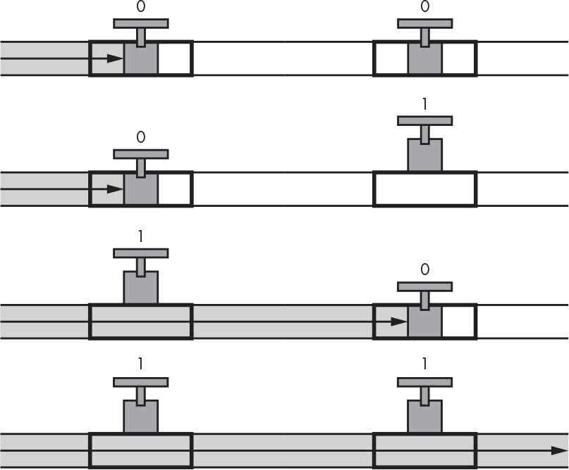
Figure 2-10: Plumbing for the AND operation

As you can see, water flows only when both valves are open, or equal to 1, which as you learned in Chapter 1 is the definition of the AND operation. When the output of one valve is hooked to the input of another, as in Figure 2-10, it’s called a series connection, which implements the AND operation. A parallel connection, as shown in Figure 2-11, results from connecting the inputs of valves and the outputs of valves together, which implements the OR operation.

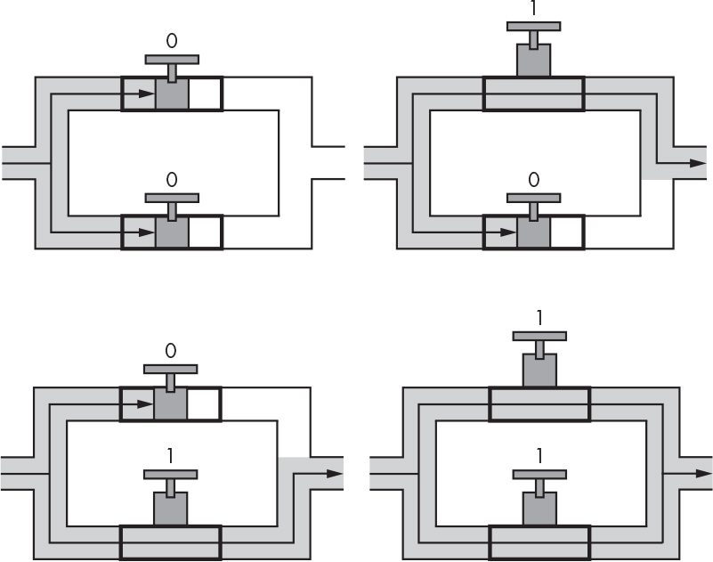
Figure 2-11: Plumbing for the OR operation

Just as it takes time for electricity to make its way across a computer chip, it takes time for water to flow or propagate through a pipe. You’ve probably experienced this when waiting for the water temperature to change in the shower after you’ve turned the knobs. This effect is called propagation delay, and we’ll talk more about it soon. The delay is not a constant; with water, the temperature causes the pipes to expand or contract, which changes the flow rate and thus the delay time.

Electricity travels through a wire like water travels through a pipe. It’s a flow of electrons. There are two parts to a piece of wire: the metal inside, like the space inside a pipe, is the conductor, and the covering on the outside, like the water pipe itself, is the insulator. The flow can be turned on and off with valves. In the world of electricity, valves are called switches. They’re so similar that a mostly obsolete device called a vacuum tube was also known as a thermionic valve.

Water doesn’t just trickle passively through plumbing pipes; it’s pushed by pressure, which can vary in strength. The electrical equivalent of water pressure is voltage, measured in volts (V), named after Italian physicist Alessandro Volta (1745–1827). The amount of flow is called the current (I), and that’s measured in amperes, named after French mathematician André-Marie Ampère (1775–1836).

Water can course through wide pipes or narrow ones, but the narrower the pipe, the more that resistance limits the amount of water that can flow through. Even if you have a lot of voltage (water pressure), you can’t get very much current (flow) if there’s a lot of resistance from using too narrow a conductor (pipe). Resistance (R) is measured in ohms (Ω), named after German mathematician and physicist Georg Simon Ohm (1789–1854).

These three variables—voltage, current, and resistance—are all related by Ohm’s law, which says I = V/R, read as “current equals voltage divided by resistance (ohms).” So, as with water pipes, more resistance means less current. Resistance also turns electricity into heat, which is how everything from toasters to electric blankets works. Figure 2-12 illustrates how resistance makes it harder for voltage to push current.

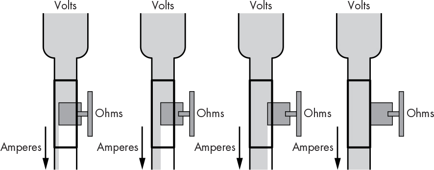
Figure 2-12: Ohm’s law

An easy way to understand Ohm’s law is to suck a milkshake through a straw.

Electrical Switches

Making a switch (valve) for electricity is just a matter of inserting or removing an insulator from between conductors. Think of manually operated light switches. They contain two pieces of metal that either touch or are pushed apart by the handle that operates the switch. It turns out that air is a pretty good insulator; electricity can’t flow if the two pieces of metal aren’t touching. (Notice I said air is a “pretty good” insulator; at a high enough voltage, air ionizes and turns into a conductor. Think lightning.)

The plumbing system in a building can be shown on a blueprint. Electrical systems called circuits are documented using schematic diagrams, which use symbols for each of the components. Figure 2-13 shows the symbol for a simple switch.

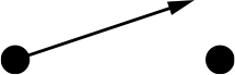
Figure 2-13: Single-pole, single-throw switch schematic

This kind of switch is like a drawbridge: electricity (cars) can’t get from one side to the other when the arrow on the diagram (the bridge) is up. This is easy to see on the old-fashioned knife switches, shown in Figure 2-14 and often featured in cheesy science fiction movies. Knife switches are still used for things like electrical disconnect boxes, but these days they’re usually hidden inside protective containers to make it harder for you to fry yourself.

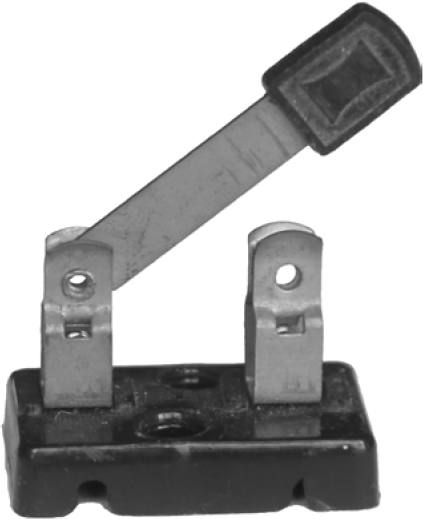
Figure 2-14: Single-pole, single-throw knife switch

Figures 2-13 and 2-14 both show single-pole, single-throw (SPST) switches. A pole is the number of switches connected together that move together. Our water valves in the preceding section were single pole; we could make a double-pole valve by welding a bar between the handles on a pair of valves so that they both move together when you move the bar. Switches and valves can have any number of poles. Single-throw means that there’s only one point of contact: something can be either turned on or off, but not one thing off and another on at the same time. To do that, we’d need a single-pole, double-throw (SPDT) device. Figure 2-15 shows the symbol for such a beast.

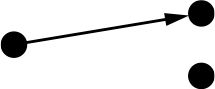
Figure 2-15: SPDT switch schematic

This is like a railroad switch that directs a train onto one track or another, or a pipe that splits into two pipes, as shown in Figure 2-16.

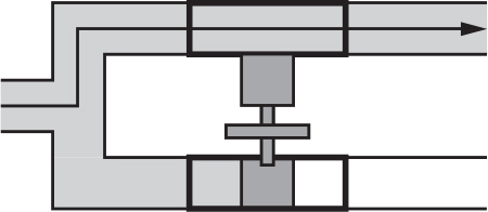
Figure 2-16: SPDT water valve

As you can see, when the handle is pushed down, water flows through the top valve. Water would flow through the bottom valve if the handle were pushed up.

Switch terminology can be extended to describe any number of poles and throws. For example, a double-pole, double-throw (DPDT) switch would be drawn as shown in Figure 2-17, with the dashed line indicating that the poles are ganged, meaning they move together.

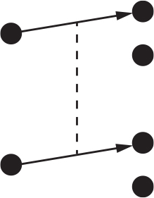
Figure 2-17: DPDT switch schematic

Figure 2-18 shows what a DPDT knife switch looks like in real life.

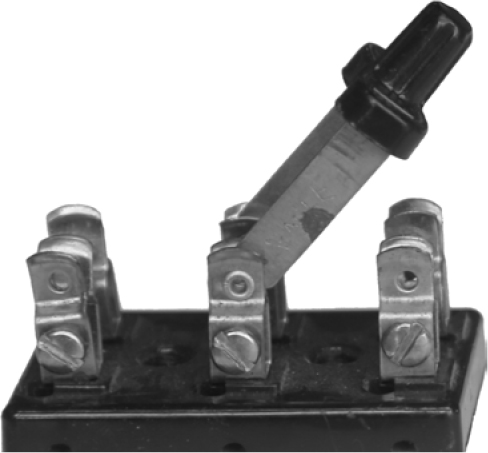
Figure 2-18: DPDT knife switch

I left out a few details about our waterworks earlier: the system won’t work unless the water has somewhere to go. Water can’t go in if the drain is clogged. And there has to be some way to get the water from the drain back to the water tank, or the system will run dry.

Electrical systems are similar. Electricity from the energy source passes through the components and returns to the source. That’s why it’s called an electrical circuit. Or think about it like this: a person running track has to make it back to the starting line in order to do another lap.

Look at the simple electrical circuit in Figure 2-19. It introduces two new symbols, one for a voltage source (on the left) and one for a light bulb (on the right). If you built such a circuit, you could turn the light on and off using the switch.

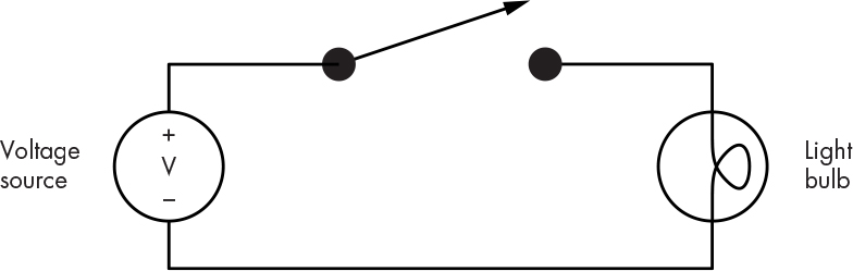
Figure 2-19: A simple electrical circuit

Electricity can’t flow when the switch is open. When the switch is closed, current flows from the voltage source through the switch, through the light bulb, and back to the voltage source. Series and parallel switch arrangements work just like their water valve counterparts.

Now you’ve learned a little about electricity and some basic circuit elements. Although they can be used to implement some simple logic functionality, they’re not powerful enough by themselves to do much else. In the next section, you’ll learn about an additional device that made early electrically powered computers possible.

Building Hardware for Bits

Now that you’ve seen why we use bits for hardware, you’re ready to learn how they’re built. Diving straight into modern-day electronic implementation technologies can be daunting, so instead I’ll build up the discussion from other historical technologies that are easier to understand. Although some of these examples aren’t used in today’s computers, you may still encounter them in systems that work alongside computers, so they’re worth knowing about.

Relays

Electricity was used to power computers long before the invention of electronics. There’s a convenient relationship between electricity and magnetism, discovered by Danish physicist Hans Christian Ørsted (1777–1851) in 1820. If you coil up a bunch of wire and run some electricity through it, it becomes an electromagnet. Electromagnets can be turned on and off and can be used to move things. They can also be used to control water valves, which is how most automatic sprinkler systems work. There are clever ways to make motors using electromagnetism. And waving a magnet around a coil of wire produces electricity, which is how a generator works; that’s how we get most of our electricity, in fact. Just in case you’re inclined to play with these things, turning off the electricity to an electromagnet is equivalent to waving a magnet near the coil very fast. It can be a very shocking experience, but this effect, called back-EMF, is handy; it’s how a car ignition coil makes the spark for the spark plugs. It’s also how electric fences work.

A relay is a device that uses an electromagnet to move a switch. Figure 2-20 shows the symbol for a single-pole, double-throw relay, which you can see looks a lot like the symbol for a switch grafted to a coil.

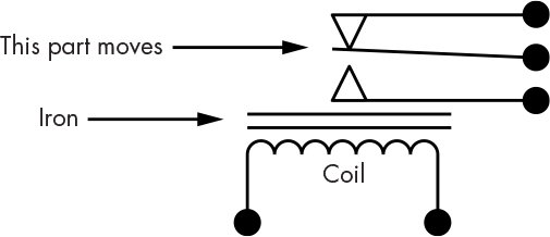
Figure 2-20: SPDT relay schematic

Figure 2-21 shows a real-life example of a single-pole, single-throw relay. The switch part is open when there is no power on the coil, so it’s called a normally open relay. It would be a normally closed relay if the switch were closed without power.

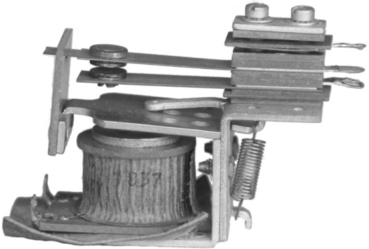
Figure 2-21: Normally open SPST relay

The connections on the bottom go to the coil of wire; the rest looks pretty much like a variation on a switch. The contact in the middle moves depending on whether or not the coil is energized. We can implement logic functions using relays, as shown in Figure 2-22.

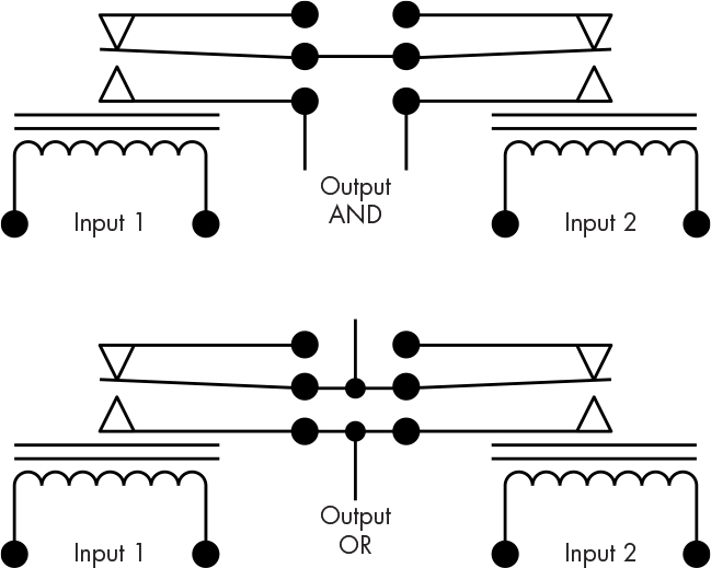
Figure 2-22: Relay circuits for AND and OR functions

On the top of Figure 2-22, you can see that the two output wires are connected together only if both relays are activated, which is our definition of the AND function. Likewise, on the bottom, the wires are connected together if either relay is activated, which is the OR function. Notice the small black dots in this figure. These indicate connections between wires in schematics; wires that cross without a dot aren’t connected.

Relays allow us to do things that are impossible with switches. For example, we can build inverters, which implement the NOT function, without which our Boolean algebra options are very limited. We could use the output from the AND circuit on the top to drive one of the inputs on the OR circuit on the bottom. It’s this ability to make switches control other switches that lets us build the complex logic needed for computers.

People have done amazing things with relays. For example, there is a single-pole, 10-throw stepper relay that has two coils. One coil moves the contact to the next position every time it’s energized, and the other resets the relay by moving the contact back to the first position. Huge buildings full of stepper relays used to count out the digits of telephone numbers as they were dialed to connect calls. Telephone exchanges were very noisy places. Stepper relays are also what give old pinball machines their charm.

Another interesting fact about relays is that the transfer function threshold is vertical; no matter how slowly you increase the voltage on the coil, the switch always snaps from one position to the other. This mystified me as a kid; it was only when studying Lagrange-Hamilton equations as a junior in college that I learned that the value of the transfer function is undefined at the threshold, which causes the snap.

The big problems with relays are that they’re slow, take a lot of electricity, and stop working if dirt (or bugs) get onto the switch contacts. In fact, the term bug was popularized by American computer scientist Grace Hopper in 1947 when an error in the Harvard Mark II computer was traced to a moth trapped in a relay. Another interesting problem comes from using the switch contacts to control other relays. Remember that suddenly turning off the power to a coil generates very high voltage for an instant and that air becomes conductive at high voltages. This phenomenon often results in sparks across the switch contacts, which makes them wear out. Because of these drawbacks, people began looking for something that would do the same work as relays but without moving parts.

Vacuum Tubes

British physicist and electrical engineer Sir John Ambrose Fleming (1849–1945) invented the vacuum tube. He based it on a principle called thermionic emission, which says that if you heat something up enough, the electrons want to jump off. Vacuum tubes have a heater that heats a cathode, which acts like a pitcher in baseball. In a vacuum, electrons (baseballs) flow from the cathode to the anode (catcher). Some examples of vacuum tubes are shown in Figure 2-23.

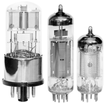
Figure 2-23: Vacuum tubes

Electrons have some properties in common with magnets, including the one where opposite charges attract and like charges repel. A vacuum tube can contain an additional “batter” element, called a grid, that can repel the electrons coming from the cathode to prevent them from getting to the anode. A vacuum tube that contains three elements (cathode, grid, and anode) is called a triode. Figure 2-24 shows the schematic symbol for a triode.

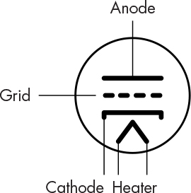
Figure 2-24: Triode schematic

Here, the heater heats up the cathode, making electrons jump off. They land on the anode unless the grid swats them back. You can think of the grid, then, as the handle on a switch.

The advantage of vacuum tubes is that they have no moving parts and are therefore much faster than relays. Disadvantages are that they get very hot and are fragile, just like light bulbs. The heaters burn out like the filaments in light bulbs. But vacuum tubes were still an improvement over relays and allowed the construction of faster and more reliable computers.

Transistors

These days transistors rule. A contraction of transfer resistor, a transistor is similar to a vacuum tube but uses a special type of material, called a semiconductor, that can change between being a conductor and being an insulator. In fact, this property is just what’s needed to make valves for electricity that require no heater and have no moving parts. But, of course, transistors aren’t perfect. We can make them really, really small, which is good, but skinny conductors have more resistance, which generates heat. Getting rid of the heat in a transistor is a real problem, because semiconductors melt easily.

You don’t need to know everything about the guts of transistors. The important thing to know is that a transistor is made on a substrate, or slab, of some semiconducting material, usually silicon. Unlike other technologies such as gears, valves, relays, and vacuum tubes, transistors aren’t individually manufactured objects. They’re made through a process called photolithography, which involves projecting a picture of a transistor onto a silicon wafer and developing it. This process is suitable for mass production because large numbers of transistors can be projected onto a single silicon wafer substrate, developed, and then sliced up into individual components.

There are many different types of transistors, but the two main types are the bipolar junction transistor (BJT) and the field effect transistor (FET). The manufacturing process involves doping, which infuses the substrate material with nasty chemicals like arsenic to change its characteristics. Doping creates regions of p and n type material. Transistor construction involves making p and n sandwiches. Figure 2-25 shows the schematic symbols that are used for some transistor types.

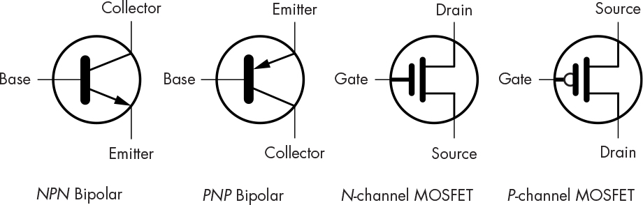
Figure 2-25: Transistor schematic symbols

The terms NPN, PNP, N-channel, and P-channel refer to the sandwich construction. You can think of the transistor as a valve or switch; the gate (or base) is the handle, and electricity flows from the top to the bottom when the handle is raised, similar to how the coil in a relay moves the contacts. But unlike the switches and valves we’ve seen so far, electricity can flow only in one direction with bipolar transistors.

You can see that there’s a gap between the gate and the rest of the transistor in the symbols for the FETs. This gap symbolizes that FETs work using static electricity; it’s like using static cling to move a switch.

The metal-oxide semiconductor field effect transistor, or MOSFET, is a variation on the FET that’s very commonly used in modern computer chips because of its low power consumption. The N-channel and P-channel variants are often used in complementary pairs, which is where the term CMOS (complementary metal oxide semiconductor) originates.

Integrated Circuits

Transistors enabled smaller, faster, and more reliable logic circuitry that took less power. But building even a simple circuit, such as the one that implemented the AND function, still took a lot of components.

This changed in 1958, when Jack Kilby (1923–2005), an American electrical engineer, and Robert Noyce (1927–1990), an American mathematician, physicist, and cofounder of both Fairchild Semiconductor and Intel, invented the integrated circuit. With integrated circuits, complicated systems could be built for about the same cost as building a single transistor. Integrated circuits came to be called chips because of how they look.

As you’ve seen, many of the same types of circuits can be built using relays, vacuum tubes, transistors, or integrated circuits. And with each new technology, these circuits became smaller, cheaper, and more power-efficient. The next section talks about integrated circuits designed for combinatorial logic.

Logic Gates

In the mid-1960s, Jack Kilby’s employer, Texas Instruments, introduced the 5400 and 7400 families of integrated circuits. These chips contained ready-made circuits that performed logic operations. These particular circuits, called logic gates, or simply gates, are hardware implementations of Boolean functions we call combinatorial logic. Texas Instruments sold gazillions of these. They’re still available today.

Logic gates were a huge boon for hardware designers: they no longer had to design everything from scratch and could build complicated logic circuits with the same ease as complicated plumbing. Just like plumbers can find bins of pipe tees, elbows, and unions in a hardware store, logic designers could find “bins” of AND gates, OR gates, XOR gates, and inverters (things that do the NOT operation). Figure 2-26 shows the symbols for these gates.

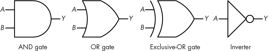
Figure 2-26: Gate schematics

As you would expect, the Y output of the AND gate is true if both the A and B inputs are true. (You can get the operation of the other gates from the truth tables shown back in Figure 1-1.)

The key part of the symbol for an inverter in Figure 2-26 is the ○ (circle), not the triangle it’s attached to. A triangle without the circle is called a buffer, and it just passes its input to the output. The inverter symbol is pretty much used only where an inverter isn’t being used in combination with anything else.

It’s not efficient to build AND and OR gates using the transistor-transistor logic (TTL) technology of the 5400 and 7400 series parts, because the output from a simple gate circuit is naturally inverted, so it takes an inverter to make it come out right side up. This would make them more expensive, slower, and more power-hungry. So, the basic gates were NAND (not and) and NOR (not or), which use the inverting circle and look like Figure 2-27.

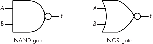
Figure 2-27: NAND and NOR gates

Fortunately, this extra inversion doesn’t affect our ability to design logic circuits because we have De Morgan’s law. Figure 2-28 applies De Morgan’s law to show that a NAND gate is equivalent to an OR gate with inverted inputs.

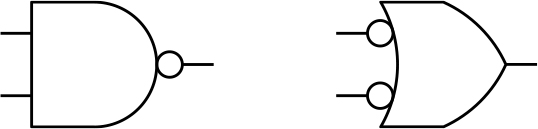
Figure 2-28: Redrawing a NAND gate using De Morgan’s law

All the gates we’ve seen so far have had two inputs, not counting the inverter, but in fact gates can have more than two inputs. For example, a three-input AND gate would have an output of true if each of the three inputs was true. Now that you know how gates work, let’s look at some of the complications that arise when using them.

Improving Noise Immunity with Hysteresis

You saw earlier that we get better noise immunity using digital (discrete) devices because of the decision criteria. But there are situations where that’s not enough. It’s easy to assume that logic signals transition instantaneously from 0 to 1 and vice versa. That’s a good assumption most of the time, especially when we’re connecting gates to each other. But many real-world signals change more slowly.

Let’s see what happens when we have a slowly changing signal. Figure 2-29 shows two signals that ramp slowly from 0 to 1.

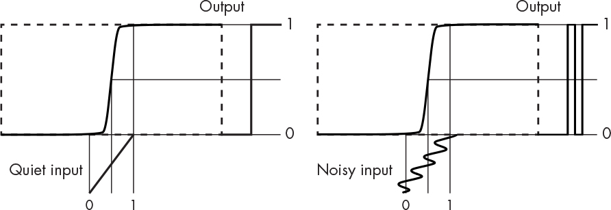
Figure 2-29: Noise glitch

The input on the left is quiet and has no noise, but there’s some noise on the signal on the right. You can see that the noisy signal causes a glitch in the output because the noise makes the signal cross the threshold more than once.

We can get around this using hysteresis, in which the decision criterion is affected by history. As you can see in Figure 2-30, the transfer function is not symmetrical; in effect, there are different transfer functions for rising signals (those going from 0 to 1) and falling signals (those going from 1 to 0) as indicated by the arrows. When the output is 0, the curve on the right is applied, and vice versa.

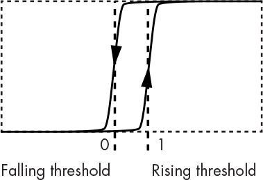
Figure 2-30: Hysteresis transfer function

This gives us two different thresholds: one for rising signals and one for falling signals. This means that when a signal crosses one of the thresholds, it has a lot farther to go before crossing the other, and that translates into higher noise immunity.

Gates that include hysteresis are available. They’re called Schmitt triggers after the American scientist Otto H. Schmitt (1913–1998), who invented the circuit. Because they’re more complicated and expensive than normal gates, they’re used only where they’re really needed. Their schematic symbol depicts the addition of hysteresis, as shown for the inverter in Figure 2-31.

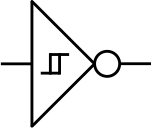
Figure 2-31: Schmitt trigger gate schematic symbol

Differential Signaling

Sometimes there’s so much noise that even hysteresis isn’t enough. Think about walking down a sidewalk. Let’s call the right edge of the sidewalk the positive-going threshold and the left edge the negative-going threshold. You might be minding your own business when someone pushing a double-wide stroller knocks you off the right-hand edge of the sidewalk and then a pack of joggers forces you back off the left side. We need protection in this case, too.

So far, we’ve measured our signal against an absolute threshold, or pair of thresholds in the case of a Schmitt trigger. But there are situations in which there is so much noise that both Schmitt trigger thresholds are crossed, making them ineffective.

Let’s try the buddy system instead. Now imagine you’re walking down that sidewalk with a friend. If your friend is on your left, we’ll call it a 0; if your friend is on your right, we’ll call it a 1. Now when that stroller and those joggers come by, both you and your friend get pushed off to the side. But you haven’t changed positions, so if that’s what we’re measuring, then the noise had no effect. Of course, if the two of you are just wandering around near each other, one of you could get pushed around without the other. That’s why holding hands is better, or having your arms around each other’s waists. Yes, snuggling yields greater noise immunity! This is called differential signaling, because what we’re measuring is the difference between a pair of complementary signals. Figure 2-32 shows a differential signaling circuit.

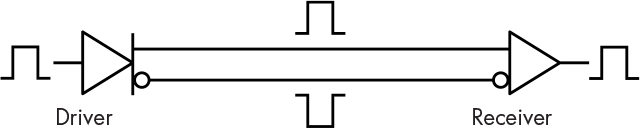
Figure 2-32: Differential signaling

You can see that there’s a driver that converts the input signal into complementary outputs, and a receiver that converts complementary inputs back into a single-ended output. It’s common for the receiver to include a Schmitt trigger for additional noise immunity.

Of course, there are limitations. Too much noise can push electronic components out of their specified operating range—imagine there’s a building next to the sidewalk and you and your friend both get pushed into the wall. A common-mode rejection ratio (CMRR) is part of a component specification and indicates the amount of noise that can be handled. It’s called “common-mode” because it refers specifically to noise that is common to both signals in a pair.

Differential signaling is used in many places, such as telephone lines. This application became necessary in the 1880s when electric streetcars made their debut, because they generated a lot of electrical noise that interfered with telephone signals. Scottish inventor Alexander Graham Bell (1847–1922) invented twisted-pair cabling, in which pairs of wires were twisted together for the electrical equivalent of snuggling (see Figure 2-33). He also patented the telephone. Today, twisted pair is ubiquitous; you’ll find it in USB, SATA (disk drive), and Ethernet cables.

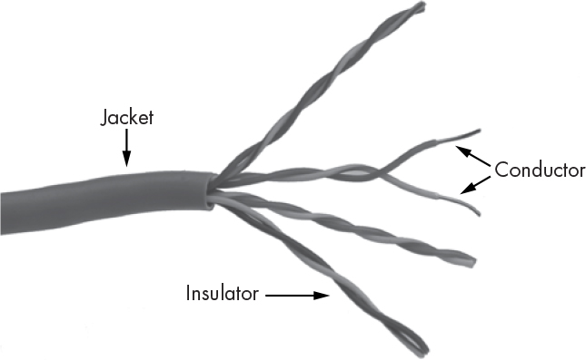
Figure 2-33: Twisted-pair Ethernet cable

An interesting application of differential signaling can be found in the Wall of Sound concert audio system used by the American band The Grateful Dead (1965–1995). It addressed the problem of vocal microphone feedback by using microphones in pairs wired so that the output from one microphone was subtracted from the output of the other. That way, any sound hitting both mics was common-mode and canceled out. Vocalists would sing into one of the mics in the pair so their voice would come through. An artifact of this system, which can be heard in the band’s live recordings, is that audience noise sounds tinny. That’s because lower-frequency sounds have longer wavelengths than higher-frequency sounds; lower-frequency noise is more likely to be common-mode than higher-frequency noise.

Propagation Delay

I touched on propagation delay back in “Using Plumbing to Understand Electricity” on page 41. Propagation delay is the amount of time it takes for a change in input to be reflected in the output. It is a statistical measure due to variances in manufacturing processes and temperature, plus the number and type of components connected to the output of a gate. Gates have both a minimum and maximum delay; the actual delay is somewhere in between. Propagation delay is one of the factors that limits the maximum speed that can be achieved in logic circuits. Designers have to use the worst-case values if they want their circuits to work. That means they have to design assuming the shortest and longest possible delays.

In Figure 2-34, gray areas indicate where we can’t rely on the outputs because of propagation delay.

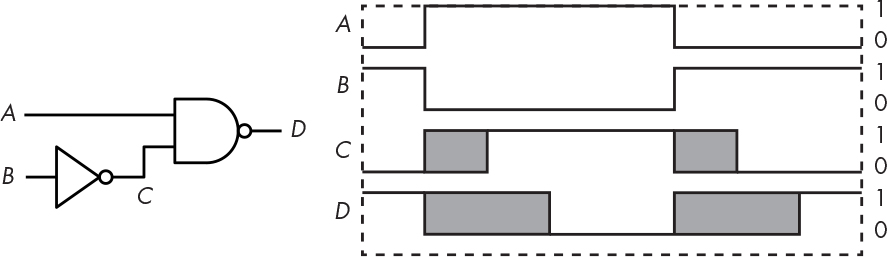
Figure 2-34: Propagation delay example

The outputs could change as early as the left edge of the gray regions, but they’re not guaranteed to change until the right edge. And the length of the gray areas increases as more gates are strung together.

There is a huge range of propagation delay times that depends on process technology. Individual components, such as 7400 series parts, can have delays in the 10-nanosecond range (that is, 10 billionths of a second). The gate delays inside modern large components, such as microprocessors, can be in picoseconds (trillionths of a second). If you’re reading the specifications for a component, the propagation delays are usually specified as t_PLH and t_PHL for the propagation time from low to high and high to low, respectively.

Now that we’ve discussed the inputs and what happens on the way to the outputs, it’s time to look at the outputs.

Output Variations

We’ve talked some about gate inputs, but we haven’t said much about outputs. There are a few different types of outputs designed for different applications.

Totem-Pole Output

A normal gate output is called a totem pole because the way in which one transistor is stacked on top of another resembles a totem pole. We can model this type of output using switches, as shown in Figure 2-35.

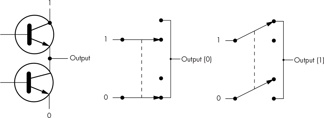
Figure 2-35: Totem-pole output

The schematic on the left illustrates how totem-pole outputs get their name. The top switch in the figure is called an active pull-up because it connects the output to the high logic level to get a 1 on the output. Totem-pole outputs can’t be connected together. As you can see in Figure 2-35, if you connected one with a 0 output to one with a 1 output, you would have connected the positive and negative power supplies together—which would be as bad as crossing the streams from the 1984 movie Ghostbusters and could melt the components.

Open-Collector Output

Another type of output is called open-collector or open-drain, depending on the type of transistor used. The schematic and switch model for this output are shown in Figure 2-36.

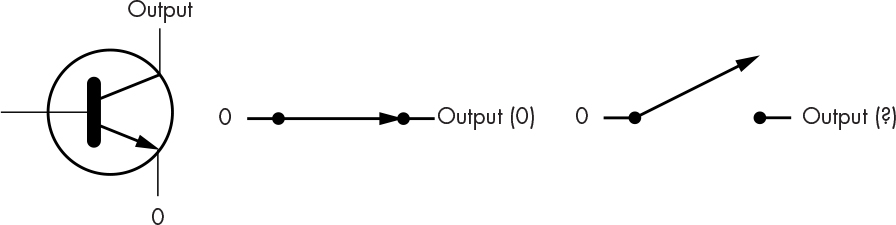
Figure 2-36: Open-collector/open-drain output

This seems odd at first glance. It’s fine if we want a 0 output, but when it’s not, 0 the output just floats, so we don’t know what its value is.

Because the open-collector and open-drain versions don’t have active pull-ups, we can connect their outputs together without harm. We can use a passive pull-up, which is just a pull-up resistor connecting the output to the supply voltage, which is the source of 1s. This is called V_CC for bipolar transistors and V_DD for MOS (metal-oxide-semiconductor) transistors. A passive pull-up has the effect of creating a wired-AND, shown in Figure 2-37.

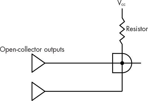
Figure 2-37: Wired-AND

What’s happening here is that when neither open-collector output is low, the resistor pulls the signal up to a 1. The resistor limits the current so that things don’t catch fire. The output is 0 when any of the open-collector outputs is low. You can wire a large number of things together this way, eliminating the need for an AND gate with lots of inputs.

Another use of open-collector and open-drain outputs is to drive devices like LEDs (light-emitting diodes). Open-collector and open-drain devices are often designed to support this use and can handle higher current than totem-pole devices. Some versions allow the output to be pulled up to a voltage level that is higher than the logic 1 level, which allows us to interface to other types of circuitry. This is important because although the threshold is consistent within a family of gates such as the 7400 series, other families have different thresholds.

Tri-State Output

Although open-collector circuits allow outputs to be connected together, they’re just not as fast as active pull-ups. So let’s move away from the two-state solution and introduce tri-state outputs. The third state is off. There is an extra enable input that turns the output on and off, as shown in Figure 2-38.

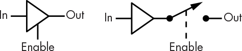
Figure 2-38: Tri-state output

Off is known as the hi-Z, or high-impedance, state. Z is the symbol for impedance, the mathematically complex version of resistance. You can imagine a tri-state output as the circuit from Figure 2-35. Controlling the bases separately gives us four combinations: 0, 1, hi-Z, and meltdown. Obviously, circuit designers must make sure that the meltdown combination cannot be selected.

Tri-state outputs allow a large number of devices to be hooked together. The caveat is that only one device can be enabled at a time.

Building More Complicated Circuits

The introduction of gates greatly simplified the hardware design process. People no longer had to design everything from discrete components. For example, where it took around 10 components to build a two-input NAND gate, the 7400 included four of them in a single package, called a small-scale integration (SSI) part, so that one package could replace 40.

Hardware designers could build anything from SSI gates just as they could using discrete components, which made things cheaper and more compact. And because certain combinations of gates are used a lot, medium-scale integration (MSI) parts were introduced that contained these combinations, further reducing the number of parts needed. Later came large-scale integration (LSI), very large-scale integration (VLSI), and so on.

You’ll learn about some of the gate combinations in the following sections, but this isn’t the end of the line. We use these higher-level functional building blocks themselves to make even higher-level components, similar to the way in which complex computer programs are constructed from smaller programs.

Building an Adder

Let’s build a two’s-complement adder. You may never need to design one of these, but this example will demonstrate how clever manipulation of logic can improve performance—which is true for both hardware and software.

We saw back in Chapter 1 that the sum of 2 bits is the XOR of those bits and the carry is the AND of those bits. Figure 2-39 shows the gate implementation.

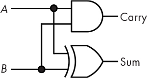
Figure 2-39: Half adder

You can see that the XOR gate provides the sum and the AND gate provides the carry. Figure 2-39 is called a half adder because something is missing. It’s fine for adding two bits, but there needs to be a third input so that we can carry. This means that two adders are needed to get the sum for each bit. We carry when at least two of the inputs are 1. Table 2-1 shows the truth table for this full adder.

Table 2-1: Truth Table for Full Adder

A	B	C	Sum	Carry
0	0	0	0	0
0	0	1	1	0
0	1	0	1	0
0	1	1	0	1
1	0	0	1	0
1	0	1	0	1
1	1	0	0	1
1	1	1	1	1

A full adder is a bit more complicated to build and looks like Figure 2-40.

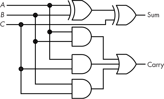
Figure 2-40: Full adder

As you can see, this takes many more gates. But now that we have the full adder, we can use it to build an adder for more than one bit. Figure 2-41 shows a configuration called a ripple-carry adder.

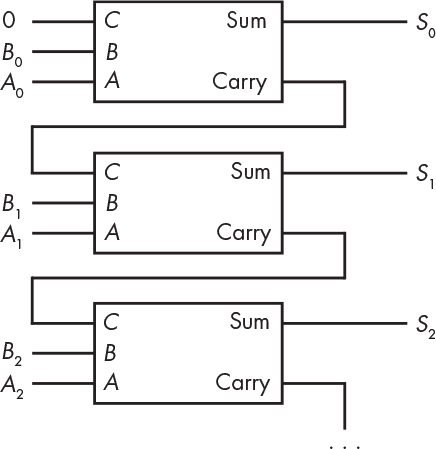
Figure 2-41: Ripple-carry adder

This ripple-carry adder gets its name from the way that the carry ripples from one bit to the next. It’s like doing the wave. This works fine, but you can see that there are two gate delays per bit, which adds up fast if we’re building a 32- or 64-bit adder. We can eliminate these delays with a carry look-ahead adder, which we can figure out how to make work using some basic arithmetic.

We can see in Figure 2-40 that the full-adder carry-out for bit i that is fed into the carry-in for bit i + 1:

C_i+1 = (A_i AND B_i) OR (A_i AND C_i) OR (B_i AND C_i)

The big sticking point here is that we need C_i in order to get C_i+1, which causes the ripple. You can see this in the following equation for C_i+2:

C_i+2 = (A_i+1 AND B_i+1) OR (A_i+1 AND C_i+1) OR (B_i+1 AND C_i+1)

We can eliminate this dependency by substituting the first equation into the second, as follows:

C_i+2 = (A_i+1 AND B_i+1)

OR(A_i+1 AND ((A_i AND B_i) OR (A_i AND C_i) OR (B_i AND C_i)))
OR(B_i+1 AND ((A_i AND B_i) OR (A_i AND C_i) OR (B_i AND C_i)))

Note that although there are a lot more ANDs and ORs, there’s still only two gates’ worth of propagation delay. C_n is dependent only on the A and B inputs, so the carry time, and hence the addition time, doesn’t depend on the number of bits. C_n can always be generated from C_n–1, which uses an increasingly large number of gates as n increases. Although gates are cheap, they do consume power, so there is a trade-off between speed and power consumption.

Building Decoders

In “Representing Integers Using Bits” on page 6, we built or encoded numbers from bits. A decoder does the opposite by turning an encoded number back into a set of individual bits. One application of decoders is to drive displays. You may have seen nixie tubes (shown in Figure 2-42) in old science fiction movies; they’re a really cool retro display for numbers. They’re essentially a set of neon signs, one for each digit. Each glowing wire has its own connection, requiring us to turn a 4-bit number into 10 separate outputs.

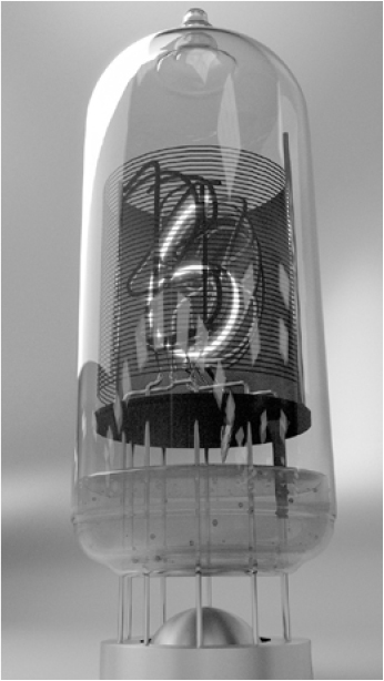
Figure 2-42: A nixie tube

Recall that octal representation takes eight distinct values and encodes them into 3 bits. Figure 2-43 shows a 3:8 decoder that converts an octal value back into a set of single bits.

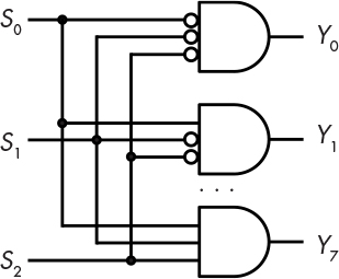
Figure 2-43: A 3:8 decoder

When the input is 000, the Y₀ input is true; when the input is 001, Y₁ is true; and so on. Decoders are principally named by the number of inputs and outputs. The example in Figure 2-43 has three inputs and eight outputs, so it’s a 3:8 decoder. This decoder would commonly be drawn as shown in Figure 2-44.

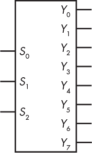
Figure 2-44: The 3:8 decoder schematic symbol

Building Demultiplexers

You can use a decoder to build a demultiplexer, commonly abbreviated as dmux, which allows an input to be directed to one of several outputs, as you would do if sorting Hogwarts students into houses. A demultiplexer combines a decoder with some additional gates, as shown in Figure 2-45.

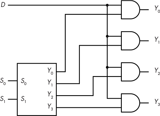
Figure 2-45: A 1:4 demultiplexer

The demultiplexer directs the input signal D to one of the four outputs Y_0–3 based on the decoder inputs S_0–1. The symbol in Figure 2-46 is used in schematics for demultiplexers.

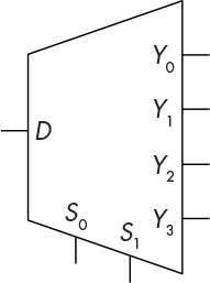
Figure 2-46: The demultiplexer schematic symbol

Building Selectors

Choosing one input from a number of inputs is another commonly performed function. For example, we might have several operand sources for an adder and need to choose one. Using gates, we can create another functional block called a selector or multiplexer (mux).

A selector combines a decoder with some additional gates, as shown in Figure 2-47.

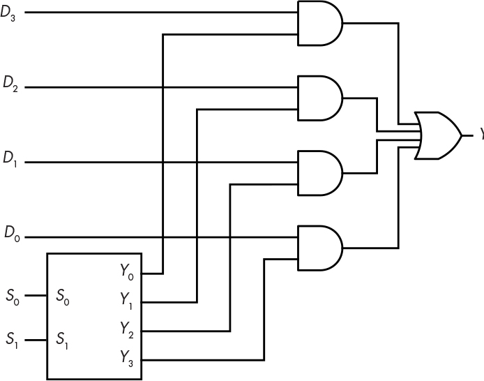
Figure 2-47: A 4:1 selector

Selectors are also used a lot and have their own schematic symbol. Figure 2-48 shows the symbol for a 4:1 selector, which is pretty much the reverse of the symbol for a decoder.

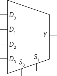
Figure 2-48: The 4:1 selector schematic symbol

You’re probably familiar with selectors but don’t know it. You might have a toaster oven that has a dial with positions labeled Off, Toast, Bake, and Broil. That’s a selector switch with four positions. A toaster oven has two heating elements, one on top and another on the bottom. Toaster oven logic works as shown in Table 2-2.

Table 2-2: Toaster Oven Logic

Setting	Top element	Bottom element
Off	Off	Off
Bake	Off	On
Toast	On	On
Broil	On	Off

We can implement this logic using a pair of 4:1 selectors ganged together, as shown in Figure 2-49.

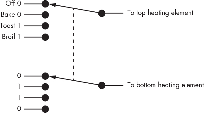
Figure 2-49: Toaster oven selector switch

Summary

In this chapter, you learned why we use bits instead of digits to build hardware. You also saw some of the developments in technology that have allowed us to implement bits and combinatorial digital logic. You learned about modern logic design symbols and how simple logic elements can be combined to make more complex devices. We looked at how the outputs of combinatorial devices are a function of their inputs, but because the outputs change in response to the inputs, there’s no way to remember anything. Remembering requires the ability to “freeze” an output so that it doesn’t change in response to inputs. Chapter 3 discusses sequential logic, which enables us to remember things over time.