8
LANGUAGE PROCESSING

It’s pretty clear that only crazy people would try to write computer programs. That’s always been true, but programming languages at least make the job a lot easier.
This chapter examines how programming languages are implemented. Its aim is to help you develop an understanding of what happens with your code. You’ll also learn how the code you write is transformed into an executable form called machine language.
Assembly Language
We saw a machine language implementation of a program to compute Fibonacci numbers back in Table 4-4 on page 108. As you might imagine, figuring out all the bit combinations for instructions is pretty painful. Primitive computer programmers got tired of this and came up with a better way to write computer programs, called assembly language.
Assembly language did a few amazing things. It let programmers use mnemonics for instructions so they didn’t have to memorize all the bit combinations. It allowed them to give names or labels to addresses. And it allowed them to include comments that can help other people read and understand the program.
A program called an assembler reads assembly language programs and produces machine code from them, filling in the values of the labels or symbols as it goes. This is especially helpful because it prevents dumb errors caused by moving things around.
Listing 8-1 shows what the Fibonacci program from Table 4-4 looks like in the hypothetical assembly language from Chapter 4.
load #0 ; zero the first number in the sequence
store first
load #1 ; set the second number in the sequence to 1
store second
again: load first ; add the first and second numbers to get the
add second ; next number in the sequence
store next
; do something interesting with the number
load second ; move the second number to be the first number
store first
load next ; make the next number the second number
store second
cmp #200 ; are we done yet?
ble again ; nope, go around again
first: bss 1 ; where the first number is stored
second: bss 1 ; where the second number is stored
next: bss 1 ; where the next number is stored
Listing 8-1: Assembly language program to compute the Fibonacci sequence
The bss (which stands for block started by symbol) pseudo-instruction reserves a chunk of memory—in this case, one address—without putting anything in that location. Pseudo-instructions don’t have a direct correspondence with machine language instructions; they’re instructions to the assembler. As you can see, assembly language is much easier to deal with than machine language, but it’s still pretty tedious stuff.
Early programmers had to pull themselves up by their own bootstraps. There was no assembler to use when the first computer was made, so programmers had to write the first one the hard way, by figuring out all the bits by hand. This first assembler was quite primitive, but once it worked, it could be used to make a better one, and so on.
The term bootstrap has stuck around, although it’s often shortened to boot. Booting a computer often involves loading a small program, which loads a bigger one, which in turn loads an even bigger one. On early computers, people had to enter the initial bootstrap program by hand, using switches and lights on the front panel.
High-Level Languages
Assembly language helped a lot, but as you can see, doing simple things with it still takes a lot of work. We’d really like to be able to use fewer words to describe more complicated tasks. Fred Brooks’s 1975 book The Mythical Man-Month: Essays on Software Engineering (Addison-Wesley) claims that on average, a programmer can write 3 to 10 lines of documented, debugged code per day. So a lot more work could get done if a line of code did more.
Enter high-level languages, which operate at a higher level of abstraction than assembly language. Source code in high-level languages is run through a program called a compiler, which translates or compiles it into machine language, also known as object code.
Thousands of high-level languages have been invented. Some are very general, and some are designed for specific tasks. One of the first high-level languages was called FORTRAN, which stood for “formula translator.” You could use it to easily write programs that solved formulas like y = m × x + b. Listing 8-2 shows what our Fibonacci sequence program would look like in FORTRAN.
C SET THE INITIAL TWO SEQUENCE NUMBERS IN I and J
I=0
J=1
C GET NEXT SEQUENCE NUMBER
5 K=I+J
C DO SOMETHING INTERESTING WITH THE NUMBER
C SHIFT THE SEQUENCE NUMBERS TO I AND J
I=J
J=K
C DO IT AGAIN IF THE LAST NUMBER WAS LESS THAN 200
IF (J .LT. 200) GOTO 5
C ALL DONE
Listing 8-2: Fibonacci sequence program in FORTRAN
Quite a bit simpler than assembly language, isn’t it? Note that lines that begin with the letter C are comments. And although we have labels, they must be numbers. Also note that we don’t have to explicitly declare memory that we want to use—it just magically appears when we use variables such as I and J. FORTRAN did something interesting (or ugly, depending on your point of view) that still reverberates today. Any variable name that began with the letter I, J, K, L, M, or N was an integer, which was borrowed from the way mathematicians write proofs. Variables beginning with any other letter were floating-point, or REAL in FORTRAN-speak. Generations of former FORTRAN programmers still use i, j, k, l, m, and n or their upper-case equivalents as names for integer variables.
FORTRAN was a pretty cumbersome language that ran on the really big machines of the time. As smaller, cheaper machines became available (that is, ones that only took up a small room), people came up with other languages. Most of these new languages, such as BASIC (which stood for “Beginner’s All-purpose Symbolic Instruction Code”), were variations on the FORTRAN theme. All of these languages suffered from the same problem. As programs increased in complexity, the network of line numbers and GOTOs became an unmanageable tangle. People would write programs with the label numbers all in order and then have to make a change that would mess it up. Many programmers started off by using labels 10 or 100 apart so that they’d have room to backfill later, but even that didn’t always work.
Structured Programming
Languages like FORTRAN and BASIC are called unstructured because there is no structure to the way that labels and GOTOs are arranged. You can’t build a house by throwing a pile of lumber on the ground in real life, but you can in FORTRAN. I’m talking about original FORTRAN; over time, the language has evolved and incorporated structured programming. It’s still the most popular scientific language.
Structured programming languages were developed to address this spaghetti code problem by eliminating the need for the nasty GOTO. Some went too far. For example, Pascal got rid of it completely, resulting in a programming language that was useful only for teaching elementary structured programming. To be fair, that’s actually what it was designed to do. C, the successor to the Ken Thompson’s B, was originally developed by Dennis Ritchie at Bell Telephone Laboratories. It was very pragmatic and became one of the most widely used programming languages. A large number of later languages—including C++, Java, PHP, Python, and JavaScript—copied elements from C.
Listing 8-3 shows how our Fibonacci program might appear in JavaScript. Note the absence of explicit branching.
var first; // first number
var second; // second number
var next; // next number in sequence
first = 0;
second = 1;
while ((next = first + second) < 200) {
// do something interesting with the number
first = second;
second = next;
}
Listing 8-3: JavaScript program to compute Fibonacci sequence
The statements inside the curly brackets {} are executed as long as the while condition in the parentheses is true. Execution continues after the } when that condition becomes false. The flow of control is cleaner, making the program easier to understand.
Lexical Analysis
Now let’s look at what it takes to process a language. We’ll start with lexical analysis, the process of converting symbols (characters) into tokens (words).
A simple way of looking at lexical analysis is to say that a language has two types of tokens: words and separators. For example, using the above rules, lex luthor (the author of all evil programming languages) has two word tokens (lex and luthor) and one separator token (the space). Figure 8-1 shows a simple algorithm that divides its input into tokens.
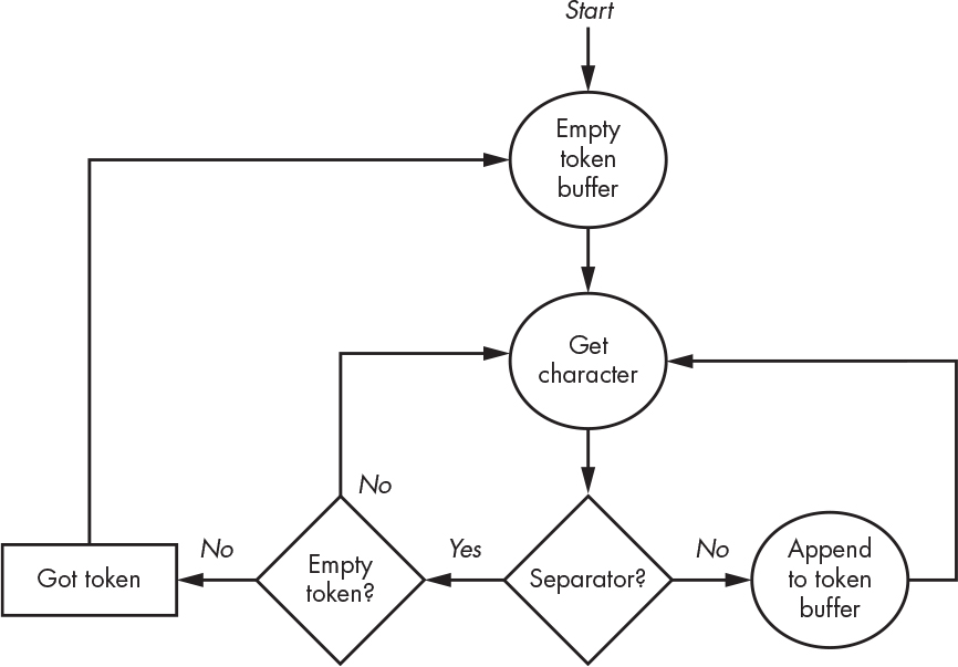
Figure 8-1: Simple lexical analysis
It’s not enough to just extract tokens; we need to classify them because practical languages have many different types of tokens, such as names, numbers, and operators. Languages typically have operators and operands, just like math, and operands can be variables or constants (numbers). The free-form nature of many languages also complicates things—for example, when separators are implied, as in A+B as opposed to A + B (note the spaces). Both forms have the same interpretation, but the first form doesn’t have any explicit separators.
Numeric constants are astonishingly hard to classify, even if we ignore the distinctions among octal, hexadecimal, integer, and floating-point numbers. Let’s diagram what constitutes a legitimate floating-point number. There are many ways to specify a floating-point number, including 1., .1, 1.2, +1.2, –.1, 1e5, 1e+5, 1e–5, and 1.2E5, as shown in Figure 8-2.
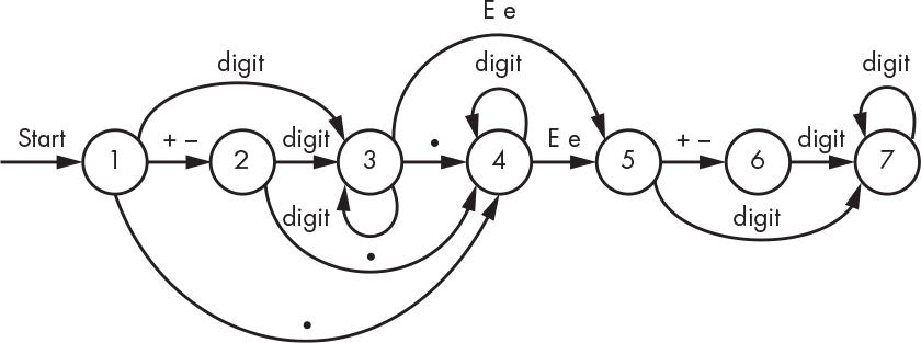
Figure 8-2: Diagram for floating-point numbers
We start at the bubble labeled 1. A + or – character brings us to bubble 2, while a . sends us to bubble 4. We leave bubble 2 for bubble 4 when we get a . character, but we go to bubble 3 when we receive a digit. Bubbles 3 and 4 accumulate digits. We’re done if we get a character for which no transition is shown. For example, if we received a space while at any of the bubbles, we’d be done. Of course, leaving bubble 2 without a digit or decimal point, bubble 6 without a digit, or bubble 5 without a sign or digit is an error because it doesn’t produce a complete floating-point number. These paths are absent from the diagram for simplicity’s sake.
This is a lot like trying to find treasure using a pirate map. As long as you’re following directions, you can get from one place to another. If you don’t follow directions—for example, with a Z at bubble 1—you fall off the map and get lost.
You could view Figure 8-2 as the specification for floating-point numbers and write software to implement it. There are other, more formal ways to write specifications, however, such as Backus-Naur form.
State Machines
Based just on the complexity of numbers, you can imagine that it would take a substantial amount of special case code to extract language tokens from input. Figure 8-2 gave us a hint that there’s another approach. We can construct a state machine, which consists of a set of states and a list of what causes a transition from one state to another—exactly what we saw in Figure 8-2. We can arrange this information as shown in Table 8-1.
Table 8-1: State Table for Floating-Point Numbers
Input |
State |
||||||
1 |
2 |
3 |
4 |
5 |
6 |
7 |
|
0 |
3 |
3 |
3 |
4 |
7 |
7 |
7 |
1 |
3 |
3 |
3 |
4 |
7 |
7 |
7 |
2 |
3 |
3 |
3 |
4 |
7 |
7 |
7 |
3 |
3 |
3 |
3 |
4 |
7 |
7 |
7 |
4 |
3 |
3 |
3 |
4 |
7 |
7 |
7 |
5 |
3 |
3 |
3 |
4 |
7 |
7 |
7 |
6 |
3 |
3 |
3 |
4 |
7 |
7 |
7 |
7 |
3 |
3 |
3 |
4 |
7 |
7 |
7 |
8 |
3 |
3 |
3 |
4 |
7 |
7 |
7 |
9 |
3 |
3 |
3 |
4 |
7 |
7 |
7 |
e |
error |
error |
5 |
5 |
error |
error |
done |
E |
error |
error |
5 |
5 |
error |
error |
done |
+ |
2 |
error |
done |
done |
6 |
error |
done |
– |
2 |
error |
done |
done |
6 |
error |
done |
. |
4 |
4 |
4 |
done |
error |
error |
done |
other |
error |
error |
done |
done |
error |
error |
done |
Looking at the table, you can see that when we’re in state 1, digits move us to state 3, e or E moves us to state 5, + or – to state 2, and . to state 4—anything else is an error.
Using a state machine allows us to classify the input using a simple piece of code, as shown in Listing 8-4. Let’s use Table 8-1, replacing done with 0 and error with -1. For simplicity, we’ll have an other row in the table for each of the other characters.
state = 1;
while (state > 0)
state = state_table[state][next_character];
Listing 8-4: Using a state machine
This approach could easily be expanded to other types of tokens. Rather than have a single value for done, we could have a different value for each type of token.
Regular Expressions
Building tables like Table 8-1 from diagrams like Figure 8-2 is very cumbersome and error-prone for complicated languages. The solution is to create languages for specifying languages. American mathematician Stephen Cole Kleene (1909–1994) supplied the mathematical foundation for this approach way back in 1956. Ken Thompson first converted it into software in 1968 as part of a text editor and then created the UNIX grep (which stands for “globally search a regular expression and print”) utility in 1974. This popularized the term regular expression, which is now ubiquitous. Regular expressions are languages themselves, and of course there are now several incompatible regular expression languages. Regular expressions are a mainstay of pattern matching. Figure 8-3 shows a regular expression that matches the pattern for a floating-point number.
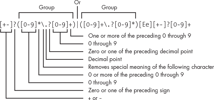
Figure 8-3: Regular expression for floating-point number
This looks like gibberish but really only relies on a few simple rules. It’s processed from left to right, meaning that the expression abc would match the string of characters “abc”. If something in the pattern is followed by ?, it means zero or one of those things, * means zero or more, and + means one or more. A set of characters enclosed in square brackets matches any single character in that set, so [abc] matches a, b, or c. The . matches any single character and so needs to be escaped with a backslash () so that it matches the . character only. The | means either the thing on the left or the thing on the right. Parentheses () are for grouping, just like in math.
Reading from left to right, we start with an optional plus or minus sign. This is followed by either zero or more digits, an optional decimal point, and one or more digits (which handles cases like 1.2 and .2), or by one or more digits, an optional decimal point, and zero or more digits (which handles the 1 and 1. cases). This is followed by the exponent, which begins with an E or e, followed by an optional sign and one or more digits. Not as horrible as it first looked, is it?
Having a regular expression language that processed input into tokens would be more useful if it automatically generated state tables. And we have one, thanks again to research at Bell Telephone Laboratories. In 1975, American physicist Mike Lesk—along with intern Eric Schmidt, who today is executive chairman of Google’s parent company, Alphabet—wrote a program called lex, short for “lexical analyzer.” As The Beatles said in “Penny Lane:” “It’s a Kleene machine.” An open source version called flex was later produced by the GNU project. These tools do exactly what we want. They produce a state table driven program that executes user-supplied program fragments when input matches regular expressions. For example, the simple lex program fragment in Listing 8-5 prints ah whenever it encounters either ar or er in the input and prints er whenever it encounters an a at the end of a word.
[ae]r printf("ah");
a/[ .,;!?] printf("er");
Listing 8-5: Bostonian lex program fragment
The / in the second pattern means “only match the thing on its left if it is followed by the thing on its right.” Things not matched are just printed. You can use this program to convert regular American English to Bostonian: for example, inputting the text Park the car in Harvard yard and sit on the sofa would produce Pahk the cah in Hahvahd yahd and sit on the sofer as output.
Classifying tokens is a piece of cake in lex. For example, Listing 8-6 shows some lex that matches all of our number forms plus variable names and some operators. Instead of printing out what we find, we return some values defined elsewhere for each type of token. Note that several of the characters have special meaning to lex and therefore require the backslash escape character so that they’re treated as literals.
0[0-7]* return (INTEGER);
[+-]?[0-9]+ return (INTEGER);
[+-]?(([0-9]*.?[0-9]+)|([0-9]+.?[0-9]*))([Ee][+-]?[0-9]+)? return (FLOAT);
0x[0-9a-fA-F]+ return (INTEGER);
[A-Za-z][A-Za-z0-9]* return (VARIABLE);
+ return (PLUS);
- return (MINUS);
* return (TIMES);
/ return (DIVIDE);
= return (EQUALS);
Listing 8-6: Classifying tokens using lex
Not shown in the listing is the mechanism by which lex supplies the actual values of the tokens. When we find a number, we need to know its value; likewise, when we find a variable name, we need to know that name.
Note that lex doesn’t work for all languages. As computer scientist Stephen C. Johnson (introduced shortly) explained, “Lex can be easily used to produce quite complicated lexical analyzers, but there remain some languages (such as FORTRAN) which do not fit any theoretical framework, and whose lexical analyzers must be crafted by hand.”
From Words to Sentences
So far, we’ve seen how we can turn sequences of characters into words. But that’s not enough for a language. We now need to turn those words into sentences according to some grammar.
Let’s use the tokens from Listing 8-6 to create a simple four-function calculator. Expressions such as 1 + 2 and a = 5 are legal, whereas 1 + + + 2 isn’t. We once again find ourselves in need of pattern matching, but this time for token types. Maybe somebody has already thought about this.
That somebody would be Stephen C. Johnson, who also—unsurprisingly—worked at Bell Labs. He created yacc (for “yet another compiler compiler”) in the early 1970s. The name should give you an idea of how many people were playing with these sorts of things back then. It’s still in use today; an open source version, called bison, is available from the GNU project. Just like lex, yacc and bison generate state tables and the code to operate on them.
The program yacc generates is a shift-reduce parser using a stack (see “Stacks” on page 122). In this context, shift means pushing a token onto the stack, and reduce means replacing a matched set of tokens on the stack with a token for that set. Look at the BNF for the calculator in Listing 8-7—it uses the token values produced by lex in Listing 8-6.
<operator> ::= PLUS | MINUS | TIMES | DIVIDE
<operand> ::= INTEGER | FLOAT | VARIABLE
<expression> ::= <operand> | <expression> PLUS <operand>
| <expression> MINUS <operand>
| <expression> TIMES <operand>
| <expression> DIVIDE <operand>
<assignment> ::= <variable> EQUALS <expression>
<statement> ::= <expression> | <assignment>
<statements> ::= "" | <statements> <statement>
<calculator> ::= <statements>
Listing 8-7: Simple calculator BNF
Shift-reduce is easy to understand once you see it in action. Look at what happens when our simple calculator is presented with the input 4 + 5 – 3 in Figure 8-4. Referring back to “Different Equation Notations” on page 125, you can see that processing infix notion equations requires a deeper stack than postfix (RPN) requires because more tokens, such as parentheses, must be shifted before anything can be reduced.
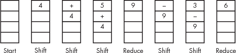
Figure 8-4: Shift-reduce in action
Listing 8-8 shows what our calculator would look like when coded in yacc. Note the similarity to the BNF. This is for illustration only; it’s not a fully working example, as that would introduce far too many nitpicky distractions.
calculator : statements
;
statements : /* empty */
| statement statements
;
operand : INTEGER
| FLOAT
| VARIABLE
;
expression : expression PLUS operand
| expression MINUS operand
| expression TIMES operand
| expression DIVIDE operand
| operand
;
assignment : VARIABLE EQUALS expression
;
statement : expression
| assignment
;
Listing 8-8: Partial yacc for a simple calculator
The Language-of-the-Day Club
Languages used to be difficult. In 1977, Canadian computer scientist Alfred Aho and American computer scientist Jeffrey Ullman at Bell Labs published Principles of Compiler Design, one of the first computer-typeset books published using the troff typesetting language. One can summarize the book as follows: “languages are hard, and you had better dive into the heavy math, set theory, and so on.” The second edition, published in 1986 along with Indian computer scientist Ravi Sethi, had a completely different feel. Its attitude was more like “languages are a done thing, and here’s how to do them.” And people did.
That edition popularized lex and yacc. All of a sudden, there were languages for everything—and not just programming languages. One of my favorite small languages was chem, by Canadian computer scientist Brian Kernighan at Bell Labs, which drew pretty chemical structure diagrams from input like C double bond O. The diagrams in the book you’re reading, in fact, were created using Brian Kernighan’s picture-drawing language pic.
Creating new languages is fun. Of course, people started making new languages without understanding their history and reintroduced old mistakes. For example, many consider the handling of whitespace (the spaces between words) in the Ruby language to be a replay of a mistake in the original C language that was fixed long ago. (Note that one of the classic ways to deal with a mistake is to call it a feature.)
The result of all this history is that a huge number of languages are now available. Most don’t really add much value and are just demonstrations of the designer’s taste. It’s worth paying attention to domain-specific languages, particularly little languages such as pic and chem, to see how specific applications are addressed. American computer scientist Jon Bentley published a wonderful column about little languages called “Programming Pearls” in Communications of the ACM back in 1986. These columns were collected and published in updated book form in 1999 as Programming Pearls (Addison-Wesley).
Parse Trees
Earlier I talked about compiling high-level languages, but that’s not the only option. High-level languages can be compiled or interpreted. The choice is not a function of the design of the language but rather of its implementation.
Compiled languages produce machine code like you saw back in Table 4-4 page 108. The compiler takes the source code and converts it into machine language for a particular machine. Many compilers allow you to compile the same program for different target machines. Once a program is compiled, it’s ready to run.
Interpreted languages don’t result in machine language for a real machine (“real” as in hardware). Instead, interpreted languages run on virtual machines, which are machines written in software. They may have their own machine language, but it’s not a computer instruction set implemented in hardware. Note that the term virtual machine has become overloaded recently; I’m using it to mean an abstract computing machine. Some interpreted languages are executed directly by the interpreter. Others are compiled into an intermediate language for later interpretation.
In general, compiled code is faster because once it’s compiled, it’s in machine language. It’s like translating a book. Once it’s done, anyone who speaks that language can read it. Interpreted code is ephemeral, like someone reading a book aloud while translating it into the listener’s language. If another person later wants the book read to them in their own language, it must be translated again. However, interpreted code allows languages to have features that are really difficult to build in hardware. Computers are fast enough that we can often afford the speed penalty that comes with interpreters.
Figure 8-4 depicted the calculator directly executing the input. Although this is fine for something like a calculator, it skips a major step used for compilers and interpreters. For those cases, we construct a parse tree, which is a DAG (directed acyclic graph) data structure from the calculator grammar. We’ll build this tree out of node structures, as depicted in Figure 8-5.

Figure 8-5: Parse tree node layout
Each node includes a code that indicates the type of node. There is also an array of leaves; the interpretation of each leaf is determined by the code. Each leaf is a union since it can hold more than one type of data. We’re using C language syntax for the member naming, so, for example, .i is used if we’re interpreting a leaf as an integer.
We’ll assume the existence of a makenode function that makes new nodes. It takes a leaf count as its first argument, a code as its second, and the values for each leaf afterward.
Let’s flesh out the code from Listing 8-8 a bit more while still omitting some of the picky details. To keep things simple, we’ll only handle integer numbers. What was missing earlier was code to execute when matching grammar rules. In yacc, the value of each of the right-hand-side elements is available as $1, $2, and so on, and $$ is what gets returned by the rule. Listing 8-9 shows a more complete version of our yacc calculator.
calculator : statements { do_something_with($1); }
;
statements : /* empty */
| statement statements { $$.n = makenode(2, LIST, $1, $2); }
;
operand : INTEGER { $$ = makenode(1, INTEGER, $1); }
| VARIABLE { $$ = makenode(1, VARIABLE, $1); }
;
expression : expression PLUS operand { $$.n = makenode(2, PLUS, $1, $3); }
| expression MINUS operand { $$.n = makenode(2, MINUS, $1, $3); }
| expression TIMES operand { $$.n = makenode(2, TIMES, $1, $3); }
| expression DIVIDE operand { $$.n = makenode(2, DIVIDE, $1, $3); }
| operand { $$ = $1; }
;
assignment : VARIABLE EQUALS expression { $$.n = makenode(2, EQUALS, $1, $3); }
;
statement : expression { $$ = $1; }
| assignment { $$ = $1; }
;
Listing 8-9: Simple calculator parse tree construction using yacc
Here, all the simple rules just return their values. The more complicated rules for statements, expression, and assignment create a node, attach the children, and return that node. Figure 8-6 shows what gets produced for some sample input.

Figure 8-6: Simple calculator parse tree
As you can see, the code generates a tree. At the top level, we use the calculator rule to create a linked list of statements out of tree nodes. The remainder of the tree consists of statement nodes that contain the operator and operands.
Interpreters
Listing 8-9 includes a mysterious do_something_with function invocation that is passed the root of the parse tree. That function causes an interpreter to “execute” the parse tree. The first part of this execution is the linked-list traversal, as shown in Figure 8-7.
The second part is the evaluation, which we do recursively using depth-first traversal. This function is diagrammed in Figure 8-8.

Figure 8-7: Parse tree linked-list traversal

Figure 8-8: Parse tree evaluation
As you can see, it’s easy to decide what to do since we have a code in our node. Observe that we need an additional function to store a variable (symbol) name and value in a symbol table and another to look up the value associated with a variable name. These are commonly implemented using hash tables (see “Making a Hash of Things” on page 213).
Gluing the list traversal and evaluation code into yacc allows us to immediately execute the parse tree. Another option is to save the parse tree in a file where it can be read and executed later. This is how languages such as Java and Python work. For all intents and purposes, this is a set of machine language instructions, but for a machine implemented in software instead of hardware. A program that executes the saved parse tree must exist for every target machine. Often the same interpreter source code can be compiled and used for multiple targets.
Figure 8-9 summarizes interpreters.
The front end generates the parse tree, which is represented by some intermediate language, and the back ends are for various machines to execute that language in their target environments.

Figure 8-9: Interpreter structure
Compilers
Compilers look a lot like interpreters, but they have code generators instead of backend execution code, as shown in Figure 8-10.
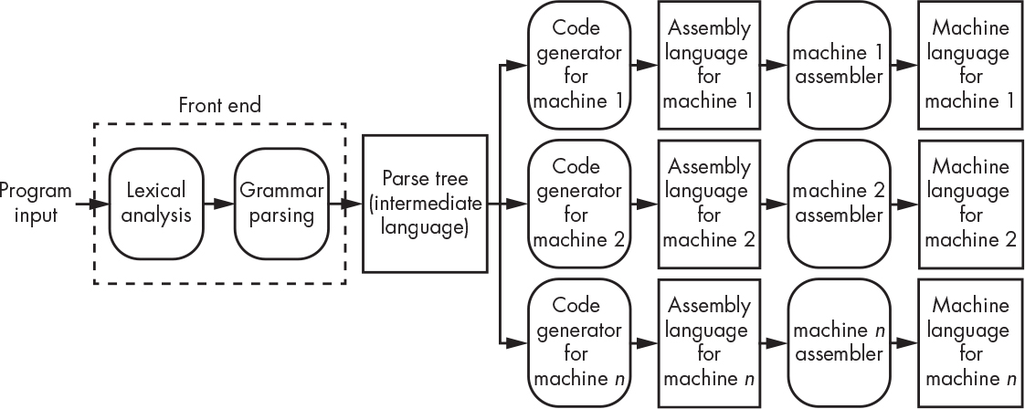
Figure 8-10: Compiler structure
A code generator generates machine language for a particular target machine. The tools for some languages, such as C, can generate the actual assembly language (see “Assembly Language” on page 217) for the target machine, and the assembly language is then run through that machine’s assembler to produce machine language.
A code generator looks exactly like the parse tree traversal and evaluation we saw in Figures 8-7 and 8-8. The difference is that the rectangles in Figure 8-8 are replaced by ones that generate assembly language instead of executing the parse tree. A simplified version of a code generator is shown in Figure 8-11; things shown in bold monospace font (like add tmp) are emitted machine language instructions for our toy machine from Chapter 4. Note that the machine there didn’t have multiply and divide instructions but, for this example, we pretend that it does.
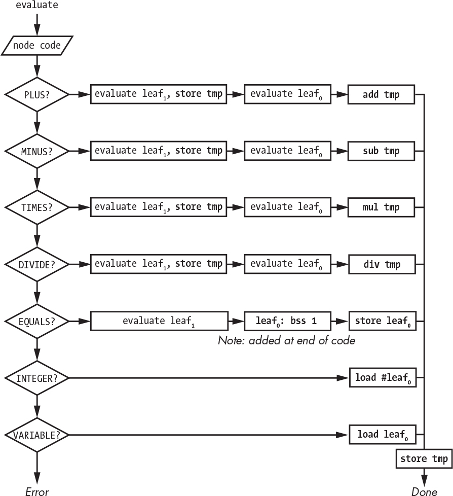
Figure 8-11: Assembler generation from parse tree
Applying Figure 8-11 to the parse tree in Figure 8-6, we get the assembly language program shown in Listing 8-10.
; first list element
load #3 ; grab the integer 3
store tmp ; save it away
load #2 ; grab the integer 2
mul tmp ; multiply the values subtree nodes
store tmp ; save it away
load #1 ; grab the integer 1
add tmp ; add it to the result of 2 times 3
store tmp ; save it away
; second list element
load #5 ; grab the integer 5
store foo ; save it in the space for the "foo" variable
store tmp ; save it away
; third list element
load foo ; get contents of "foo" variable
store tmp ; save it away
load #6 ; grab the integer 6
div tmp ; divide them
store tmp ; save it away
tmp: bss 1 ; storage space for temporary variable
foo: bss 1 ; storage space for "foo" variable
Listing 8-10: Machine language output from code generator
As you can see, this generates fairly bad-looking code; there are a lot of unnecessary loads and stores. But what can you expect from a contrived simple example? This code would be much improved via optimization, which is discussed in the next section.
This code can be executed once it’s assembled into machine language. It will run much faster than the interpreted version because it’s a much smaller and more efficient piece of code.
Optimization
Many language tools include an additional step called an optimizer between the parse tree and the code generator. The optimizer analyzes the parse tree and performs transformations that result in more efficient code. For example, an optimizer might notice that all the operands in the parse tree on the left in Figure 8-12 are constants. It can then evaluate the expression in advance at compile time so that evaluation doesn’t have to be done at runtime.
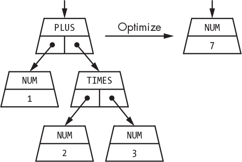
Figure 8-12: Optimizing a parse tree
The preceding example is trivial because our example calculator doesn’t include any way to do conditional branching. Optimizers have a whole bag of tricks. For example, consider the code shown in Listing 8-11 (which happens to be in C).
for (i = 0; i < 10; i++) {
x = a + b;
result[i] = 4 * i + x * x;
}
Listing 8-11: C loop code with assignment in loop
Listing 8-12 shows how an optimizer might restructure it.
x = a + b;
optimizer_created_temporary_variable = x * x;
for (i = 0; i < 10; i++) {
result[i] = 4 * i + optimizer_created_temporary_variable;
}
Listing 8-12: Loop code with loop invariant optimization
This example gives the same results as Listing 8-11 but is more efficient. The optimizer determined that a + b was loop invariant, meaning that its value didn’t change inside the loop. The optimizer moved it outside the loop so it would need to be computed only once instead of 10 times. It also determined that x * x was constant inside the loop and moved that outside.
Listing 8-13 shows another optimizer trick called strength reduction, which is the process of replacing expensive operations with cheaper ones—in this case, multiplication with addition.
x = a + b;
optimizer_created_temporary_variable = x * x;
optimizer_created_4_times_i = 0;
for (i = 0; i < 10; i++) {
result[i] = optimizer_created_4_times_i + optimizer_created_temporary_variable;
optimizer_created_4_times_i = optimizer_created_4_times_i + 4;
}
Listing 8-13: C loop code with loop-invariant optimization and strength reduction
Strength reduction could also take advantage of relative addressing to make the calculation of result[i] more efficient. Going back to Figure 7-2, result[i] is the address of result plus i times the size of the array element. Just like with the optimizer_created_4_times_i, we could start with the address of result and add the size of the array element on each loop iteration instead of using a slower multiplication.
Be Careful with Hardware
Optimizers are wonderful, but they can cause unexpected problems with code that manipulates hardware. Listing 8-14 shows a variable that’s actually a hardware register that turns on a light when bit 0 is set, like we saw back in Figure 6-1.
void
lights_on()
{
PORTB = 0x01;
return;
}
Listing 8-14: Example of code that shouldn’t be optimized
This looks great, but what’s the optimizer going to do? It will say, “Hey, this is being written but never read, so I can just get rid of it.” Likewise, say we have the code in Listing 8-15, which turns on the light and then tests to see whether or not it’s on. The optimizer would likely just rewrite the function to return 0x01 without ever storing it in PORTB.
unsigned int
lights_on()
{
PORTB = 0x01;
return (PORTB);
}
Listing 8-15: Another example of code that shouldn’t be optimized
These examples demonstrate that you need to be able to turn off optimization in certain cases. Traditionally, you’d do so by splitting up the software into general and hardware-specific files and running the optimizer only on the general ones. However, some languages now include mechanisms that allow you to tell the optimizer to leave certain things alone. For example, in C the volatile keyword says not to optimize access to a variable.
Summary
So far in this book, you’ve learned how computers work and how they run programs. In this chapter, you saw how programs get transformed so that they can be run on machines and learned that programs can be compiled or interpreted.
In the next chapter, you’ll meet a monster of an interpreter called a web browser and the languages that it interprets.