
CHAPTER 2
INFERENCE PROBLEMS
With the valuation algebra framework introduced in the first chapter, we dispose of a system to express the structure of information independently of any concrete formalism. This system will now be used to describe the main computational problem of knowledge representation systems: the task of computing inference. Let us go back to our initial idea of valuations as pieces of knowledge or information. Given a collection of information pieces called knowledgebase and some query of interest, inference consists in aggregating all elements of the knowledgebase, followed by projecting the result to a specified domain representing the question of interest. This computational problem called inference or projection problem will take center stage in many of the following chapters. Here, we start with a short presentation of some important graphical structures used to represent knowledgebases and to uncover their hidden structure. Then, we give a formal definition of inference problems in Section 2.3, followed by a selection of examples that arise from the valuation algebra instances of Chapter 1. Most interesting are the different meanings that the inference problem adopts under different valuation algebras. We therefore not only say that formalisms instantiate valuation algebras, but the computational problems based on these formalisms also instantiate the generic inference problem. Algorithms for the efficient solution of inference problems will be presented in Chapter 3 and 4.
2.1 GRAPHS, TREES AND HYPERGRAPHS
An undirected graph G = (V, E) is specified by a set of vertices or nodes V and a set of edges E. Edges are sets of either one or two nodes, i.e. E ![]() V1 ∪ V2 where V1 denotes the set of all one-element subsets and V2 the set of all two-element subsets of V. Without loss of generality, we subsequently identify nodes by natural numbers
V1 ∪ V2 where V1 denotes the set of all one-element subsets and V2 the set of all two-element subsets of V. Without loss of generality, we subsequently identify nodes by natural numbers ![]() . The neighbors of node
. The neighbors of node ![]() are all other nodes with an edge to node
are all other nodes with an edge to node ![]() , and the degree of a graph G is the maximum number of neighbors over all its nodes:
, and the degree of a graph G is the maximum number of neighbors over all its nodes:
(2.1) ![]()
A sequence of nodes (i0, i1, …, in) with {ik-1, ik} ![]() E for k = 1, …, n is called a part of length n from the source node i0 to the terminal node in. A graph is said to be connected if there is a path between any pair of nodes. A cycle is a path with i0 = in. A tree is a connected graph without cycles and V1 =
E for k = 1, …, n is called a part of length n from the source node i0 to the terminal node in. A graph is said to be connected if there is a path between any pair of nodes. A cycle is a path with i0 = in. A tree is a connected graph without cycles and V1 = ![]() . Trees satisfy the property that removing one edge always leads to a non-connected graph. A subset of nodes W
. Trees satisfy the property that removing one edge always leads to a non-connected graph. A subset of nodes W ![]() V is called a clique, if all elements are pairwise connected, i.e. if {i, j}
V is called a clique, if all elements are pairwise connected, i.e. if {i, j} ![]() E for all i, j
E for all i, j ![]() W with i ≠ j. A clique is maximal if the set obtained by adding any node from V - W is no more a clique.
W with i ≠ j. A clique is maximal if the set obtained by adding any node from V - W is no more a clique.
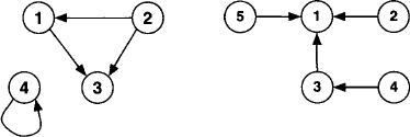
Example 2.1 Figure 2.1 displays two graphs: The left-hand graph G1 = (V1, E1) is specified by V1 = {1, 2, 3, 4} with E1 = {{1, 2}, {2, 3}, {3, 1}, {4}}. This graph is not connected, the neighbors of node 2 are ne(2) = {1, 3}, and the node set {1, 2, 3} forms a maximal clique. On the right, G2 = (V2, E2) is given by V2 = {1, 2, 3, 4, 5} and E2 = {{5, 1}, {1, 2}, {1, 3}, {3, 4}}. This graph is connected and since there are no cycles, it is a tree. The neighbors of node 1 are ne(1) = {2, 3, 5}, and the degree of G2 is deg(G2) = 3.
Figure 2.1 Undirected graphs.

In a directed graph G = (V, E) edges are ordered pairs of nodes E ![]() V × V. We thus refer to (i, j)
V × V. We thus refer to (i, j) ![]() E as the directed edge from node i to node j. A sequence of nodes (i0, i1, …, in) with (ik-, ik)
E as the directed edge from node i to node j. A sequence of nodes (i0, i1, …, in) with (ik-, ik) ![]() E for k = 1, …, n is called a path of length n from the source node i0 to the terminal node in. If i0 = in the path is again called a cycle. A directed graph is connected if for every pair of nodes i and j there exists either a path from i to j or from j to i. For every directed graph we find an associated undirected graph by ignoring all directions of the edges. We then say that a directed graph is a tree if its associated undirected graph is a tree. Moreover, if a directed graph is a tree and all edges are directed towards a selected node, then the graph is called a directed tree with the selected node as root node.
E for k = 1, …, n is called a path of length n from the source node i0 to the terminal node in. If i0 = in the path is again called a cycle. A directed graph is connected if for every pair of nodes i and j there exists either a path from i to j or from j to i. For every directed graph we find an associated undirected graph by ignoring all directions of the edges. We then say that a directed graph is a tree if its associated undirected graph is a tree. Moreover, if a directed graph is a tree and all edges are directed towards a selected node, then the graph is called a directed tree with the selected node as root node.
Example 2.2 Consider the two graphs in Figure 2.2. The left-hand graph G1 = (V1, E1) is specified by V1 = {1, 2, 3, 4} with E1 = {(1, 3), (2, 1), (2, 3), (4, 4)}. This graph is not connected. On the right, G2 = (V2, E2) is given by V2 = {1, 2, 3, 4, 5} and E2 = {(5, 1), (2, 1), (3, 1), (4, 3)}. This graph is a directed tree with root node 1.
Figure 2.2 Directed graphs.
Next, we consider directed or undirected graphs where each node possesses a label out of the powerset P(r) of a set of variables r. Thus, a labeled, undirected graph (V, E, λ, P(r)) is an undirected graph with a labeling function λ: V → P(r) that assigns a domain to each node. Such a graph is shown in Example 2.3.
Example 2.3 Figure2.3 shows a labeled graph (V, E, λ, V(r)) where V = {1, 2, 3, 4, 5}, E = {{5, 1}, {1, 2}, {1, 3}, {2, 4}, {4, 3}} and r = {A, B, C, D}. The labeling function λ is given by: λ(1) = λ(4) = {A, C, D}, λ(2) = {A, D}, λ(3) = {D} and λ(5) = {A, B}. Observe that node labels are not necessarily unique and therefore cannot replace the node numbering.
Figure 2.3 A labeled graph.

A hypergraph H = (V, S) is specified by a set of vertices or nodes V and a set of hyperedges S = {S1, …, Sn} which are subsets of V, i.e. Si ![]() V for i = 1, …, n. The primal graph of a hypergraph is an undirected graph (V, Ep) such that there is an edge {u, v}
V for i = 1, …, n. The primal graph of a hypergraph is an undirected graph (V, Ep) such that there is an edge {u, v} ![]() Ep for any two vertices u, v
Ep for any two vertices u, v ![]() V that appear in the same hyperedge,
V that appear in the same hyperedge,
![]()
The dual graph of a hypergraph is an undirected graph (S, Ed) that has a vertex for each hyperedge, and there is an edge {Si, Sj} ![]() Ed if the corresponding hyperedges share a common vertex, i.e. if Si
Ed if the corresponding hyperedges share a common vertex, i.e. if Si ![]() Sj ≠
Sj ≠ ![]() .
.
Example 2.4 Consider a hypergraph (V, S) with V = {1, 2, 3, 4, 5, 6} and S = {{1, 2, 3}, {3, 4, 5}, {1, 5, 6}}. Figure 2.4 shows a graphical representation of this hypergraph together with its associated primal and dual graphs.
Figure 2.4 The hypergraph and its associated primal and dual graphs of Example 2.4.

2.2 KNOWLEDGEBASES AND THEIR REPRESENTATION
Consider a valuation algebra ![]() for a set of variables r and a set of valuations {
for a set of variables r and a set of valuations {![]() 1, …,
1, …, ![]() n}
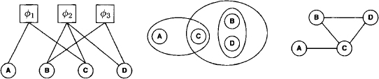
n} ![]() Φ. This valuation set stands for the available knowledge about some topic which constitutes the starting point of any deduction process. Accordingly, we refer to such a set as knowledgebase. It is often very helpful to represent knowledgebases graphically, since this uncovers a lot of hidden structure. There are numerous possibilities for this task, but most of them are somehow related to a particular instance. A general representation of knowledgebases are valuation networks: A valuation network (Shenoy, 1992b) is a graphical structure where variables are represented by circular nodes and valuations by rectangular nodes. Further, each valuation is connected with all variables of its domain. Valuation networks highlight the structure of a factorization and are therefore also called factor graphs (Kschischang et al., 2001) in the literature. Another general representation is given by the hypergraph H = (r, S) with S = {d(
Φ. This valuation set stands for the available knowledge about some topic which constitutes the starting point of any deduction process. Accordingly, we refer to such a set as knowledgebase. It is often very helpful to represent knowledgebases graphically, since this uncovers a lot of hidden structure. There are numerous possibilities for this task, but most of them are somehow related to a particular instance. A general representation of knowledgebases are valuation networks: A valuation network (Shenoy, 1992b) is a graphical structure where variables are represented by circular nodes and valuations by rectangular nodes. Further, each valuation is connected with all variables of its domain. Valuation networks highlight the structure of a factorization and are therefore also called factor graphs (Kschischang et al., 2001) in the literature. Another general representation is given by the hypergraph H = (r, S) with S = {d(![]() 1), …, d(
1), …, d(![]() n)} and its associated primal and dual graphs. These possibilities are also illustrated in Example 2.5.
n)} and its associated primal and dual graphs. These possibilities are also illustrated in Example 2.5.
Example 2.5 Figure 2.5 shows a valuation network, a hypergraph and its associated primal graph for the knowledgebase {![]() 1,
1, ![]() 2,
2, ![]() 3} with d(
3} with d(![]() 1) = {A, C}, d(
1) = {A, C}, d(![]() 2) = {B, C, D} and d(
2) = {B, C, D} and d(![]() 3) = {B, D}.
3) = {B, D}.
Figure 2.5 Representations for the knowledgebase in Example 2.5.
2.3 THE INFERENCE PROBLEM
The knowledgebase is the basic component of an inference problem. It represents all the available information that we may want to combine and project on the domains of interest. This is the statement of the following definition.
Definition 2.1 The task of computing
(2.2) ![]()
for a given knowledgebase {![]() 1, …,
1, …, ![]() n}
n} ![]() Φ and domains x = {x1, …, xs} where
Φ and domains x = {x1, …, xs} where ![]() is called an inference problem or a projection problem. The domains xi are called queries.
is called an inference problem or a projection problem. The domains xi are called queries.
The valuation ![]() resulting from the combination of all knowledgebase factors is often called joint valuation or objective function (Shenoy, 1996). Further, we refer to inference problems with |x| = 1 as single-query inference problems and we speak about multi-query inference problems if |x| > 1. For a better understanding of how different instances give rise to inference problems, we first touch upon a selection of typical and well-known fields of application that are based on the valuation algebra instances introduced in Chapter 1. Efficient algorithms for the solution of inference problems are discussed in Chapter 3 and 4. Here, we only focus on the identification of inference problems behind different applications.
resulting from the combination of all knowledgebase factors is often called joint valuation or objective function (Shenoy, 1996). Further, we refer to inference problems with |x| = 1 as single-query inference problems and we speak about multi-query inference problems if |x| > 1. For a better understanding of how different instances give rise to inference problems, we first touch upon a selection of typical and well-known fields of application that are based on the valuation algebra instances introduced in Chapter 1. Efficient algorithms for the solution of inference problems are discussed in Chapter 3 and 4. Here, we only focus on the identification of inference problems behind different applications.
![]() 2.1 Bayesian Networks
2.1 Bayesian Networks
A Bayesian network, as for instance in (Pearl, 1988), is a graphical representation of a joint probability distribution over a set of variables r = {X1, …, Xn}. The network itself is a directed, acyclic graph that reflects the conditional independencies among variables, which are associated with a node of the network. Each node contains a conditional probability table that quantifies the influence between variables. These tables can be considered as probability potentials, introduced as Instance 1.3. The joint probability distribution p of a Bayesian network is given by
(2.3) ![]()
where pa(Xi) denotes the parents of Xi in the network. If the set pa(Xi) is empty, the conditional probability becomes an ordinary probability distribution. Consider next a set q ![]() r called query variables and a set e
r called query variables and a set e ![]() r called evidence variables. The evaluation of a Bayesian network then consists in computing the posterior probability distribution for the query variables, given some observed values of the evidence variables. Such an observation corresponds to a tuple e
r called evidence variables. The evaluation of a Bayesian network then consists in computing the posterior probability distribution for the query variables, given some observed values of the evidence variables. Such an observation corresponds to a tuple e ![]() Ωe. Thus, if q
Ωe. Thus, if q ![]() Ωq denotes a query event, we want to compute the posterior probability p(q|e) defined as
Ωq denotes a query event, we want to compute the posterior probability p(q|e) defined as
(2.4) ![]()
To clarify how Bayesian networks give rise to inference problems, we consider an example from medical diagnostics (Lauritzen & Spiegelhalter, 1988).
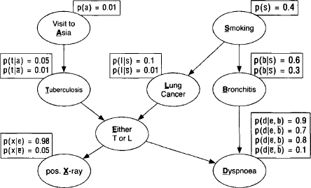
Shortness-of-breath (dyspnoea) may be due to tuberculosis, lung cancer or bronchitis, or none of them, or more than one of them. A recent visit to Asia increases the chances of tuberculosis, while smoking is known to be a risk factor for both lung cancer and bronchitis. The results of a single chest X-ray do not discriminate between lung cancer and tuberculosis, as neither does the presence or absence of dyspnoea. A patient presents himself at a chest clinic with dyspnoea and has recently visited Asia. Smoking history and chest X-ray are not yet available. The doctor wants to know the chance that this patient suffers from bronchitis.
Here, the query and evidence variables are easily identified: the query set q = {B} contains the variable standing for bronchitis, and the evidence variables e = {A, D} are dyspnoea and the recent visit to Asia. Figure 2.6 shows the Bayesian network of this example that reflects the dependencies among the involved variables r = {A, B, D, E, L, S, T, X}. All variables are assumed to be binary, e.g. the frame values ![]() refer to a smoking or nonsmoking patient respectively. Also, the Bayesian network shows the conditional probability tables that are associated with each node. These are the valuations of our example and can be modelled using the language of probability potentials. For example, we have
refer to a smoking or nonsmoking patient respectively. Also, the Bayesian network shows the conditional probability tables that are associated with each node. These are the valuations of our example and can be modelled using the language of probability potentials. For example, we have
Figure 2.6 The Bayesian network of the medical example. The bold-faced, underlined letters refer to the variable associated with the corresponding node.
Thus, we get a knowledgebase that consists of eight valuations (one probability potential for each node of the Bayesian network) and the joint valuation (joint probability mass function) is given by
(2.5) ![]()
To answer the query p(B|A, D) we therefore need to compute
![]()
and obtain our final answer by a last table lookup in p(B|A, D) to extract the entry that corresponds to the query and evidence event. To sum it up, evaluating the Bayesian network of the medical example requires to compute an inference problem with knowledgebase {p(A), p(T|A), …, p(D|E, B)} and query set {{A, B, D}, {A, D}}. In fact, it is sufficient to compute the query {A, B, D} because p(A, D) can easily be obtained from this result by one last projection
(2.6) ![]()
![]() 2.2 Query Answering in Relational Databases
2.2 Query Answering in Relational Databases
The procedure of query answering in a relational database is another example of an inference problem. The knowledgebase is a set of database tables that are elements of the valuation algebra of relations introduced as Instance 1.2. The inference problem then computes the natural join of all relations in the knowledgebase and projects the result on the attributes of interest. However, it is important to note that the selection operator, which is integral part of every relational database system, does not directly have a counterpart in the valuation algebra framework. Nevertheless, there are techniques that allow embedding selections. A particular simple but limited possibility is to transform selections into relations themselves that are then added to the knowledgebase. The advantage of this method is that we stay on a generic level and do not need to care about selections during the computations. On the other hand, transforming selections may create relations of infinite cardinality if special queries over attributes with infinite frames are involved. In such cases, more complex techniques are required that extend the definition of inference problems and treat selections explicitly. We refer to (Schneuwly, 2007) for a detailed discussion of selection enabled local computation. In the following (self-explanatory) example we focus on the first method and convert selections into relations.
Thus, we get a knowledgebase of five relations {r1, …, r5}. Let us further assume the following database query:
Find all students with grade A or B in a lecture of professor Einstein.
This gives us the single query for the inference problem {Student}. In addition, it contains two selections which correspond to the following new relations:
Thus, we finally derive the inference problem
![]()
![]() 2.3 Reasoning with Mass Functions
2.3 Reasoning with Mass Functions
Mass functions correspond to the formalism of set potentials introduced as Instance 1.4 with an additional condition of normalization. They are used to represent knowledge in the Dempster-Shafer theory of evidence (Shafer, 1976) and provide similar reasoning facilities as Bayesian networks, but with different semantics as pointed out in (Smets & Kennes, 1994; Kohlas & Monney, 1995). It will be shown in Section 4.7 that normalization in the context of valuation algebras can be treated on a generic level. We therefore neglect normalization and directly use set potentials for reasoning with mass functions in the subsequent example. Normalized set potentials will later be introduced in Instance D.9. The following imaginary example has been proposed by (Shafer, 1982):
Imagine a disorder called ploxoma which comprises two distinct diseases: θ1 called virulent ploxoma, which is invariably fatal, and θ2 called ordinary ploxoma, which varies in severity and can be treated. Virulent ploxoma can be identified unequivocally at the time of a victim’s death, but the only way to distinguish between the two diseases in their early stages is a blood test with three possible outcomes X1, X2 and X3. The following evidence is available:
1. Blood tests of a large number of patients dying of virulent ploxoma showed the outcomes X1, X2 and X3 occurring 20, 20 and 60 per cent of the time, respectively.
2. A study of patients whose ploxoma had continued so long as to be almost certainly ordinary ploxoma showed outcome X1 to occur 85 per cent of the time and outcomes X2 and X3 to occur 15 per cent of the time. (The study was made before methods for distinguishing between X2 and X3 were perfected.) There is some question whether the patients in the study represent a fair sample of the population of ordinary ploxoma victims, but experts feel fairly confident (say 75 per cent) that the criteria by which patients were selected for the study should not affect the distribution of test outcomes.
3. It seems that most people who seek medical help for ploxoma are suffering from ordinary ploxoma. There have been no careful statistical studies, but physicians are convinced that only 5–15 percent of ploxoma patients suffer from virulent ploxoma.
This story introduces the variables D for the disease with the possible values {θ1,θ2} and T for the test result taking values from {X1,X2,X3}. (Shafer, 1982) comes up with a systematic disquisition on how to translate this evidence into mass functions in a meaningful manner. Here, we do not want to enter into this discussion and directly give the corresponding knowledgebase factors. Instead, we focus on the fact that reasoning with mass functions again amounts to the solution of an inference problem.
The mass function m1 derived from the first statement is:
For example, our belief that the blood test returns X3 for a patient with virulent ploxoma θ1 is 0.6. This mass function does not give any evidence about the test outcome with disease θ2. The second factor m2 is:
For example, in case of ordinary ploxoma θ2 the test outcome is X1 in 85 per cent of all cases. This value is scaled with the expert’s confidence of 0.75. There are 25 per cent of cases where the test tells us nothing whatsoever. Finally, the third mass function m3 is:
For example, the belief that a patient, who seeks medical help for ploxoma, suffers from θ2 is 0.85. Here, the value 0.1 signifies that it is not always possible to distinguish properly between the two diseases.
Let us now assume that we are interested in the reliability of the test result. In other words, we want to compute the belief held in the presence of either θ1 or θ2 given that the test result is for example X1. Similar to Bayesian networks, this is achieved by adding the observation mo to the knowledgebase which expresses that the test result is X1:
![]()
Thus, we obtain the belief for the presence of either virulent or ordinary ploxoma by solving the following computational task:
![]()
This is clearly an inference problem with knowledgebase {m1,m2,m3,mo} and query {T}. Although this example with only 4 knowledgebase factors, one query and two variables seems easily manageable, it is already a respectable effort to solve it by hand. We therefore refer to (Blau et al., 1994) where these computations are executed and commented.
![]() 2.4 Satisfiability
2.4 Satisfiability
Let us consider a digital circuit build from AND, OR and XOR gates which are connected as shown in Figure 2.7. Each gate generates an output value from two input values according to the following tables:
Figure 2.7 A digital circuit of a binary adder.

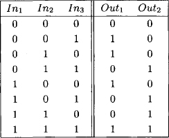
This particular circuit is called full adder since it computes the binary addition of the three input values as shown in Figure 2.8. The value Out1 corresponds to the carry-over bit.
Figure 2.8 The result table of a full adder circuit.
From the adder circuit in Figure 2.7, we extract the following five Boolean functions that constitute our knowledgebase {![]() 1, …,
1, …, ![]() 5}:
5}:
Now, imagine the following situation: we insert the values In1 = 0, In2 = 0 and In3 = 0 into the above adder circuit and observe Out1 = 1 and Out2 = 1. A quick glance on Figure 2.8 confirms that this result can only be produced by a faulty adder component. Fortunately, we are supplied with a voltage meter to query the actual values of each line V1 to V3, which can be used to locate the fault. However, this requires that the correct line values for the particular input are known which cannot be deduced from the above tables. We therefore add the three Boolean function ![]() 6: In1 = 0,
6: In1 = 0, ![]() 7: In2 = 0 and
7: In2 = 0 and ![]() 8: In3 = 0 to our knowledgebase and compute the inference problem with query {V1, V2, V3}:
8: In3 = 0 to our knowledgebase and compute the inference problem with query {V1, V2, V3}:
![]()
Here, we compute in the valuation algebra of Boolean functions introduced in Instance 1.1. Computing this query gives V1 = 1, V2 = 0 and V3 = 0 as the correct line values which now makes the physical monitoring process possible. Alternatively, we may also deduce the correct input or output values from partial observations: If we for example know that ![]() 9: In3 = 0 and
9: In3 = 0 and ![]() 10: Out2 = 0, solving the inference problem
10: Out2 = 0, solving the inference problem
![]()
gives In1 = 1, In2 = Out1 = 0. Clearly, it would have been possible to extract this result from Figure 2.8 directly, but building this table becomes quickly intractable even for an only slightly larger circuit. How such larger adder circuits are constructed from the one-bid-adder is shown in Figure 2.9.
Figure 2.9 Connecting two 1-bit-adders produces a 2-bit-adder.

This example of an inference problem is a very classical application of constraint programming, and many similar applications can be found in the corresponding literature. For example, we refer to (Apt, 2003) for a collection of constraint satisfaction problems. However, let us point out that the various constraint formalisms indeed represent an important class of valuation algebras, but there are many further instances beyond classical constraints. We will discuss different constraint formalism in Chapter 5 and also show that they all instantiate the valuation algebra framework.
![]() 2.5 Hadamard Transforms
2.5 Hadamard Transforms
The Hadamard transform (Beauchamp, 1984; Gonzalez & Woods, 2006) is an essential part of many applications that incorporate error correcting codes, random number generation or image and video compression. The unnormalized variant of a Hadamard transform uses a 2m × 2m Hadamard matrix Hm that is defined recursively by the so-called Sylvester construction:
![]()
For instance, we obtain for m = 3,
Hadamard matrices have many interesting properties: they are symmetric, orthogonal, self–inverting up to a constant and any two rows differ in exactly 2m-1 positions. The columns of a Hadamard matrix are called Walsh functions. Thus, if we multiply Hadamard matrix with a real-valued vector v, we obtain a transformation of this vector into a superposition of Walsh functions which constitutes the Hadamard transform. For illustration, assume three binary variables X1 to X3 and a function ![]() . This function is completely determined by its values vi for i = 0, …, 7. We then obtain for its Hadamard transform,
. This function is completely determined by its values vi for i = 0, …, 7. We then obtain for its Hadamard transform,
An alternative way to compute this Hadamard transform bears on a duplication of variables (Aji & McEliece, 2000). We introduce the binary variables Y1 to Y3 which give a binary representation of the line number in the Hadamard matrix. Then, the same computational task is expressed by the formula
![]()
The reader may easily convince himself of the equivalence between the two computational tasks. In this alternative representation, we discover a sum over a multiplication of four discrete functions taking real values or, in other words, an inference problem over the valuation algebra of arithmetic potentials, where the knowledgebase consists of the four discrete functions, and the single query is {Y1,Y2,Y3}. Thus, we could alternatively write for the Hadamard transform:
(2.7) ![]()
which is reduced to the solution of a singe-query inference problem.
![]() 2.6 Discrete Fourier and Cosine Transforms
2.6 Discrete Fourier and Cosine Transforms
Our last example of an inference problem comes from signal processing. For a positive integer ![]() we consider a function
we consider a function ![]() that represents a sampled signal, i.e. the value
that represents a sampled signal, i.e. the value ![]() corresponds to the signal value at time 0 ≤ x ≤ N - 1. Thus, the input signal is usually said to be in the time domain although any kind of sampled data may serve as input. The complex, discrete Fourier transform then changes the N point input signal into two N point output signals which contain the amplitudes of the component sine and cosine waves. It is given by
corresponds to the signal value at time 0 ≤ x ≤ N - 1. Thus, the input signal is usually said to be in the time domain although any kind of sampled data may serve as input. The complex, discrete Fourier transform then changes the N point input signal into two N point output signals which contain the amplitudes of the component sine and cosine waves. It is given by
for 0 ≤ y ≤ N - 1. Accordingly, F is usually said to be in frequency domain. The discrete Fourier transform has many important applications as for example in audio and image processing or data compression. We refer to (Smith, 1999) for a survey of different applications and for a more detailed mathematical background. Figure 2.10 gives an illustration of the discrete Fourier transform.
Figure 2.10 Input and output of a complex, discrete Fourier transform.

The following procedure of transforming a discrete Fourier transform into an inference problem was proposed by (Aji, 1999) and (Aji & McEliece, 2000). Let us take N = 2m for some ![]() and write x and y in binary representation:
and write x and y in binary representation:
with Xj,Yl ![]() {0,1}. This corresponds to an encoding of x and y into binary configurations x = (X0, …, Xm-1) and y = (Y0, …, Ym-1). Observe that we may consider the components X1 and Y1 as new variables of this system (therefore the notation as capital letters). The product xy then gives
{0,1}. This corresponds to an encoding of x and y into binary configurations x = (X0, …, Xm-1) and y = (Y0, …, Ym-1). Observe that we may consider the components X1 and Y1 as new variables of this system (therefore the notation as capital letters). The product xy then gives
![]()
We insert this encoding into equation (2.8) and obtain
The last equality follows since the exponential factors become unity when j + l ≥ m. Introducing the short-hand notation
![]()
we obtain for the equation (2.8):
![]()
This is an inference problem over the valuation algebra of (complex) arithmetic potentials. All variables r = {N0, …, Nm-1, K0, …, Km-1} take values from {0,1} and the discrete functions f and ej,l map binary configurations to complex values. The knowledgebase is therefore given by
![]()
and the query of the inference problem is {K0, …, Km-1}. Thus, we could alternatively express the computational task of a discrete Fourier transform as
(2.9) ![]()
Observe that the inference problem behind the discrete Fourier transform has been uncovered by the artificial introduction of variables that manifests itself in the ej,l knowledgebase factors. This knowledgebase has a very particular structure as shown by the board in Figure 2.11. For m = 8, each cell of this board corresponds to one factor ej,l with j identifying the row and l the column. Observe, however, that only the shaded cells refer to functions contained in the knowledgebase. As it will be shown in Section 3.11, this sparse structure of the knowledgebase enables the efficient solution of this inference problems by the local computation procedures introduced in the next chapter.
Figure 2.11 Illustration of the ej,l functions in the inference problem of the discrete Fourier transform with m = 8. Index j identifies the row, and index l the column. The shaded cells refer to the functions contained in the knowledgebase.

The same technique of introducing binary variables can be applied to other discrete, linear transforms such as the discrete cosine transform which for example plays an important role in the JPEG image compression scheme. See Exercise B.1.
2.4 CONCLUSION
Sets of valuations are called knowledgebases and represent the available knowledge at the beginning of an inference process. There are several possibilities for visualizing knowledgebases and their internal structure. Most important are valuation networks, hypergraphs and their associated primal and dual graphs. The second ingredient of an inference task is the query set. According to the number of queries, we distinguish between single-query inference problems and multi-query inference problems. Inference problems state the main computational interest in valuation algebras. They require combining all available information from the knowledgebase and projecting the result afterwards on the elements of the query set. Depending on the underlying valuation algebra inference problems adopt very different meanings. Examples of applications that attribute to the solution of inference problems are reasoning tasks in Bayesian and belief networks, query answering in relational databases, constraint satisfaction and discrete Fourier or Hadamard transforms.
PROBLEM SETS AND EXERCISES
B.1* The discrete cosine transform of a signal f is defined by
(2.10) 
Exploit the binary representation of x and y and the identity
![]()
to transform this formula into two inference problems over the valuation algebra of arithmetic potentials. A similar technique has been applied for the discrete Fourier transform in Instance 2.6. Compare the knowledgebase factors, their domains and the query sets of the two inference problems and also with the inference problem of the discrete Fourier transform.
B.2* Assume that we want to determine the exact weight of an object. It is clear that the result of a weighting process always includes an unknown error term. Using ![]() different balances, we thus obtain n different observations xi = m + ωi for i = 1, …, n, where m refers to the object weight and ωi to the error term. We further assume that the errors of the different devices are mutually independent and normally distributed with mean value 0 and variance σi2. Rewriting the above equation as m = xi - ωi, we obtain a Gaussian potential
different balances, we thus obtain n different observations xi = m + ωi for i = 1, …, n, where m refers to the object weight and ωi to the error term. We further assume that the errors of the different devices are mutually independent and normally distributed with mean value 0 and variance σi2. Rewriting the above equation as m = xi - ωi, we obtain a Gaussian potential ![]() for each measurement. For simplicity, assume m = 2 and determine the combined potential
for each measurement. For simplicity, assume m = 2 and determine the combined potential ![]() by the combination rule in Instance 1.6. Then, by choosing σ1 = σ2 (balances of the same type), show that the object weight m corresponds to the arithmetic mean of the observed values. These calculations mirror the solution of a (trivial) projection problem where the domain of the objective function
by the combination rule in Instance 1.6. Then, by choosing σ1 = σ2 (balances of the same type), show that the object weight m corresponds to the arithmetic mean of the observed values. These calculations mirror the solution of a (trivial) projection problem where the domain of the objective function ![]() consists of only one variable. A more comprehensive example will be given in Section 10.1.
consists of only one variable. A more comprehensive example will be given in Section 10.1.
B.3* We proved in Exercise A.2 that possibility potentials form a valuation algebra. In fact, this corresponds to the valuation algebra of probability potentials with addition replaced by maximization. Apply this algebra to the Bayesian network of Instance 2.1 and show that the projection problem with empty domain identifies the value of the most probable configuration in the objective function.
B.4* Figure 2.12 shows a representation of a stochastic process called hidden Markov chain. The random variables Xk refer to the state of the process at time k = 1, …, n and are subject to a known transition probability p(Xk+1|Xk). Further, we assume that a prior probability p(X0) for the first variable X]0 is given. However, the states of the hidden Markov chain cannot be observed from the outside. Instead, a second random process with variables Yk generates an observable state at each point in time that only depends on the real but hidden state Xk with a known probability p(Yk|Xk). For a fixed k ≥ 0, a hidden Markov chain is a particular Bayesian network. There are three computational problems related to hidden Markov chains:
Figure 2.12 A hidden Markov chain.
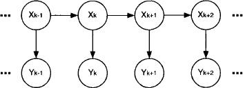
- Filtering: Given an observed sequence of states y1, … yk, determine the probability of the hidden state Xk by computing p(Xk|Y1 = y1, …, Yk = yk).
- Prediction: Given an observed sequence of states y1, … yk and n > 1, determine the probability of the hidden state at some point k + n in the future by computing p(Xk+n|Y1 = y1, …., Yk = yk). This corresponds to repeated filtering without new observations.
- Smoothing: Given an observed sequence of states y1, … yk and 1 ≥ n ≥ k, determine the probability of the hidden state at some point k - n in the past by computing p(Xk-n|Y1 = y1, …, Yk = yk).
Show that the computational tasks of filtering, prediction and smoothing in hidden Markov chains can be expressed by projection problems with different query sets in the valuation algebra of probability potentials. How does the meanings of these projection problems change when the valuation algebra of possibility potentials from Exercise A.2 is used? Hidden Markov chains and other stochastic processes will be reconsidered in Chapter 10.