CHAPTER 2
COMMON APPROACHES FOR MEASURING AGREEMENT
2.1 PREVIEW
The notion of agreement between two methods of measurement of a continuous response variable was introduced in Section 1.5. This chapter describes some common measures of agreement and discusses approaches for agreement evaluation based on those measures. The specific ones considered include concordance correlation coefficient, total deviation index, and limits of agreement. These are used throughout the book.
2.2 INTRODUCTION
As in Chapter 1, we use (Y1, Y2) to denote a pair of measurements by the two methods on a randomly selected subject from a population of interest. The pair follows a continuous bivariate distribution with mean (µ1, µ2), variance ![]() , covariance σ12, and correlation ρ. Let D = Y1 − Y2 denote the difference in measurements. It follows a continuous distribution with mean ξ = µ1 − µ2 and variance
, covariance σ12, and correlation ρ. Let D = Y1 − Y2 denote the difference in measurements. It follows a continuous distribution with mean ξ = µ1 − µ2 and variance ![]() . The distributions of Y1, Y2, and D need not be normal, although we often make such an assumption for inference purposes.
. The distributions of Y1, Y2, and D need not be normal, although we often make such an assumption for inference purposes.
From Section 1.5, when the methods have perfect agreement, that is, P (Y1 = Y2) = 1, the bivariate distribution of Y1 and Y2 is concentrated on the 45◦ line. The deviation from this ideal are quantified by agreement measures, which are functions of parameters of the bivariate distribution. Different measures quantify the deviation differently. For example, some are based on the joint properties of Y1 and Y2 while others are based directly on the difference. Likewise, some are defined in terms of moments of a distribution and others are defined in terms of quantiles. Nevertheless, the agreement measures generally tend to be scalar quantities, with either small or large values implying good agreement between the methods. Perfect agreement is implied by specific boundary values of the measures. We now define some commonly used measures and explain how they are used to evaluate agreement. The estimation of these measures is discussed in subsequent chapters.
2.3 MEAN SQUARED DEVIATION
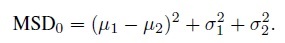
The mean squared deviation (MSD) is based on the difference D. It is defined as
 (2.1)
(2.1)where the second equality follows from the fact that
 (2.2)
(2.2)This measure quantifies the average size of the squared differences in measurements. Clearly, MSD ≥ 0, with small values implying good agreement. It depends on the parameters of the bivariate distribution of (Y1, Y2) through the mean ξ and variance τ2 of D. For this measure to be small, both |ξ| and τ must be small. Perfect agreement corresponds to MSD = 0.
To evaluate agreement using MSD, we can construct its upper confidence bound U from the data and judge whether the extent of agreement represented by the value U for MSD may be considered acceptable (Section 1.11). Alternatively, letting φ denote the MSD and φ0 denote a specified threshold below which MSD is considered small enough for sufficient agreement, we can test the agreement hypotheses (1.14). Sufficient agreement is inferred if U < φ0. However, judging whether a given value of MSD represents acceptable agreement is generally a difficult task for practitioners. The same holds for specifying the cutoff φ0. This difficulty in interpretation of an MSD limits its practical utility. But due to its intuitively appealing properties, MSD often serves as a starting point for defining other measures of agreement.
The notion of MSD can be generalized to get an entire class of MSD-like measures. For this, we replace D2 in (2.1) with a distance function g(Y1, Y2) to get
 (2.3)
(2.3)as the generalized measure. In particular, taking g(y1, y2) = (y1 − y2)2, the squared distance function, leads to the usual MSD. Additional choices for g, for example, g(y1, y2) = |y1 − y2|, the absolute distance function, lead to other MSD-like measures (see Bibliographic Note).
2.4 CONCORDANCE CORRELATION COEFFICIENT
To define the concordance correlation coefficient (CCC), we start with the MSD measure and rescale it to lie between −1 to 1. Formally,
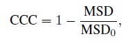 (2.4)
(2.4)where MSD0 is the MSD value assuming Y1 and Y2 are independent. Under independence, the covariance σ12 = 0, implying
Therefore, it follows from (2.2) that
 (2.5)
(2.5)Substituting (2.1) and (2.5) in (2.4) and simplifying, we get the CCC as (Exercise 2.1)
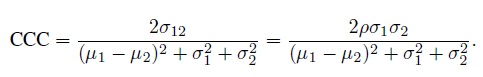 (2.6)
(2.6)This measure is a function of the first- and second-order moments of (Y1, Y2).
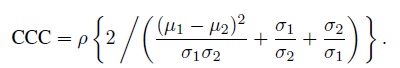
An alternative form for CCC is obtained by dividing both numerator and denominator in (2.6) by σ1 σ2 to get
 (2.7)
(2.7)This form decomposes CCC as a product of two factors. The first factor is simply the correlation ρ, which measures how tightly concentrated the bivariate distribution is around a straight line. The second factor measures how close the two marginal distributions are with respect to their means and variances, and itself is made up of two components. The first component measures squared difference in the means standardized by the product of the standard deviations. The second component, consisting of the sum of ratios of the standard deviations, measures difference in the standard deviations. It is smallest (with a value of 2) when the standard deviations are equal. Taken together, the second factor lies between zero and one, with the value of one corresponding to {µ1 = µ2, σ1 = σ2}. Thus, it shrinks the first factor ρ towards zero.
The CCC has the following properties (Exercise 2.1):
- CCC has the same sign as ρ.
- 0 ≤ |CCC| ≤ |ρ| ≤ 1.
- CCC = ρ ⇔ {µ1 = µ2, σ1 = σ2}.
- |CCC| = second factor in (2.7) ⇔ |ρ| = 1.
- CCC = 0 ⇔ ρ = 0, implying uncorrelated measurements.
- CCC = 1 ⇔ {µ1 = µ2, σ1 = σ2, ρ = 1}, implying perfect agreement.
- CCC = −1 ⇔ {µ1 = µ2, σ1 = σ2, ρ = −1}, implying perfect negative agreement, that is, P (Y1 = −Y2) = 1.
Clearly, large positive values of CCC indicate good agreement. Since the CCC cannot exceed ρ in absolute value, a weak correlation always implies a low agreement. The converse, however, is not true in general because CCC may be small even when ρ = 1 due to a large value for the denominator of the second factor in (2.7), see (iv) above. Although the CCC may be negative, it is rarely so in practice because two methods designed to measure the same underlying quantity tend to be positively correlated. The interpretation of a negative CCC is problematic in view of the fact that a larger difference in the means of the methods, implying worse agreement, leads to a higher value for the CCC (Exercise 2.2).
We may think of MSD0 in (2.5) as a measure of chance agreement in that it reflects the extent of agreement expected when the measurements from the two methods are independent. Therefore, from (2.4), the CCC may be viewed as a chance-corrected measure, reflecting the extent of agreement in excess of what is expected by chance alone. Such measures have a history dating back to at least 1960 when the kappa statistic a popular chance-corrected measure of agreement for categorical data—became available. Agreement measures for categorical data are presented in Chapter 12, where we will explore this connection further.
The CCC has an important limitation that needs to be considered while interpreting it. Just like any correlation-type measure, CCC is highly sensitive to the between-subject variation in the data (Section 1.6.2). If this variation is large, the estimated CCC may be high regardless of how large or small the differences in measurements are. The converse would be true if this variation is small. Exercise 2.3 illustrates this point with two datasets that have identical differences in measurements, and hence exhibit the same level of agreement in a sense, but have substantially different estimates of CCC simply because one dataset is more heterogeneous than the other. Thus, it follows that the CCCs estimated from two different datasets are not comparable unless the data have similar levels of heterogeneity. This behavior of CCC can be explained by its expression in (2.7). Therein the CCC is shown as a product of correlation ρ, which from (1.9) in Section 1.6.2 is known to be sensitive to heterogeneity of true values expressed through ![]() , and a term that is relatively unaffected by
, and a term that is relatively unaffected by ![]() (see Exercise 2.3).
(see Exercise 2.3).
As large (positive) values for CCC imply good agreement, we can evaluate agreement based on CCC by constructing its lower confidence bound L from the data, and assessing whether the value L for CCC represents acceptable agreement. Alternatively, letting φ denote the CCC and φ0 denote a threshold above which the CCC represents acceptable agreement, we can test the agreement hypotheses (1.15). Sufficient agreement is inferred if L > φ0. In the light of the drawback of CCC, this assessment should be cognizant of the between-subject variation in the data. An assessment based on arbitrary cutoffs, such as “high agreement if L exceeds 0.90,” may be misleading and therefore should be avoided. Besides, any analysis based on CCC should be supplemented by an analysis based on another measure that is not as sensitive to the between-subject variation as the CCC. Examples are provided in subsequent chapters.
Note that the assumption of independence is not necessary to define the MSD0 in (2.4) and hence the CCC. The weaker assumption of uncorrelated Y1 and Y2 leads to the same expression. However, the independence assumption is useful in generalizing CCC to a class of CCC-like measures. The generalization is accomplished by simply replacing the MSD in (2.4) by its generalized version (2.3), yielding
 (2.8)
(2.8)as the generalized CCC. Here g is a distance function and E0 denotes expectation under the assumption that Y1 and Y2 are independent. Taking g(y1, y2) = (y1 − y2)2 in (2.8) gives the usual CCC. A version that is more robust to outliers in the data can be obtained by taking g(y1, y2) = |y1 − y2| (see Bibliographic Note). The generalization (2.8) also allows unifying the treatment of chance-corrected measures for both continuous and categorical data in a single framework (see Chapter 12).
2.5 A DIGRESSION: TOLERANCE AND PREDICTION INTERVALS
In this section, we briefly digress to present an overview of tolerance and prediction intervals. These intervals provide interval estimates of a range containing a specified proportion of the population being sampled. They play a prominent role in agreement evaluation and are used in subsequent sections. They are distinct from a confidence interval, which provides an interval estimate for a population parameter.
2.5.1 Definitions
Let X denote a continuous random variable, and fX and FX be its probability density function (pdf) and cumulative distribution function (cdf), respectively. In practice, we will have some data from the population of X, but to define the intervals there is no need to make assumptions about the data design. Let I = (L, U) be a random interval computed from the sample data. Define the probability content of the interval I as
 (2.9)
(2.9)This probability content, also called the coverage of the interval I, is a random variable representing the proportion of the population of X values contained in I. It can also be interpreted as the proportion of all future observations from the population of X, sampled independently of the observed data, that is contained in I.
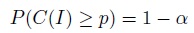
Definition (Tolerance interval) A random interval I = (L, U) is a tolerance interval containing 100p% of the distribution of X with 100(1 − α)% confidence if
 (2.10)
where C(I) is the probability content given by (2.9).
The probability in (2.10) is computed using the sampling distribution of the data. The endpoints of a tolerance interval are called tolerance limits. There are two equivalent interpretations of this interval. One, it contains at least p proportion of the sampled population with confidence 1 − α. Two, it covers at least p proportion of all future observations from the population of X with confidence 1 − α.
Let Xf denote a single future observation from the population of X, sampled independently of the observed data. By definition, X and Xf are identically distributed.
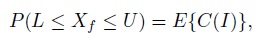
Definition (Prediction interval) A random interval I = (L, U) is a prediction interval for X with 100p% confidence if
 (2.11)
The probability in (2.11) is computed using the joint distribution of the sample data and Xf. The endpoints of a prediction interval are called prediction limits. There are two equivalent interpretations of a prediction interval as well. The first follows directly from its definition: the interval contains a single future observation from the sampled population with confidence p. The second is due to the fact that
 (2.12)
where the expectation on the right is with respect to the sampling distribution of the data (Exercise 2.4). Thus, a 100p% prediction interval contains, on average, at least p proportion of the sampled population.
A comparison of (2.10), (2.11), and (2.12) shows that, for a specified p, the probability content of a prediction interval is at least p on average, whereas that of a tolerance interval is at least p with probability 1 − α. Since 1 − α in practice is close to 1, we may say that what a prediction interval does merely on average is done by a tolerance interval with a large probability 1 − α. As a result, a tolerance interval is generally wider than the corresponding prediction interval. These intervals are said to be conservative if the probabilities in their definitions (2.10) and (2.11) are strictly greater than the specified lower bounds.
Prediction and tolerance intervals are not unique. Two such intervals may contain the same overall proportion of the population, but the specific regions they contain may be located in different parts of the distribution, for example, in the center or in the tails. In particular, the intervals can be one-sided (if either L = − ∞ or U = ∞) or two-sided. Here we focus only on two-sided intervals.
2.5.2 Normally Distributed Data
We now describe a methodology for computing two-sided tolerance and prediction intervals that contain 100p% of the population of x, assuming that X ∼ N1 (µ, σ2) with both parameters unknown. For simplicity, we also assume that the data consist of a random sample X1,..., Xn from this population. The methodology can be generalized to handle data from more complex designs. We also focus on the intervals of the form
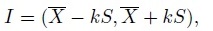 (2.13)
where ![]() is the sample mean,
is the sample mean, ![]() is the sample variance, and k—a positive quantity—is an appropriately chosen factor. The probability content of this interval can be expressed as
is the sample variance, and k—a positive quantity—is an appropriately chosen factor. The probability content of this interval can be expressed as

where Φ is the cdf of a N1 (0, 1) distribution. Note that C(I) is a function of k as well as unknown (µ, σ2) and their estimates. But it is a pivotal quantity whose distribution is completely known and is free of the unknown parameters.
By definition, the factor k for a tolerance interval is obtained by solving the equation
for k. Let ktol = ktol (n, p, α) be the solution, implying
 (2.14)
forms a 100p% tolerance interval with 100(1 − α)% confidence. The factor ktol is not available in a closed form and must be computed numerically. A good approximation is given by (see Bibliographic Note)
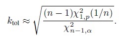 (2.15)
It is worth noting that the interval (2.14), although centered at ![]() , does not guarantee to contain the interval
, does not guarantee to contain the interval
 (2.16)
holding the middle 100p% of the population. The interval (2.14) merely guarantees to contain a two-sided region of the distribution that holds 100p% of the population. It is possible to compute the factor k so that the resulting interval does contain the middle 100p% of the population (Exercise 2.7).
To determine the factor k for a prediction interval, first we see that (Exercise 2.5)
 (2.17)
where the random variable Tν follows a t distribution with ν degrees of freedom. Next, we set (2.17) equal to p and explicitly solve for k. This leads to a 100p% prediction interval of the form (Exercise 2.5)
 (2.18)
2.6 LIN’S PROBABILITY CRITERION AND BLAND-ALTMAN CRITERION
In this section, we present an intuitively appealing premise that lies at the heart of three approaches for agreement evaluation that will be described in the next two sections. These are limits of agreement, total deviation index, and coverage probability. The premise is that two measurement methods may be considered to have sufficient agreement if a large proportion of their differences is small. To state the underlying criterion more precisely, let p be a specified large proportion, and ± δ, for δ > 0, be a specified acceptable margin for the differences in that a difference falling within ± δ is acceptably small (or practically insignificant). The choices of p and δ are subjective and depend on the application. The criterion can now be stated as follows: the two methods have sufficient agreement if
 (2.19)
We call it the Lin’s probability criterion after L. I. Lin, who developed the total deviation index and was involved in the development of the coverage probability approach. It simply asks for more than 100p% of the distribution of D to be contained within the acceptable margin, without being specific about the location of the differences. A more stringent variant of it requires the middle 100p% of the distribution of D to be contained within ± δ. We refer to it as the Bland-Altman criterion after J. M. Bland and D. G. Altman, who developed the limits of agreement approach. This criterion may be appropriate when D has a symmetric distribution. For example, when D ∼ N1 (ξ, τ2), from (2.16), the criterion requires
 (2.20)
If two measurement methods satisfy the Bland-Altman criterion, then they necessarily satisfy the Lin’s probability criterion, but the converse is not true.
To evaluate agreement using these criteria, three statistical approaches seem natural. The first approach is to compute a tolerance interval for D and compare it with the margin ± δ. Sufficient agreement can be inferred if the interval falls within the margin. As see in Section 2.5, the interval guarantees to contain at least 100p% of differences in all future measurements with 100(1 − α)% confidence. Therefore, for sufficient agreement, this decision rule requires more than 100p% of differences in measurements to be acceptable with 100(1 − α)% confidence. This rule may be useful for a regulator in charge of approving measurement methods for interchangeable use, who needs to ensure that the differences in a large proportion of all future measurements from the two methods are acceptably small.
The second approach is to perform a test of agreement hypotheses of the form (1.13) where either the Lin’s probability criterion (2.19) or the Bland-Altman criterion (2.20) forms the alternative hypothesis. The former is pursued later in Section 2.8, where we will also see that testing the relevant hypotheses is equivalent to employing a tolerance interval. Exercise 2.9 provides an example of the latter.
The third approach is to compute a prediction interval for D and compare it with the margin ± δ. It may seem that sufficient agreement can be inferred if the interval falls within the margin. However, from Section 2.5, a prediction interval for D merely guarantees to contain the difference in a single future measurement from the two methods with 100p% confidence. Therefore, this decision rule is only useful for an individual who just needs to make a single measurement and is trying to decide which method to use. It is not useful if the individual desires to select a method and use it for making several measurements because the prediction interval offers no guarantees for containing more than one future difference. Thus, a prediction interval is of limited value in the usual agreement evaluation problems where one would like to infer whether two methods agree sufficiently well for interchangeable use of the methods, not just for making a single future measurement, but for making at least a large proportion of all future measurements. When both p and 1 − α are close to 1, as is typically the case, a prediction interval is completely contained within the corresponding tolerance interval. As a result, whenever the tolerance interval lies within the margin, so does the prediction interval.
2.7 LIMITS OF AGREEMENT
2.7.1 The Approach
The limits of agreement approach is presently the most popular approach for agreement evaluation in biomedical disciplines. It works with the difference D, and assumes that D ∼ N1 (ξ, τ2). Then, it takes the interval (ξ − 1.96τ, ξ + 1.96 τ) covering the middle 95% of the population of D as the measure of agreement. The endpoints of this interval represent the 2.5th and the 97.5th percentiles of D. This population interval is estimated by the interval ![]() , whose endpoints are called the 95% limits of agreement. In the case of paired measurements data, the estimator
, whose endpoints are called the 95% limits of agreement. In the case of paired measurements data, the estimator ![]() of (ξ, τ2) is taken as
of (ξ, τ2) is taken as ![]() , where the sample mean D and the sample variance
, where the sample mean D and the sample variance ![]() of the differences are given by (1.17).
of the differences are given by (1.17).
If the limits of agreement fall within a specified margin ± δ, that is,
 (2.21)
the methods are inferred to have sufficient agreement for interchangeable use. Although δ is recommended to be specified in advance, it is rarely done so in practice. Instead, the practitioners typically evaluate agreement by judging whether or not the endpoints of the region ![]() may be considered unacceptably large.
may be considered unacceptably large.
An integral component of this approach is the use of the Bland-Altman plot (Section 1.13) to display the data. Further, to provide a graphical summary of the results, three horizontal lines—one for the mean difference ![]() and one each for the two limits—are superimposed on this plot. It is also necessary to verify the normality assumption for D because the 95% limits may not estimate a 95% population range if the distribution is not normal.
and one each for the two limits—are superimposed on this plot. It is also necessary to verify the normality assumption for D because the 95% limits may not estimate a 95% population range if the distribution is not normal.
Although this approach uses 95% limits by default, the limits for some other specified large percentage, say 100p%, may be used as well. The general approach takes the interval ![]() covering the middle 100p% of the differences in the population as the measure of agreement. The corresponding 100p% limits of agreement are defined as
covering the middle 100p% of the differences in the population as the measure of agreement. The corresponding 100p% limits of agreement are defined as ![]() . With the 100p% limits, the analog of the decision rule (2.21) infers sufficient agreement between two methods if
. With the 100p% limits, the analog of the decision rule (2.21) infers sufficient agreement between two methods if
 (2.22)
This rule may be thought of as an implementation of the Bland-Altman criterion (2.20).
The limits of agreement have sampling variability because they are estimators of the population percentiles. It is recommended to examine this variability by computing separate two-sided confidence intervals for the two percentiles. Wide confidence intervals reflect low precision for the estimates. These intervals, however, are not used in practice very often, probably because of the difficulty inherent in simultaneous interpretation of separate two-sided confidence intervals for the two percentiles. The interpretation might be easier if an appropriate upper (lower) confidence bound for the upper (lower) percentile is used (see, e.g., Exercise 2.9).
2.7.2 Why Ignore the Variability?
The simplicity and the intuitive appeal of the decision rule (2.21) explain why the limits of agreement approach is so popular among the practitioners. But there is a serious issue with this decision rule because it simply compares the limits of agreement—the estimates of the percentiles—with the acceptable margin and completely ignores the uncertainty in these estimates. Without taking this uncertainty into account, the limits provide an optimistic assessment of the extent of agreement. A post hoc examination of the variability in the limits to see how precise they are does not remedy this problem. From a statistical point of view, comparing the limits with the acceptable margin to deduce whether the methods agree sufficiently well is akin to deducing whether a population mean is near zero by comparing the sample mean with zero, without taking the standard error of the sample mean into account. It is universally accepted that to deduce whether a population mean is near zero, one must use either an appropriate confidence interval or an appropriate test of hypothesis. Therefore, in line with the traditional statistical inference methods, what is needed for the evaluation of agreement using Bland-Altman criterion is either a comparison of an appropriate interval estimate of the percentile interval ![]() with (‒δ, δ) or a test of agreement hypotheses of the form (1.13) with (2.20) as the alternative hypothesis. Both these approaches do take the variability of the limits of agreement into account. To this end, some authors adopt a decision rule of the form (2.22) but replace the limits of agreement with either prediction limits or tolerance limits for D (see the next subsection), while others take a testing route (Exercise 2.9).
with (‒δ, δ) or a test of agreement hypotheses of the form (1.13) with (2.20) as the alternative hypothesis. Both these approaches do take the variability of the limits of agreement into account. To this end, some authors adopt a decision rule of the form (2.22) but replace the limits of agreement with either prediction limits or tolerance limits for D (see the next subsection), while others take a testing route (Exercise 2.9).
2.7.3 Limits of Agreement versus Prediction and Tolerance Intervals
For paired measurements data, the 100p% limits of agreement ![]() are of the same form as the prediction interval (2.18) for D, except that the latter uses the factor
are of the same form as the prediction interval (2.18) for D, except that the latter uses the factor
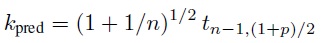
in place of z(1+p)/2. The factor kpred decreases to z(1+p)/2 as n → ∞ (Exercise 2.5). Therefore, when n is large, the interval within the limits of agreement can be interpreted as an approximate 100p% prediction interval for D. But this interval overestimates the extent of agreement because it is completely contained within the corresponding exact interval. This is an issue unless n is quite large. Besides, since the exact interval is not much harder to compute than the approximate one, the exact approach is preferred if a prediction interval is indeed desired. However, we have already argued in Section 2.6 that a prediction interval for D has limited usefulness in agreement evaluation because it only guarantees to cover the difference of a single future pair of measurements from the two methods. A tolerance interval for D is generally more suitable for this task. Of the two tolerance intervals discussed in Section 2.5—the ordinary interval (2.14) covering 100p% of the population and the interval from Exercise 2.7 covering the middle 100p% of the population—the latter appears more consistent with the Bland-Altman criterion.
2.8 TOTAL DEVIATION INDEX AND COVERAGE PROBABILITY
2.8.1 The Approaches
The measures total deviation index (TDI) and coverage probability (CP) provide two equivalent approaches for agreement evaluation using the Lin’s probability criterion presented in Section 2.6. Both are based on the statistical properties of the difference D. However, unlike the limits of agreement, they do not require the normality assumption for D (see, e.g., Chapter 10), although such an assumption is often made in practice.
For a specified large proportion p, the TDI measure is defined as:
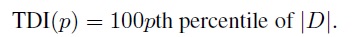 (2.23)
It is a non-negative measure, and a small value implies high agreement between the methods and the converse is true for a large value. When TDI(p) = 0 for all p, the methods have perfect agreement. By definition, the interval (−TDI(p), TDI(p)) represents a population range centered at zero that contains 100p% of the distribution of D.
For a specified small positive margin δ, the CP measure is defined as:
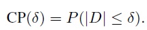 (2.24)
It represents the proportion of the population of D contained within the margin ± δ. It lies between zero and one, and a large value indicates high agreement. When CP(δ) = 1 for all δ, the methods have perfect agreement.
For specified (δ, p), Lin’s criterion (2.19) for sufficient agreement can be expressed in terms of the CP measure as CP(δ) > p. It can also be equivalently expressed in terms of the TDI measure as TDI(p) < δ because (Exercise 2.10)
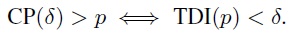 (2.25)
This equivalence implies that agreement can be evaluated using either of the two measures. In particular, with Lin’s criterion in the alternative, the agreement hypotheses (1.13) can be formulated in terms of either TDI or CP. Further, since the resulting alternative hypotheses are one-sided, they can be tested using appropriate one-sided confidence bounds (Section 1.11.2). The hypotheses (1.13) can be expressed in terms of TDI as
 (2.26)
These can be tested by computing an upper 100(1 − α)% confidence bound U for TDI(p) and comparing it with δ. Sufficient agreement is inferred if U < δ. Similarly, the hypotheses (1.13) can be expressed in terms of CP as
 (2.27)
These can be tested by computing a lower 100(1 − α)% confidence bound L for CP(δ) and comparing it with p. Sufficient agreement is inferred if L > p.
There is an interesting connection between performing the test based on TDI and employing a tolerance interval to evaluate agreement. It can be seen that if U is a 100(1 − α)% upper confidence bound for TDI(p), the interval (−U, U) is a tolerance interval containing 100p% of the distribution of D with 100(1 − α)% confidence (Exercise 2.11). By design, this tolerance interval is centered at zero. From Section 2.6, the decision rule based on a tolerance interval infers sufficient agreement if (−U, U) ⊂ (−δ, δ). Obviously, this rule is equivalent to inferring sufficient agreement on the basis of the test of hypotheses in (2.26). Thus, there is a one-to-one correspondence between a test of hypothesis and a tolerance interval for evaluating agreement using the Lin’s probability criterion.
Although the TDI and CP measures provide equivalent approaches for agreement evaluation, the TDI has one practical advantage. This has to do with the fact that the practitioners generally find it easier to specify p, which is commonly chosen to be one of {0.80, 0.90, 0.95}, than δ, whose value depends on the application. Of course, advance specification of both δ and p is necessary to formally test the agreement hypotheses. However, only p is needed in advance to compute the upper bound U for TDI(p). The practitioner can then evaluate agreement by examining whether the tolerance interval (−U, U) contains any unacceptably large differences, without having to explicitly provide a δ. On the other hand, advance specification of δ is necessary to perform inference using the CP measure. Because of this practical advantage, we only use TDI (with p = 0.90) in this book.
2.8.2 Normally Distributed Differences
If D ∼ N1 (ξ, τ2), the TDI defined by (2.23) can be obtained as the solution of the equation (Exercise 2.12)
 (2.28)
Alternatively, since

and D2/τ2 follows a noncentral χ2 distribution with 1 degree of freedom and noncentrality parameter ξ2/τ2, TDI(p) can be explicitly expressed as (Exercise 2.12)
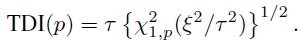 (2.29)
Generally it is easier to compute TDI using (2.29) than (2.28) because major statistical software packages have built-in functions for computing noncentral χ2 percentiles.
If D ∼ N1 (ξ, τ2), the CP defined by (2.24) can be determined as
 (2.30)
Following the approach that led to (2.29), CP(δ) can also be determined as a noncentral χ2 probability (Exercise 2.13).
2.9 INFERENCE ON AGREEMENT MEASURES
In this chapter, we have generally refrained from discussing point and interval estimation of agreement measures. The data may come from a variety of designs, for example, a paired design or a repeated measurements design. Once we have settled on a model for the data, the measures can be written as functions of the model parameters and can be estimated by simply plugging in the corresponding estimates. The standard errors of the estimates and the confidence intervals or bounds for the measures can be approximated using large-sample theory. When the sample size is not large enough for the standard approximations to be accurate, one can resort to bootstrap. These ideas are discussed in detail in the next chapter.
The measures like MSD, CCC, TDI, and CP are scalar functions of parameters. An exception is the limits of agreement approach in which two population percentiles are used to define the measure of agreement. Among the scalar measures, only CCC and TDI are used in this book. We also use the 95% of limits of agreement as a summary of the data, but do not use them for inference for the reasons explained in Section 2.7.
As argued in Section 1.11, we use confidence bounds instead of hypothesis tests for evaluating measures of agreement. Our emphasis is on lower bound for CCC and upper bound for TDI. However, we do use hypothesis tests for model comparison.
2.10 CHAPTER SUMMARY
- Different agreement measures quantify the extent of agreement differently, but all are functions of parameters of the bivariate distribution of (Y1, Y2).
- CCC is defined in terms of first-and second-order moments of (Y1, Y2). Its large positive values (nearing 1) imply high agreement.
- The measures MSD, TDI, and CP are based on the difference D. For MSD and TDI, small values (nearing zero) imply high agreement, whereas the converse is true for CP.
- For measures whose large values imply good agreement, for example, CCC and CP, a lower confidence bound can be used for evaluating agreement.
- For measures whose small values imply good agreement, for example, MSD and TDI, an upper confidence bound can be used for assessing the extent of agreement.
- TDI and CP provide equivalent metrics for agreement evaluation.
- Using an upper confidence bound for TDI is equivalent to using a tolerance interval for inference purposes.
- The limits of agreement are also based on the difference D. They are useful as an estimated summary measure of the data, but they should not be directly compared with the acceptable margin to infer sufficient agreement.
2.11 BIBLIOGRAPHIC NOTE
This chapter focuses only on common approaches for measuring agreement. Review of the literature on these and additional approaches can be found in Barnhart et al. (2007a) and Choudhary (2009). The MSD measure has been used by Hutson et al. (1998) and Choudhary and Nagaraja (2005b, c) for comparing extent of agreement in pairs of methods. The scaled versions of MSD, including CCC, have been considered by Lin (1989, 2000), Lin et al. (2002, 2007), Barnhart et al. (2007b), and Haber and Barnhart (2008).
The CCC was proposed by Lin (1989). However, the same measure, although not by the same name, appeared much earlier in Krippendorff (1970) in the psychology literature. The Krippendorff article, together with those of Fay (2005) and Haber and Barnhart (2006), discusses the issue of chance correction in the measure. Its connection and equivalence with intraclass correlation (McGraw and Wong, 1996) has been discussed in Lin (1989), Nickerson (1997), and Carrasco and Jover (2003). Undue influence of between-subject variation on the CCC and similar correlation-type measures has been pointed out by a number of authors, including Bland and Altman (1990), Müller and Büttner (1994), Atkinson and Nevill (1997), and Barnhart et al. (2007c). Lin and Chinchilli (1997) suggest comparing measurement ranges of datasets before comparing CCC estimates based on them. King and Chinchilli (2001a, b) present the generalized CCC, given by (2.8), in which MSD is replaced by E {g(Y1, Y2)}, where g is a distance function. Robust versions of CCC can be obtained by choosing appropriate g functions. King and Chinchilli (2001a) unify the treatment of chance-corrected agreement measures for continuous as well as categorical data by showing that, for some particular g functions, CCC reduces to kappa statistics (Cohen, 1960, 1968), which are popular measures of agreement for categorical data (see Chapter 12 for an introduction). The CCC has been generalized to deal with a variety of data types, summary of which can be found in Barnhart et al. (2007a) and Lin et al. (2011).
While the CCC has received the most attention in the statistical literature, the limits of agreement approach is the most popular approach in biomedical literature. It is proposed by Bland and Altman (1986). This article also recommends examining two-sided confidence intervals for the population percentiles that these limits estimate, and provides expressions for them. To evaluate agreement using the Bland-Altman criterion, Lin et al. (1998) formulate the problem as a test of agreement hypotheses (1.13) and provide an approximate test. This test employs two approximate one-sided confidence bounds, an upper bound for the upper percentile and a lower bound for the lower percentile. Liu and Chow (1997) provide an exact test for the same hypotheses (see Exercise 2.9), although the test was developed in a different context than ours. Instead of the limits of agreement, Carstensen et al. (2008) use a prediction interval for D and Ludbrook (2010) uses a tolerance interval for D. Ludbrook also recognizes that for agreement evaluation a tolerance interval is more appropriate than a prediction interval. Bland and Altman (1999) describe a nonparametric analog of the limits of agreement for the scenario when the normality assumption for D cannot be justified.
The TDI measure was proposed by Lin (2000). This article argues that directly testing (2.26) based on the TDI is difficult. Therefore, the TDI is approximated by a multiple of MSD, and a large-sample test is proposed. The CP measure was introduced by Lin et al. (2002). They provide a large-sample test for the hypothesis (2.27) based on CP. Wang and Hwang (2001) also present a test of (2.27), although in a different context. All these tests assume a random sample of differences. Choudhary and Nagaraja (2007) evaluate properties of these tests, and provide alternatives, including an exact test, that generally work better. This article also discusses the equivalence of the TDI and CP approaches and the connection between testing (2.26) and using a tolerance interval. Escaramis et al. (2010) provide another approach for inference on the TDI measure.
Guttman (1988) and Vardeman (1992) provide good introductions to prediction and tolerance intervals. See Krishnamoorthy and Mathew (2009) and Meeker et al. (2017) for book-length treatments. The former book also describes the tolerance factor approximation (2.15). The tolerance package of Young (2010) for the statistical software R provides additional methods for computing tolerance intervals.
EXERCISES
1. a. Verify the expression for CCC given in (2.6).
- Show that the second term on the right-hand side in (2.7) lies between zero and one, and the latter value corresponds to {ξ = 0, σ1 = σ2}.
- Verify the properties of CCC listed on page 55.
2. Consider two bivariate distributions for (Y1, Y2), both with ![]() and ρ = −0.1. The first distribution has (µ1, µ2) = (0, 0), and the second distribution has (µ1, µ2) = (−2, 2).
and ρ = −0.1. The first distribution has (µ1, µ2) = (0, 0), and the second distribution has (µ1, µ2) = (−2, 2).
- Which distribution exhibits worse agreement between Y1 and Y2 ? Why?
- Calculate CCC for both distributions. Which CCC is higher?
- Do you see any contradiction in the results in (a) and (b)? If yes, what explains the contradiction?
(This example is from Fay (2005).)
3. Suppose, based on paired measurements data, the CCC is estimated by replacing the population moments in its definition by their sample counterparts from (1.16). Consider two datasets presented in Table 2.1. Dataset A presents paired test-retest measurements of predicted maximal oxygen consumption (ml/kg/min) in 30 subjects using the Fitech test. Dataset B shows the same data as A but manipulated to get a less heterogeneous sample.
Table 2.1 Oxygen consumption (ml/kg/min) data for Exercise 2.3.
| Dataset A | Dataset B | |||
| Subject | Test | Retest | Test | Retest |
| 1 | 31 | 27 | 41 | 37 |
| 2 | 33 | 35 | 43 | 45 |
| 3 | 42 | 47 | 42 | 47 |
| 4 | 40 | 44 | 40 | 44 |
| 5 | 63 | 63 | 43 | 43 |
| 6 | 28 | 31 | 48 | 51 |
| 7 | 43 | 54 | 43 | 54 |
| 8 | 44 | 54 | 44 | 54 |
| 9 | 68 | 68 | 48 | 48 |
| 10 | 47 | 58 | 47 | 58 |
| 11 | 47 | 48 | 47 | 48 |
| 12 | 40 | 43 | 40 | 43 |
| 13 | 43 | 45 | 43 | 45 |
| 14 | 47 | 52 | 47 | 52 |
| 15 | 58 | 48 | 58 | 48 |
| 16 | 61 | 61 | 41 | 41 |
| 17 | 45 | 52 | 45 | 52 |
| 18 | 43 | 44 | 43 | 44 |
| 19 | 58 | 48 | 58 | 48 |
| 20 | 40 | 44 | 40 | 44 |
| 21 | 48 | 47 | 48 | 47 |
| 22 | 42 | 52 | 42 | 52 |
| 23 | 61 | 45 | 61 | 45 |
| 24 | 48 | 43 | 48 | 43 |
| 25 | 43 | 52 | 43 | 52 |
| 26 | 50 | 52 | 50 | 52 |
| 27 | 39 | 40 | 39 | 40 |
| 28 | 52 | 58 | 52 | 58 |
| 29 | 42 | 45 | 42 | 45 |
| 30 | 77 | 67 | 57 | 47 |
Reprinted from Atkinson and Nevill (1997), © 1997 Wiley, with permission from Wiley.
- Verify that both datasets have exactly the same differences in test-retest measurements and Dataset A has larger between-subject variation than B.
- Estimate the correlation ρ from both data. Which estimate is higher? Why?
- Estimate the second factor on the right side in (2.7) from both data. How do the estimates compare?
- Estimate CCC for both data. Which estimate is higher?
- What do you conclude about the dependence of CCC on between-subject variation?
(This example is from Atkinson and Nevill (1997).)
4. Verify the relation (2.12) between the probability of covering one future observation and the expected probability content of a prediction interval.
5. Consider a 100p% prediction interval of the form (2.13) for a single observation from a normal distribution using a random sample from this distribution.
- Verify the expression (2.17) for expected probability content of the interval.
- Show that the interval in (2.18) is a 100p% prediction interval.
- Show that the factor kpred in (2.18) is greater than z(1+p)/2 and decreases to z(1+p)/2 as n → ∞.
6. Perform a Monte Carlo simulation study to evaluate the accuracy of the approximation (2.15) for the tolerance factor ktol. You can examine how close the probability on the left in the definition (2.10) is to the nominal confidence level as a function of p, α, and n.
7. Consider a tolerance interval of the form (2.13) using a random sample from a normal distribution that contains the middle 100p% of the population.
Show that this interval is
 ± kmid S, where kmid = kmid(n, p, α) solves for k the equation
Obtain an expression for the probability on the left.
- Show that kmid > ktol, where ktol is the tolerance factor for the usual interval (2.14). This implies that the new interval is wider than the usual interval. Does this seem intuitively reasonable? Explain.
8. Compute tolerance and prediction intervals with (p, 1 − α) = (0.90, 0.95) for the difference in test-retest measurements of Exercise 2.3, and interpret them. Assume normality for the differences. Can you justify this assumption?
9. The evaluation of agreement using Bland-Altman criterion can be performed by testing the following hypotheses which are of the general form (1.13):
 (2.31)
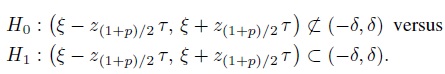
This exercise derives an intersection-union test (Casella and Berger, 2001, Chapter 8) of these hypotheses assuming we have a random sample D1,...,Dn from the population of D ∼ N1 (ξ, τ2). This test was proposed by Liu and Chow (1997) in a context different from agreement evaluation.
Argue that the hypotheses in (2.31) can be divided into two subhypotheses involving the lower and the upper percentiles,

and

respectively, so that H0 is a union of H01 and H02, and H1 is an intersection of H11 and H12. The intersection-union test rejects H0 when both H01 and H02 are rejected. Show that if a level α test is used for each subhypothesis, then the level of the intersection-union test is also α.
- Show that rejecting H01 in favor of H11 if
 provides a level α test, where
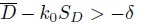
- Similarly, show that rejecting H02 in favor of H12 if
 provides a level α test.
 Deduce that rejecting H0 in favor of H1 if
provides the desired intersection-union test with level α.
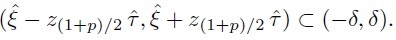
- Can the interval
 be interpreted as a tolerance interval? Explain.
10. For specified (δ, p), establish the equivalence (2.25) of TDI and CP criteria for sufficient agreement.
11. Show that if U is a 100(1 − α)% upper confidence bound for TDI(p), the interval (−U, U) is a tolerance interval containing 100p% of the distribution of D with 100(1 − α)% confidence.
12. Show that if D ∼ N1 (ξ, τ2), TDI(p) can be obtained by solving
with respect to t for t > 0. Further, verify the expression (2.29) for TDI(p).
13. Show that if D ∼N1 (ξ, τ2), CP(δ) can be written as (2.30). Also express CP(δ) as a noncentral χ2 probability.