CHAPTER 7
DATA FROM MULTIPLE METHODS
7.1 PREVIEW
So far we have focussed on method comparison studies involving two measurement methods. Quite often, more than two methods are compared in the same study. It is of interest here to perform multiple comparisons of method pairs to evaluate the extent of similarity and agreement. This chapter generalizes the data models in Chapters 4 and 5 to accommodate multiple methods where we assume these methods are fixed rather than randomly chosen ones. It considers simultaneous inference on pairwise measures of similarity and agreement that adjusts for multiplicity. The measurements may or may not be repeated and the design may not be balanced. But it is assumed that the data are homoscedastic and the measurement methods have the same scale. Two case studies are used for illustration.
7.2 INTRODUCTION
Suppose there are J ( ≥ 2) measurement methods under comparison. Here J is considered fixed and known. Two data designs are of interest. One is where the data are unreplicated , that is, there is only one measurement from each method on every subject. These data consist of Yij , j = 1 ,..., J , i = 1,...,n , with Yij representing the measurement from the jth method on the ith subject. There are a total of N = Jn observations and they form an extension of the paired measurements data considered in Chapter 4.
The other design is where the measurements are repeated. These data are denoted as Yijk, k = 1,...,mij, j = 1 ...,J , i = 1 ,...,n, with Yijk as the kth measurement of the jth method on the ith subject. This setup generalizes the one considered in Chapter 5. When mi1 = ... = mij, the common value is denoted by mi. Also, ![]() mij is the number of observations on subject i, and
mij is the number of observations on subject i, and ![]() is the total number of observations in the data. As before, the repeated measurements may be unlinked or linked. In the linked case, mij = mi for all j = 1,..., J by design, and Mi = Jmi. As before, the steps in the analysis of data include displaying them, modeling them, and evaluation of similarity and agreement. First we explain how the last step calls for multiple comparisons as done in analysis of variance (ANOVA) models. Methods play the role of treatments in those models.
is the total number of observations in the data. As before, the repeated measurements may be unlinked or linked. In the linked case, mij = mi for all j = 1,..., J by design, and Mi = Jmi. As before, the steps in the analysis of data include displaying them, modeling them, and evaluation of similarity and agreement. First we explain how the last step calls for multiple comparisons as done in analysis of variance (ANOVA) models. Methods play the role of treatments in those models.
To understand the parallel between method comparison studies with multiple methods and ANOVA, it is helpful to recall that the ANOVA is concerned with comparison of more than two treatments, primarily through their means. The multiplicity of comparisons gives rise to the problem of multiple comparisons , which warrants simultaneous inference on the contrasts of interest in the treatment means. A contrast in the means is a linear combination of the means with the property that the coefficients add up to zero. A difference in two means is the simplest example of a contrast. More generally, if there are J treatments, then the ![]() pairwise differences of treatment means may be the contrasts of interest. Alternatively, if one treatment serves as the control, then the differences in the means of the remaining J −1 treatments with the control mean may be the contrasts of interest. There are others that may also be of interest, for example, difference between the mean of a treatment and the average of all the treatments. For simultaneous inference on the contrasts, one can employ an appropriate set of simultaneous 100(1 − α)% confidence intervals, guaranteeing that all the intervals simultaneously cover their respective contrasts with at least 1 − α probability. Because the simultaneous intervals adjust for the multiplicity of inferences, they are more relevant than the separate individual confidence intervals. If this adjustment is not made, the simultaneous coverage probability of the individual 100(1 − α)% confidence intervals may be much less than 1 − α (Exercise 7.1).
pairwise differences of treatment means may be the contrasts of interest. Alternatively, if one treatment serves as the control, then the differences in the means of the remaining J −1 treatments with the control mean may be the contrasts of interest. There are others that may also be of interest, for example, difference between the mean of a treatment and the average of all the treatments. For simultaneous inference on the contrasts, one can employ an appropriate set of simultaneous 100(1 − α)% confidence intervals, guaranteeing that all the intervals simultaneously cover their respective contrasts with at least 1 − α probability. Because the simultaneous intervals adjust for the multiplicity of inferences, they are more relevant than the separate individual confidence intervals. If this adjustment is not made, the simultaneous coverage probability of the individual 100(1 − α)% confidence intervals may be much less than 1 − α (Exercise 7.1).
In a method comparison study with two methods, there is only one method pair of interest. But if more than two methods are involved, there will be several such pairs. For example, if there is a reference method in the comparison, we may be interested in comparing each of the other methods with the reference method. This results in a total of J − 1 method pairs. On the other hand, if the study does not have a reference method, we may be interested in comparing each method with every other method, resulting in a total of ![]() distinct method pairs. Thus, any inference we do for one method pair, viz., evaluation of agreement, has to be done multiple times. The comparisons with a reference and all-pairwise comparisons are akin to comparisons with a control and all-pairwise comparisons in an ANOVA setting. There is, however, one crucial difference. In ANOVA, the treatments are compared primarily through the contrasts in their means. But in method comparison studies, the measurement methods are compared through pairwise measures of similarity and agreement. In addition to the contrasts in the means, they also involve variances and covariances.
distinct method pairs. Thus, any inference we do for one method pair, viz., evaluation of agreement, has to be done multiple times. The comparisons with a reference and all-pairwise comparisons are akin to comparisons with a control and all-pairwise comparisons in an ANOVA setting. There is, however, one crucial difference. In ANOVA, the treatments are compared primarily through the contrasts in their means. But in method comparison studies, the measurement methods are compared through pairwise measures of similarity and agreement. In addition to the contrasts in the means, they also involve variances and covariances.
Despite the difference in the target parametric functions, the ANOVA analogy makes it clear that to evaluate similarity and agreement of the method pairs of interest, we need appropriate simultaneous confidence intervals, one-sided or two-sided, for the pairwise measures of similarity and agreement. The simultaneous intervals can, of course, be obtained by applying a Bonferroni adjustment to the individual intervals. It amounts to using 100(1 − α/Q)% , with Q denoting the number of comparisons of interest, as the level of confidence for each individual interval (Exercise 7.1). But such an adjustment is known to be conservative in that the simultaneous coverage probability of the Q intervals may be much greater than the nominal level of 100(1 − α)%. Further, the intervals may become too wide to be helpful for our purpose.
7.3 DISPLAYING DATA
The graphical tools for displaying data from two methods are easily adapted for multiple methods. For example, the trellis plot retains the same basic appearance as before except that each row now shows a subject’s measurements from all methods, with different symbols, rather than two methods. The plot, however, may look cluttered if there are several methods and they have small within-subject variation, making it difficult to distinguish between the methods. Although the cluttering itself may be informative in that it may suggest similar characteristics for the methods, one may supplement the trellis plot with side-by-side boxplots of data from different methods to get a clearer comparison of their marginal distributions.
Besides the trellis plot, the scatterplot and the Bland-Altman plot are also used to display data from two methods. When there are more than two methods, we can make a “matrix” of the pairwise plots. In its standard form, a matrix of plots is an arrangement of scatterplots on a square grid, consisting of one plot for each pair of distinct variables. The panels in the diagonal either are left empty or contain the labels of the methods. Moreover, the same pairs of variables are plotted in the panels above and below the diagonal, but with variables on horizontal and vertical axes interchanged.
For method comparison data, we can devise a variation of the standard matrix to simultaneously display both scatterplots and Bland-Altman plots. To describe it, suppose each subject in the study is measured once using J methods, Y1,...,YJ. The matrix consists of a J × J grid of boxes. The J boxes on the diagonal only contain the method labels from 1 to J. The J(J − 1)/2 boxes below and above the diagonal, respectively, contain the scatterplots and the Bland-Altman plots. The box in row i and column j below the diagonal (i.e., i > j ) contains the scatterplot of (Yj, Yi). The box in row i and column j above the diagonal (i.e., i < j) contains the corresponding Bland-Altman plot—the scatterplot of ((Yi + Yj) /2, Yj − Yi). Of course, the positions of the scatterplots and the Bland-Altman plots can be interchanged. One can further embellish the matrix by displaying either histograms or boxplots of the variables on the diagonal. The preceding construction assumes unreplicated data. If the measurements are repeated, then as in Chapter 5, one can either use a randomly chosen measurement from a subject or the average of its multiple measurements.
7.4 EXAMPLE DATASETS
We now introduce two datasets with displays. Their detailed analysis is presented in Section 7.10.
7.4.1 Systolic Blood Pressure Data
These data were collected in a study to compare systolic and diastolic blood pressure measurements (in mm Hg) taken by three observers using a mercury sphygmomanometer and one observer using a digital sphygmomanometer. The digital one is cheaper and is easier to use than its mercury counterpart. The four observers in the comparison are as referred to as MS1, MS2, MS3, and DS, respectively. They are labeled as methods 1, 2, 3, and 4, respectively. It is of interest to compare the three MS observers among themselves and also with the DS observer, essentially implying all-pairwise comparisons. The measurements in this study are not replicated; each observer takes only one measurement on each subject. There are 228 subjects in the study. Here we focus only on the systolic measurements. They range from 82 to 236 mm Hg.
Figure 7.1 shows a trellis plot of the data. Each row in the plot has four observations, one per observer. The plot has a cluttered look, but the large overlap in the symbols implies that the measurements from the four observers tend to be close. It is also apparent that DS often has the largest measurement. The within-subject variation of the observations is small relative to the between-subject variation. There is no evidence of heteroscedasticity as the within-subject spread remains largely similar throughout the measurement range. The boxplots presented in Figure 7.2 show small differences in the marginal distributions of the observers. These distributions appear right-skewed.
Figure 7.3 displays a matrix of scatterplots and Bland-Altman plots for systolic blood pressure data. The scatterplots show high pairwise correlations among the four observers. The Bland-Altman plots do not exhibit any trend, implying a common scale for the observers, or nonconstant vertical scatter, confirming homoscedasticity of the data. The centers of the plots suggest small differences in the observers’ means.
7.4.2 Tumor Size Data
These data consist of tumor sizes (in cm) of 40 lesions measured by five readers. The tumor sizes are “unidimensional” in that they are based on the longest diameter of the lesion. Each measurement is replicated twice. The replications are assumed to be unlinked. The measurements range from 1 to 9 cm.
Figure 7.4 presents a trellis plot of the data. Each row in this plot has ten observations, two per reader. The plot is not as cluttered as the plot of the previous dataset. The within-subject variation here is relatively large compared to what we have seen for other datasets presented in this book. But it does not seem to change with the magnitude of measurement. It is also evident that reader 2 is somewhat deviant compared to the rest as her/his measurements tend to be the smallest. Reader 3 often has the largest measurements. The boxplots presented in Figure 7.5 clarify these differences in the readers’ marginal distributions. Both replications of measurements have been used in this plot. Alternatively, one can average the two replications or randomly select one of the replications without any qualitative change in the conclusions. The trellis plot shows considerable subject × reader interaction. It is confirmed by crossing of the line segments for different subjects in the interaction plot in Figure 7.6.
Figure 7.7 presents a matrix of scatterplots and Bland-Altman plots for tumor size data. The scatterplots show moderately high p correlations among the five readers.
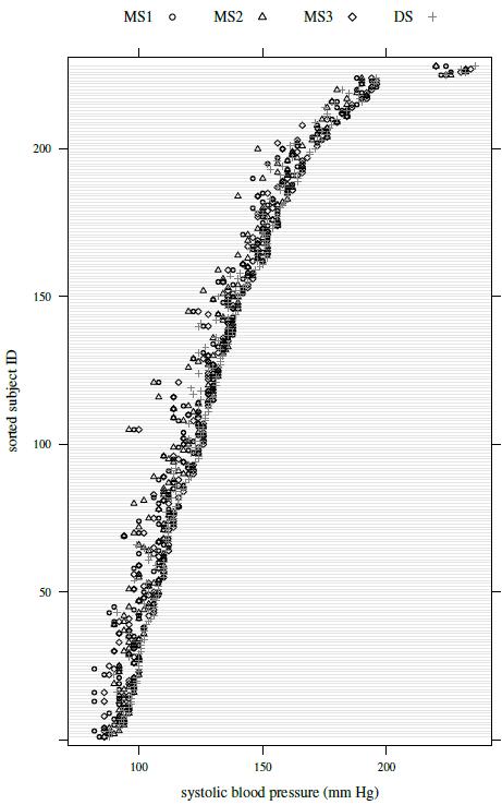
Figure 7.1 Trellis plot of systolic blood pressure data. The symbols for the four observers are given at the top of the plot.
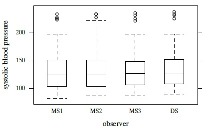
Figure 7.2 Side-by-side boxplots for systolic blood pressure data.
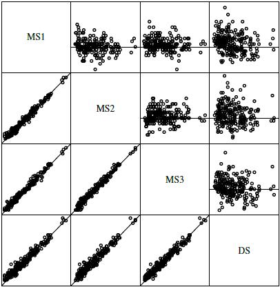
Figure 7.3 A matrix of scatterplots with line of equality (below the diagonal) and Bland-Altman plots with zero line (above the diagonal) for systolic blood pressure data. The measurements range from 82 to 236 mm Hg and their differences range from −16 to 30 mm Hg.
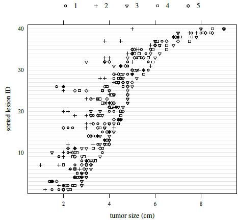
Figure 7.4 Trellis plot of tumor size data. The symbols for the five readers are given at the top of the plot.
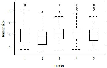
Figure 7.5 Side-by-side boxplots for tumor size data.
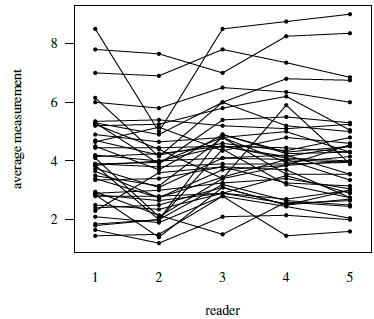
Figure 7.6 Interaction plot for tumor size data depicting lesion × reader interaction.
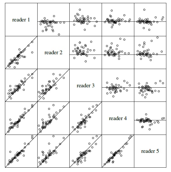
Figure 7.7 A matrix of scatterplots with line of equality (below the diagonal) and Bland-Alt man plots with zero line (above the diagonal) for tumor size data. One measurement from each reader on every subject is randomly selected for this plot. The measurements range from 1 to 9 cm and their differences range from –3 to 4 cm.
The Bland-Altman plots show that the readers, though on the same scale, have somewhat different means. The data appear homoscedastic.
7.5 MODELING UNREPLICATED DATA
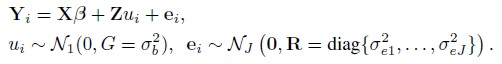
Assuming that all the J ( ≥ 2) methods have a common scale, the data Yij, j = 1,...,J, i = 1,...,n can be modeled by the following straightforward extension of the mixed-effects model (4.1) for paired measurements data:
Here βj is the difference in the fixed biases of methods j and 1. The intercept β0 in (4.1) is now denoted as β2. As in (4.1), the true values bi follow independent ![]() ) distributions, the random errors eij follow independent
) distributions, the random errors eij follow independent ![]() distributions, and the bi and eij are mutually independent. For notational convenience, we define β1 = 0 as a known constant, allowing us to write the model as
distributions, and the bi and eij are mutually independent. For notational convenience, we define β1 = 0 as a known constant, allowing us to write the model as
This model allows each method to have its own error variance. The J measurements (Yi1,...,YiJ) on subject i share the same true value bi. Consequently, we see that (Exercise 7.2) these measurements are i.i.d. as (Y1,...,YJ), where
 (7.2)
(7.2)Thus, the means and variances of the measurements are
and
is the common covariance between measurements from any two methods on the same subject. The dependence in the measurements is induced by the sharing of the common true value bi. This model has a total of 2J + 1 unknown parameters,
When J = 2, the model (7.1) and the associated population distribution (7.2) reduce to their respective counterparts for paired measurements data in (4.1) and (4.2). Let Djl = Yl − Yj be the difference in measurements of the method pair (j, l), j ≠ l. It follows from (7.2) that
Moreover, the differences associated with different method pairs are independent.
7.6 MODELING REPEATED MEASUREMENTS DATA
As in Chapter 5, the modeling of repeated measurements data depends on whether the measurements are unlinked or linked. We consider these cases in turn, assuming as before that the methods have the same scale and J > 2. The models reduce to their counterparts with J = 2 provided an additional equal variance assumption is made.
7.6.1 Unlinked Data
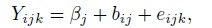
To model the unlinked data Yijk, k = 1,... mij, j = 1,..., J (> 2), i = 1,..., n, we can extend the mixed-effects model (5.1) as
where, as in (7.1), β1 = 0 , and for j > 2, βj represents the difference in the fixed biases of methods j and 1. Moreover, the intercept β0 in (5.1) has been relabeled as β2. As in (5.1), it is assumed that the true values bi follow independent ![]() distributions; the interactions bij follow independent
distributions; the interactions bij follow independent ![]() distributions; the random errors eijk follow independent
distributions; the random errors eijk follow independent ![]() distributions; and bi, bij, and eijk are mutually independent.
distributions; and bi, bij, and eijk are mutually independent.
The model (7.4) for J > 2 allows the variance of the interaction effect to depend on the method, whereas in the model (5.1) for J = 2, the variance is assumed constant across the two methods. Thus, (7.4) reduces to (5.1) for J = 2 provided ![]() . When k = 1, that is, the measurements are not replicated, the effect of the interaction term bij in (7.4) gets confounded with that of the error term and has to be removed from the model. Doing so yields the model (7.1) in Section 7.5 as a special case of (7.4).
. When k = 1, that is, the measurements are not replicated, the effect of the interaction term bij in (7.4) gets confounded with that of the error term and has to be removed from the model. Doing so yields the model (7.1) in Section 7.5 as a special case of (7.4).
Proceeding as in Section 5.4.1, we can average over the J + 1 mutually independent random effects bi, bi1,...,biJ in (7.4) to see that the vector of Mi measurements on subject i follows an independent Mi-variate normal distribution with means and variances (Exercise 7.3)
The covariance between measurements depends on whether or not they come from the same method. Any two measurements of method j have the covariance
whereas any two measurements from different methods have the common covariance
The subscripts k and p here may be equal or different. The model (7.4) has a total of 3J + 1 unknown parameters,
Our next task is to obtain the distribution of (Y1,...,YJ) induced by the model (7.4). Recall that this vector contains one measurement from each of the J methods on a randomly selected subject from the population. For this we proceed in the usual manner to drop the subscripts i and k in (7.4), getting its companion model as
Here b , bj , and ej are identically distributed as bi , bij , and eijk , respectively. Upon averaging over the distribution of (b , b1 ,...,bJ) , we get (Exercise 7.4)
 (7.9)
(7.9)For the difference Djl = Yl − Yj, j ≠ l , it follows that
The distribution in (7.9) is used to derive measures of similarity and agreement. The repeated measurements also allow evaluation of repeatability of each method. Following Section 5.6, to derive measures of repeatability, we need the distributions of the pairs ![]() where
where ![]() is a replication of ( Y1 ,...,YJ) on the same subject. The companion model for
is a replication of ( Y1 ,...,YJ) on the same subject. The companion model for ![]() induced by the data model (7.4) is
induced by the data model (7.4) is
where ![]() is an independent copy of (e1, ...,eJ) in (7.8). It follows from (7.8) and (7.11) that (Exercise 7.4)
is an independent copy of (e1, ...,eJ) in (7.8). It follows from (7.8) and (7.11) that (Exercise 7.4)
 (7.12)
For the difference Dj = Yj − ![]() in two replications of method J, from (7.12), we have
in two replications of method J, from (7.12), we have
7.6.2 Linked Data
As in Section 5.4.2, the model for the measurements (Yi1k,...,YiJk) linked by the common time k = 1,...,mi for subjects i = 1,...,n is obtained by simply adding the random effect ![]() of time k to the model (7.4) for unlinked data. This yields
of time k to the model (7.4) for unlinked data. This yields
where the ![]() , also interpreted as subject × time interaction, follow independent
, also interpreted as subject × time interaction, follow independent ![]() distributions. They are mutually independent of the other random terms in the model that continue to follow the same distributions as in (7.4). This model reduces to the model (5.1) for J = 2 if a common variance
distributions. They are mutually independent of the other random terms in the model that continue to follow the same distributions as in (7.4). This model reduces to the model (5.1) for J = 2 if a common variance ![]() is assumed for the subject × method interactions.
is assumed for the subject × method interactions.
Averaging over the J + mi + 1 mutually independent random effects, namely,
we see that the vector of Mi = Jmi observations on subject i follows an independent Mi-variate normal distribution with (Exercise 7.5)
The covariance in any two measurements is induced by the common random effects they share. Therefore, the covariances depend on whether or not the measurements involved are taken by the same method and at the same time. For measurements taken by method j but at different times,
For measurements taken by different methods but at the same time,
For measurements taken by different methods at different times,
The model (7.14) has a total of 3J + 2 unknown parameters,
Compared to the model (7.4), the additional parameter here is subject × time interaction variance ![]() .
.
Next, we need the distribution of (Y1, ...,YJ) induced by the model (7.14) to derive measures of similarity and agreement. Proceeding along the lines of Section 5.4.2, it can be seen from Exercise 7.6 that this distribution is J -variate normal with mean vector
and covariance matrix
 (7.20)
This implies
As seen in Section 5.4.2 before, this distribution is identical to the one in (7.10) for unlinked data.
Analogous to Section 5.6.2, we also need the distributions of the pairs (Yj, Yj∗), j = 1 ,..., J to derive the measures of repeatability. Here ![]() is another set of measurements taken on the same subject that produces (Y1, ...,YJ). From Exercise 7.6, the desired distribution is
is another set of measurements taken on the same subject that produces (Y1, ...,YJ). From Exercise 7.6, the desired distribution is
 (7.22)
It follows that
7.7 MODEL FITTING AND EVALUATION
All the three models—(7.1), (7.4), and (7.14)—can be fit by the ML method using any software that can fit mixed-effects models (see Section 7.12). The software would provide ML estimates of model parameters, predicted values of random effects, fitted values, and raw as well as standardized residuals. These quantities can be used as in Section 3.2.4 to perform model evaluation. We have used β1 = 0 as a known parameter for notational convenience. Its “estimate” can be taken as ![]() .
.
Specifically, for the model (7.1) for unreplicated data, we get the ML estimates
the predicted true values ![]() , the fitted values
, the fitted values ![]() , the raw residuals
, the raw residuals ![]() , and the standardized residuals
, and the standardized residuals ![]() . Recall from Chapter 4 that the variance components in (4.1) for j = 2 are not estimated reliably with unreplicated data. No such difficulty arises when j > 2.
. Recall from Chapter 4 that the variance components in (4.1) for j = 2 are not estimated reliably with unreplicated data. No such difficulty arises when j > 2.
For the model (7.4) for unlinked repeated measurements data, we also have the ML estimates ![]() and predicted subject × method interactions
and predicted subject × method interactions ![]() ; and the fitted values are
; and the fitted values are ![]() . For the model (7.14) for linked repeated measurements data, we additionally have the ML estimate
. For the model (7.14) for linked repeated measurements data, we additionally have the ML estimate ![]() and predicted subject × time interactions
and predicted subject × time interactions ![]() ; and the fitted values are
; and the fitted values are ![]() . In both cases, the raw and the standardized residuals are
. In both cases, the raw and the standardized residuals are ![]() , respectively.
, respectively.
Sometimes the default models (7.4) and (7.14) fail to provide reliable estimates of all the variance components. One remedy may be to simplify the model by assuming equal variances ![]() for the subject × method interactions bij (see Exercise 7.11). Another may be to drop the bi term from the model, assume that (bi1,...,biJ) follow independent multivariate normal distributions with zero mean and an unstructured covariance matrix, and take β1 to be an unknown parameter (see Exercise 7.12). The models for both unreplicated and repeated measurements data also assume homoscedastic errors. If this assumption is in doubt, perhaps even after a log transformation of data, then the models can be extended as in Chapter 6 to allow heteroscedastic errors (see also Chapter 8). This chapter’s methodology of evaluation of similarity and agreement can be easily adapted to work under the new models.
for the subject × method interactions bij (see Exercise 7.11). Another may be to drop the bi term from the model, assume that (bi1,...,biJ) follow independent multivariate normal distributions with zero mean and an unstructured covariance matrix, and take β1 to be an unknown parameter (see Exercise 7.12). The models for both unreplicated and repeated measurements data also assume homoscedastic errors. If this assumption is in doubt, perhaps even after a log transformation of data, then the models can be extended as in Chapter 6 to allow heteroscedastic errors (see also Chapter 8). This chapter’s methodology of evaluation of similarity and agreement can be easily adapted to work under the new models.
7.8 EVALUATION OF SIMILARITY AND AGREEMENT
In Chapters 4 and 5, measures of similarity and agreement were derived from the bivariate normal distribution of (Y1, Y2) induced by the model assumed for the data. Two measures of similarity were considered. One is the intercept β0, representing the difference in fixed biases or the means of the two methods. This quantity is β2 − β1 in the notation of the present chapter (because β1 = 0, by definition). The other is the ratio of precisions of the two methods, ![]() . With repeated measurements, a modification of this precision ratio,
. With repeated measurements, a modification of this precision ratio, ![]() , is also considered to take the subject × method interactions into account. For measures of agreement, as usual we consider CCC and TDI.
, is also considered to take the subject × method interactions into account. For measures of agreement, as usual we consider CCC and TDI.
When J > 2, we have multiple method pairs of interest, say, Q. For example, Q = J −1 for comparisons with a reference, and ![]() for all-pairwise comparisons. Associated with each of the Q method pairs, there is one value for every measure of similarity and agreement—all derived from the J -variate normal distribution of (Y1, ...,YJ) induced by the assumed data model. The parameters of this distribution are given by (7.2) for unreplicated data, by (7.9) for unlinked repeated measurements data, and by (7.19) and (7.20) for linked repeated measurements data.
for all-pairwise comparisons. Associated with each of the Q method pairs, there is one value for every measure of similarity and agreement—all derived from the J -variate normal distribution of (Y1, ...,YJ) induced by the assumed data model. The parameters of this distribution are given by (7.2) for unreplicated data, by (7.9) for unlinked repeated measurements data, and by (7.19) and (7.20) for linked repeated measurements data.
If the method pair (j, l) is of interest for some j ≠ l ∈ {1, ..., J}, then the measures based on (Yj, Yl) can be obtained by essentially taking their counterparts based on (Y1, Y2) and replacing the subscripts (1, 2) with (j, l). This leads to βl − βj as the bias difference, ![]() as the precision ratio, and
as the precision ratio, and
as the modified precision ratio that takes the subject × method interactions into account. Note that when only two methods are involved, equal interaction variances are assumed in (7.24). From (4.11) and (7.2), the two agreement measures for unreplicated data can be expressed as (Exercise 7.7)
 (7.25)
Likewise, for unlinked repeated measurements data, from (5.19), (5.21), and (7.9) they can be expressed as
 (7.26)
For linked repeated measurements data, from (5.20), (7.19), and (7.20) the CCC is
 (7.27)
and the TDI is the same as in (7.26). This happens because the difference Djl has the same distribution for both unlinked and linked data—see (7.10) and (7.21). The expressions for these measures are verified in Exercise 7.7.
It is apparent from the ANOVA analogy in Section 7.2 that for similarity evaluation we need to examine two-sided simultaneous confidence intervals for the Q values of each similarity measure. Likewise, for agreement evaluation we need to examine one-sided simultaneous confidence bounds for the Q values of an agreement measure. These bounds, in addition to allowing us to infer which method pairs, if any, have sufficient agreement for interchangeable use, also allow us to compare the extent of agreement among the method pairs. As before, the ML estimators of the measures are obtained by replacing the unknown parameters in their expressions by their ML estimators, and the large-sample theory is used to get standard errors and simultaneous confidence bounds and intervals. The latter are of the same form as their individual counterparts,
possibly on a transformed scale that makes the parameter range to be the entire real line. The critical point is now a percentile of an appropriate function of a Q-variate normal vector with standard normal marginals (see Section 3.3.2). One may also proceed as in Section 3.3.6 to perform a test of homogeneity to test the null hypothesis of equality of the Q values of the measure.
The 95% limits of agreement for (Yj, Yl) can be computed using the distributions of Djl in (7.3), (7.10), and (7.21). These limits are
for unreplicated data, and are
for unlinked as well as linked repeated measurements data. Note that no multiplicity adjustment has been made in these limits.
7.9 EVALUATION OF REPEATABILITY
Section 5.6 discusses measures of repeatability that evaluate intra-method agreement when repeated measurements data are available. A measure of repeatability for method j is essentially a measure of agreement between ![]() —two repeated measurements of method j on the same subject. From the distributions of
—two repeated measurements of method j on the same subject. From the distributions of ![]() and the associated difference Dj in (7.12) and (7.13), the repeatability analogs of CCC and TDI for unlinked data can be found as (Exercise 7.8)
and the associated difference Dj in (7.12) and (7.13), the repeatability analogs of CCC and TDI for unlinked data can be found as (Exercise 7.8)
 (7.30)
For linked data, using (7.22) and (7.23) we obtain (Exercise 7.8)
 (7.31)
Recall from Section 5.6 that CCCj represents the intraclass correlation between Yj and Yj∗. For unlinked data, it additionally represents the reliability of method j in the sense of (1.4).
One-sided confidence bounds for the repeatability measures are obtained in exactly the same manner as the agreement measures with the exception that the individual bounds suffice here. Although one can use simultaneous bounds, they are not really needed because the repeatability measures are primarily concerned with establishing a benchmark for how much agreement is possible, and not examining whether the methods have sufficiently high repeatability. The latter does not require adjustment for multiplicity of inferences.
One can use the distributions of Dj in (7.13) and (7.23) to get 95% limits of intra-method agreement for method j =1 ,..., J for unlinked data as
and for linked data as
7.10 CASE STUDIES
7.10.1 Systolic Blood Pressure Data
The systolic blood pressure data introduced in Section 7.4 has measurements (in mm Hg) on n = 228 subjects taken by three observers—MS1, MS2, and MS3—using a mercury sphygmomanometer, and one observer—DS—using a digital sphygmomanometer. We call these observers methods 1, 2, 3, and 4, respectively. The measurements are not replicated. The interest is in comparing the MS observers among themselves and also with the DS observer. These are ![]() pairwise comparisons. An exploratory data analysis based on the trellis plot in Figure 7.1, boxplots in Figure 7.2, and a matrix of scatterplots and Bland-Altman plots in Figure 7.3 shows that the observers are highly correlated and have a common scale, but small differences exist in their means. The data appear homoscedastic.
pairwise comparisons. An exploratory data analysis based on the trellis plot in Figure 7.1, boxplots in Figure 7.2, and a matrix of scatterplots and Bland-Altman plots in Figure 7.3 shows that the observers are highly correlated and have a common scale, but small differences exist in their means. The data appear homoscedastic.
We fit the mixed-effects model (7.1) to the data. Figure 7.8 shows the resulting residual plot. It appears centered at zero and does not have any trend or nonconstant vertical scatter. Model diagnostics (not presented here) show that the normality assumption is adequate for the errors. But the random effects appear right-skewed, and this explains the right-skewness seen in the boxplots in Figure 7.2. We ignore this as usually a moderate departure from normality of random effects does not have much impact on the overall conclusions of a method comparison data analysis.
Table 7.1 summarizes ML estimates of the nine model parameters. Substituting the estimates in (7.2) gives the fitted multivariate normal distribution of (Y1, Y2, Y3, Y4), with means (128.69, 128.98, 130.18, 131.45), variances (938.30, 942.63, 937.21, 961.07), and common covariance 928.53. All pairwise correlations exceed 0.975. Both the mean and variance are largest for DS and smallest for MS1. It can also be seen that the pairwise differences among three MS observers have means between 0.3 and 1.2 and standard deviations between 4.3 and 4.9. Moreover, the differences between the MS observers and DS have means between 1.3 and 2.8 and standard deviations between 6.4 and 6.8. Neither the means nor the standard deviations are particularly large.
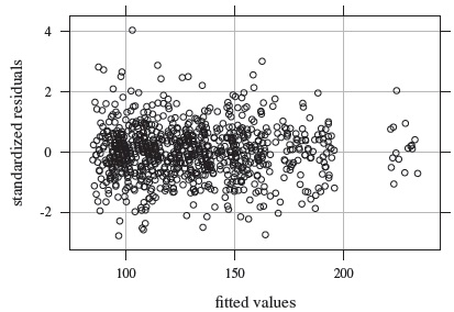
Figure 7.8 Residual plot for systolic blood pressure data.
Table 7.1 Summary of parameter estimates for systolic blood pressure data. Methods 1, 2, 3, and 4 refer to the observers MS1, MS2, MS3, and DS, respectively.
| Parameter | Estimate | SE | 95 % Interval |
| β2 | 0.29 | 0.32 | (−0.34, 0.92) |
| β3 | 1.49 | 0.28 | (0.93, 2.05) |
| β4 | 2.75 | 0.43 | (1.91, 3.60) |
| µb | 128.69 | 2.03 | (124.72, 132.67) |
| 6.83 | 0.09 | (6.65, 7.02) | |
| 2.28 | 0.14 | (2.00, 2.56) | |
| 2.65 | 0.12 | (2.41, 2.89) | |
| 2.16 | 0.15 | (1.86, 2.46) | |
| 3.48 | 0.10 | (3.28, 3.69) |
Table 7.2 presents estimates of similarity measures along with two-sided 95% simultaneous confidence intervals for the six pairwise bias differences and precision ratios. The critical point used in the intervals for the bias differences is 2.555, and it is 2.557 for the log of precision ratios. Although only one interval for bias difference contains zero and the rest lie to the right of zero, none of the interval endpoints is too far from zero. Thus, the biases and hence the means of the observers can be considered practically equal. The same, however, cannot be said for the precisions. The first three intervals for precision ratios contain 1 but the last three lie quite below 1. Thus, the MS observers can be considered equally precise, but DS is less precise than them. In fact, in the best case, DS may be about 70% as precise as an MS observer, but in the worst case, its precision may be less than 20% of an MS observer. Taken together, these findings suggest that the MS observers have similar characteristics among themselves, but DS differs from them by being less precise.
Table 7.2 Estimates and 95% simultaneous confidence intervals for all-pairwise bias differences and precision ratios for systolic blood pressure data. Methods 1, 2, 3, and 4 refer to the observers MS1, MS2, MS3, and DS, respectively.
| Pair | Bias Difference (βl − βj) | Precision Ratio |
||
| (j, l) | Estimate | 95% Interval | Estimate | 95% Interval |
| (1, 2) | 0.29 | (−0.54, 1.12) | 0.69 | (0.42, 1.14) |
| (1, 3) | 1.49 | (0.76, 2.22) | 1.13 | (0.61, 2.08) |
| (2, 3) | 1.20 | (0.39, 2.01) | 1.63 | (0.95, 2.78) |
| (1, 4) | 2.75 | (1.65, 3.85) | 0.30 | (0.19, 0.48) |
| (2, 4) | 2.46 | (1.31, 3.62) | 0.43 | (0.28, 0.66) |
| (3, 4) | 1.26 | (0.18, 2.35) | 0.27 | (0.17, 0.43) |
Table 7.3 Estimates and one-sided 95% simultaneous confidence bounds for all-pairwise CCCs and TDIs (with p = 0.90) for systolic blood pressure data. Methods 1, 2, 3, and 4 refer to the observers MS1, MS2, MS3, and DS, respectively.
| CCC | TDI | |||
| 95% Lower | 95% Upper | |||
| Pair | Estimate | Bound | Estimate | Bound |
| (1, 2) | 0.987 | 0.983 | 8.05 | 8.94 |
| (1, 3) | 0.989 | 0.985 | 7.48 | 8.29 |
| (2, 3) | 0.987 | 0.983 | 8.09 | 8.98 |
| (1, 4) | 0.974 | 0.966 | 11.62 | 12.84 |
| (2, 4) | 0.972 | 0.964 | 11.94 | 13.13 |
| (3, 4) | 0.977 | 0.970 | 10.76 | 11.92 |
For agreement evaluation, Table 7.3 provides estimates and one-sided 95 % simultaneous confidence bounds for the six pairwise CCCs and TDIs with p = 0.90. As usual, lower bounds are presented for CCCs and upper bounds for TDIs. The critical point used in the intervals for CCCs after a Fisher’s z -transformation is −2.184, and the same for TDIs after a log transformation is 2.311. Interestingly, the bounds for both measures are practically identical for the three MS observer pairs, and the same can be said for three pairs involving DS. This means that the three MS observers agree equally well with each other and also with DS. The bounds also show that agreement between any two MS observers is higher than the agreement between an MS observer and DS. We see that all CCC bounds are close to one, indicating high agreement among all four observers. The TDI bounds are about 9 for the MS observer pairs and about 13 for the pairs involving DS. These values are, respectively, about 7 % and 10 % of ![]() Hg. Given that the measurements themselves range from 82 to 236 mm Hg, the TDI bounds also indicate reasonably good agreement between all four observers, especially so among the MS observers.
Hg. Given that the measurements themselves range from 82 to 236 mm Hg, the TDI bounds also indicate reasonably good agreement between all four observers, especially so among the MS observers.
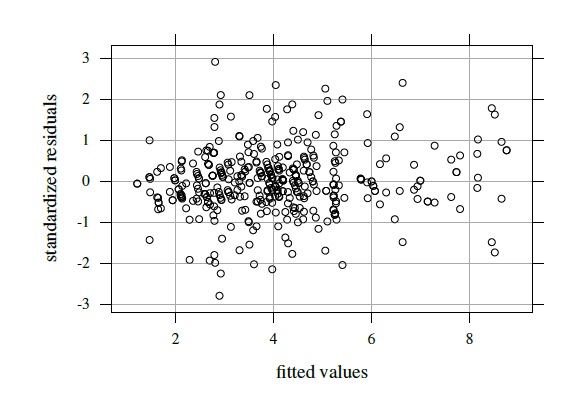
Figure 7.9 Residual plot for tumor size data.
7.10.2 Tumor Size Data
This dataset, introduced in Section 7.4, contains measurements of tumor sizes (in cm) of n = 40 lesions taken by five readers. Each measurement is repeated twice in an unlinked fashion. No reader serves as the reference and the interest is in all ![]() pairwise comparisons of the readers. The graphical displays in Figures 7.4, 7.5, and 7.7 show that the readers have the same scale and their correlation is moderately high, but they have somewhat different means and have considerable within-subject variation. There is also subject × reader interaction and the data appear homoscedastic.
pairwise comparisons of the readers. The graphical displays in Figures 7.4, 7.5, and 7.7 show that the readers have the same scale and their correlation is moderately high, but they have somewhat different means and have considerable within-subject variation. There is also subject × reader interaction and the data appear homoscedastic.
Figure 7.9 shows the residual plot that results from fitting the model (7.4). It does not show any trend and the vertical scatter appears constant. Besides, the normality of random effects and errors appear reasonable (Exercise 7.10). These suggest that the model fits well. Table 7.4 summarizes estimates of the 16 model parameters. From (7.9), we obtain the means and variances for the fitted normal distribution of (Y1,. ..,Y5) as (4.03, 3.59, 4.34, 4.27, 4.11) and (2.53, 2.96, 2.69, 2.49, 2.48), respectively, and 2.30 as the common covariance. The pairwise correlations range from 0.82 to 0.93. Reader 2 has the smallest mean and the largest variance.
Table 7.5 presents 95 % simultaneous confidence intervals for the ten pairwise bias differences. The critical points for these intervals is 2.706. None of the four intervals involving reader 2 covers zero. The interval for reader pair (1, 2) lies below zero while the other three lie above zero. This confirms reader 2 to have the smallest mean. Her/his estimated mean difference is the smallest (0.43) with reader 1 and is the largest (0.74) with reader 3. The remaining six intervals that do not involve reader 2 either cover zero or miss it by a whisker, implying that all other readers have practically the same means. The simultaneous intervals for precision ratios are not presented but the value of 1 is deep inside all the intervals. This suggests every reader has equal within-subject variations. However, a different picture emerges when we consider modified precision ratios given by (7.24) that include subject × reader interactions in the comparison. The 95 % simultaneous confidence intervals are presented in Table 7.5. The critical point for these intervals on the log scale is 2.725. Three intervals involving reader 2 do not cover 1. They show that the modified precision of reader 2 is substantially lower than those of readers 1, 4, and 5. The other intervals cover 1, implying similar pairwise precisions. On the whole, this similarity evaluation essentially confirms the deviant behavior of reader 2 in terms of both means and modified precisions.
Table 7.4 Summary of parameter estimates for tumor size data.
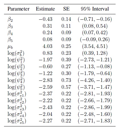 |
Table 7.5 Estimates and 95% simultaneous confidence intervals for all-pairwise bias differences and modified precision ratios for tumor size data.
| Pair | Bias Difference (βl − βj) | Precision Ratio |
||
| (j, l) | Estimate | 95% Interval | Estimate | 95% Interval |
| (1, 2) | −0.43 | (−0.81, −0.05) | 0.36 | (0.15, 0.84) |
| (1, 3) | 0.31 | (0.00, 0.62) | 0.61 | (0.24, 1.54) |
| (1, 4) | 0.24 | (0.01, 0.48) | 1.23 | (0.50, 3.06) |
| (1, 5) | 0.08 | (−0.16, 0.32) | 1.31 | (0.50, 3.39) |
| (2, 3) | 0.74 | (0.33, 1.16) | 1.70 | (0.72, 4.04) |
| (2, 4) | 0.67 | (0.31, 1.04) | 3.46 | (1.45, 8.30) |
| (2, 5) | 0.51 | (0.15, 0.88) | 3.67 | (1.41, 9.58) |
| (3, 4) | −0.07 | (−0.36, 0.23) | 2.04 | (0.81, 5.12) |
| (3, 5) | −0.23 | (−0.52, 0.07) | 2.16 | (0.89, 5.21) |
| (4, 5) | −0.16 | (−0.38, 0.05) | 1.06 | (0.41, 2.74) |
Table 7.6 presents 95% one-sided individual confidence bounds for repeatability versions of CCC and TDI (0.90 ) for each reader. The critical point for the CCC intervals on the Fisher’s z-scale is −1.645 and it is 1.645 for the TDI intervals on the log scale. Although on both measures reader 4 is the least and reader 3 is the most consistent, all readers have somewhat similar repeatability characteristic from a practical viewpoint. They have high reliabilities, as evidenced by the CCC estimates. However, the TDI bounds ranging from 0.8 to 1.0 are about 20–25% of ![]() , indicating relatively weak intra-reader agreement.
, indicating relatively weak intra-reader agreement.
Table 7.6 Estimates and one-sided 95% individual confidence bounds for repeatability versions of CCC and TDI (0.90) for tumor size data.
| Reader | CCCj | TDIj | ||
| j | Estimate | 95% Lower Bound | Estimate | 95% Upper Bound |
| 1 2 |
0.963 0.963 |
0.939 0.941 |
0.71 0.77 |
0.86 0.92 |
| 3 | 0.967 | 0.947 | 0.69 | 0.83 |
| 4 | 0.948 | 0.914 | 0.84 | 1.01 |
| 5 | 0.958 | 0.931 | 0.75 | 0.90 |
Table 7.7 presents 95% one-sided simultaneous confidence bounds for all-pairwise values of CCC and TDI (0.90). The critical point used in the CCC intervals on the Fisher’s z-scale is −2.250 and the same for the TDI intervals on the log scale is 2.464. The bounds range from 0.59 to 0.86 for CCC and from 1.26 to 2.56 for TDI. Remarkably, the bounds for both measures induce the same ordering of reader pairs on the basis of extent of agreement. In particular, the pair (2, 3) has the least agreement whereas the pair (4, 5) has the most. But even the highest level of agreement does not seem high enough to be deemed satisfactory. It is also apparent from the evaluation of similarity and repeatability that the relatively high error variation of the readers is a key cause of their poor agreement. It may be possible to reduce this error variation and hence improve the readers’ agreement by providing uniform training in determining the tumor sizes. The training may also correct the deviant performance of reader 2.
Table 7.7 Estimates and 95% one-sided simultaneous confidence bounds for all-pairwise values of CCC and TDI (0.90) for tumor size data.
| Pair | CCCjl | TDIjl | ||
| (j, l) | Estimate | 95% Lower Bound | Estimate | 95% Upper Bound |
| (1, 2) | 0.811 | 0.683 | 1.71 | 2.14 |
| (1, 3) | 0.866 | 0.770 | 1.39 | 1.71 |
| (1, 4) | 0.905 | 0.832 | 1.14 | 1.40 |
| (1, 5) | 0.917 | 0.852 | 1.06 | 1.30 |
| (2, 3) | 0.743 | 0.593 | 2.07 | 2.56 |
| (2, 4) | 0.780 | 0.640 | 1.87 | 2.33 |
| (2, 5) | 0.807 | 0.679 | 1.72 | 2.16 |
| (3, 4) | 0.888 | 0.807 | 1.25 | 1.53 |
| (3, 5) | 0.882 | 0.794 | 1.29 | 1.61 |
| (4, 5) | 0.921 | 0.859 | 1.03 | 1.26 |
7.11 CHAPTER SUMMARY
- The methodology for data on two methods is extended to more than two methods.
- It allows ANOVA-style multiple comparisons of method pairs, for example, all-pairwise comparisons or comparisons with a reference, on the basis of measures of pairwise similarity and agreement.
- The approach involves extending models for data on two methods to allow J methods in a straightforward manner, and performing simultaneous inference on measures of pairwise similarity and agreement for method pairs of interest.
- For unreplicated data, the model (4.1) is extended. In this extension, the usual problems in estimation of variance components do not arise.
- For repeated measurements data, the models (5.1) and (5.9) for unlinked and linked data are generalized. By default, the variances for subject × method interactions are assumed to be unequal, but one can assume equal variances if needed.
- The methodology can be further extended to allow heteroscedasticity of errors along the lines of Chapter 6.
- As before, the methodology assumes that all the methods are on the same scale and the number of subjects is large.
7.12 TECHNICAL DETAILS
For paired measurements data, recall that the mixed-effects model (4.1) is written in the usual matrix form as (4.15). To write its extension (7.1) for unreplicated data on J (≥ 2) methods in the same form, define

Expand the vectors and matrices in (4.14) as

With this notation, the model (7.1) for i = 1,...,n can be written as
 (7.34)
As before, this implies Yi ∼NJ (Xβ, V = ZGZT + R), where the mean vector Xβ and the covariance matrix V yield the expressions in (7.2) upon using the fact that β1 = 0. The vector of transformed parameters is

For unlinked repeated measurements data, we similarly expand the notation in (5.38) and (5.39) for two methods to accommodate J (> 2) methods. This involves taking
 (7.35)
The model (7.4) for i = 1,...,n can now be written as

It follows that
where the elements of the mean vector Xiβ and the covariance matrix Vi are given earlier in (7.5)–(7.7) (Exercise 7.3). The vector of transformed parameters of this model is

For linked repeated measurements data, Yi, ei, Xi, and Ri are the same as for unlinked data with (mij, Mi) = (mi, Jmi). But the random effects vector ui is a ![]() -vector
-vector
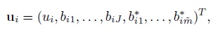
its covariance matrix G is a ![]() ×
× ![]() diagonal matrix
diagonal matrix

and the design matrix Zi associated with ui is an appropriately defined Mi × ![]() matrix of ones and zeros, with
matrix of ones and zeros, with ![]() as in Section 5.9. Now the model (7.14) for i = 1,...,n can be written as
as in Section 5.9. Now the model (7.14) for i = 1,...,n can be written as
implying
The elements of the mean vector and covariance matrix here are given in (7.15)–(7.18) (Exercise 7.5). The vector of transformed parameters of this model is

The models in this chapter can be fit by the ML method using a statistical software that handles mixed-effects models. We proceed as in Chapter 3 for the estimation of various measures, computation of standard errors of the estimates, and construction of individual as well as simultaneous confidence intervals and bounds.
7.13 BIBLIOGRAPHIC NOTE
Many of the papers cited in previous chapters for two methods, especially those dealing with CCC and modeling of data, actually contain extensions for multiple methods. The CCC-focussed articles include Lin (1989), King and Chinchilli (2001a), Barnhart et al. (2002), Carrasco and Jover (2003), Barnhart et al. (2005), and Lin et al. (2007). The modeling articles include Carstensen et al. (2008) and Schluter (2009). The papers on CCC summarize the overall level of agreement among the multiple methods in a single index by either taking a weighted average of the pairwise CCCs or replacing the moments in the definition of CCC by their weighted averages taken over the method pairs. In principle, such an approach can be used with other measures of similarity and agreement as well. However, we find such overall measures difficult to interpret and prefer to keep the pairwise measures separate and perform simultaneous inference on them. Unlike the overall measures, the separate pairwise measures allow us to directly compare the method pairs on the basis of extent of similarity or agreement and also to determine which pairs are similar or agree well, while adjusting for multiplicity of inferences.
The approach based on simultaneous inference on pairwise measures is inspired by the multiple comparisons of means in ANOVA for which the monograph by Hsu (1996) is a good reference. This approach has been taken by Hedayat et al. (2009) and Choudhary and Yin (2010). The first article works with unreplicated multivariate normal data and focuses on coverage probability as the agreement measure, which has one-to-one correspondence with TDI (Chapter 2). It develops simultaneous confidence bounds for pairwise values of the measure and a test of homogeneity for them. The second article works with unreplicated as well as repeated measurements data assumed to follow a mixed-effects model. It develops frequentist and Bayesian procedures for simultaneous bounds on pairwise values of any scalar agreement measure. This is also the basis for some of the material in this chapter. The models here are similar, but not identical, to those in Carstensen et al. (2008).
The critical points used in the simultaneous confidence bounds and intervals are computed using the multcomp package of Hothorn et al. (2008) in R.
St. Laurent (1998), Hutson et al. (1998), and Harris et al. (2001) assume a “gold standard” method in the comparison that serves as a reference. The comparisons with a reference can be accommodated in the multiple comparisons approach of this chapter.
Data Sources
The systolic blood pressure data are from Barnhart et al. (2002). Broemeling (2009, Chapter 6) is the source of the tumor size data and contains further details about them.
EXERCISES
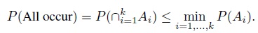
- (Bonferroni Inequality) Let A1 ,A2,...,Ak be k events. Show that
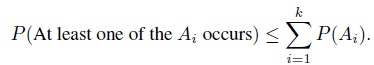
- For the events in part (a), show that
- For i = 1, ..., k, let Ii be a 100(1 − α)% confidence interval for parameter θi; and Ei = {θi ∈ Ii} be the event that the interval Ii covers the true parameter θi. Then, by definition, the coverage probability of the ith interval is P(Ei) ≥ 1 − α. Use parts (a) and (b) to show that the simultaneous coverage probability of the k intervals satisfies the inequalities

- Deduce from part (c) that if each Ii is a 100(1 − α/k)% confidence interval, then the k intervals together form a set of 100(1 − α)% simultaneous confidence region for θ1,...,θk that is generally conservative.
- (Bonferroni Inequality) Let A1 ,A2,...,Ak be k events. Show that
- Under the model (7.1), show that the marginal distribution of (Yi1,...,Yij) on subject i is given by (7.2) for i = 1,...,n.
- This is a generalization of Exercise 5.1 for J (> 2) methods. Show that the marginal distribution of the vector Yi of unlinked observations on subject i is given by (7.36) for i =1 ,...,n. Show also that the elements of the mean vector and covariance matrix of Yi are given by (7.5)–(7.7).
- This is a generalization of Exercise 5.2 for J (> 2) methods. Consider the model (7.4) for unlinked repeated measurements data, and also the companion models for Yj and
 (j = 1,...,J) given by (7.8) and (7.11).
- This analog of Exercise 7.3 for linked data is a generalization of Exercise 5.3 for J (> 2) methods. Show that the marginal distribution of the vector Yi of linked observations on subject i (i = 1,...,n) is given by (7.38). Show also that the elements of the mean vector and covariance matrix of Yi are given by (7.15)–(7.18).
- This analog of Exercise 7.4 for linked data is a generalization of Exercise 5.4 for J (> 2) methods. Consider the model (7.14) for linked repeated measurements data.
- Show that the marginal distribution of (Y1,. ..,YJ) is a J-variate normal distribution with mean vector and covariance matrix given by (7.19) and (7.20). Verify the distribution of Djl given in (7.21).
- Show that the marginal distribution of (Yj, ) is given by (7.22) for j = 1,..., J. Deduce the distribution of Dj given in (7.23).
- Confirm the expressions for agreement measures given in (7.25), (7.26), and (7.27).
- Verify the expressions for repeatability measures given in (7.30) and (7.31).
- Fractional area change is measured in 15 subjects in an echocardiographic imaging study using four methods—a fuzzy gold standard (FGS) derived from a consensus of experts, two distinct echocardiographers (EXP1 and EXP2), and an automatic boundary detection (ABD) algorithm, which requires no observer input. Table 7.8 presents the data. As there is a reference method in the study, the comparisons with the reference are of interest.
Table 7.8 Fractional area change measurements (in %) for Exercise 7.9.
Method Subject FGS EXP1 EXP2 ABD 1 41.25 26.96 45.96 26.78 2 37.95 39.87 36.95 26.88 3 37.23 31.69 31.72 39.08 4 40.62 36.41 30.58 24.63 5 34.67 44.77 40.55 39.82 6 32.31 31.46 33.03 28.53 7 28.53 35.13 10.97 28.84 8 39.25 40.69 33.10 39.06 9 35.37 33.93 34.85 30.24 10 40.17 43.99 38.72 34.77 11 38.53 22.86 31.07 42.43 12 36.39 40.99 26.34 34.48 13 40.82 32.78 34.61 34.21 14 37.52 24.09 29.65 25.69 15 42.01 51.99 42.00 37.03 Reprinted from Hutson (2010), ©2010 Elsevier, with permission from Elsevier.
- Perform an exploratory analysis. Do the methods appear to have the same scale? Do you notice any outliers? If yes, how would you deal with them?
- Fit model (7.1) to the data. Check adequacy of the model assumptions.
- Evaluate similarity between fuzzy gold standard and other methods.
- Evaluate agreement between fuzzy gold standard and other methods. Which of the methods can be used interchangeably with it?
- If outliers are seen, analyze the data again after removing them, and compare the conclusions.
- Consider the tumor size data from Section 7.10.2.
- Fit model (7.4) to the data and verify the results in Tables 7.4–7.7.
- Perform model diagnostics to verify whether the normality assumption for errors and random effects appear reasonable.
- Standardized uptake value, a measure of lesion size, is measured in 20 lung cancer patients by three readers with the help of CT-PET imaging. Each measurement is replicated twice in an unlinked manner. The data are presented on page 202 of Broemeling (2009).
- Perform an exploratory analysis of the data with summary measures and graphical displays.
- Fit model (7.4) to the data. Are the unequal variances for patient × reader interactions estimated reliably? If not, fit a simpler model that assumes equal variances for the interactions.
- Check adequacy of the simpler model. Does the homoscedasticity assumption appear reasonable? If not, is this assumption reasonable for the log-transformed data? Find an adequate model for the data either on the original scale or on the transformed scale.
- Evaluate repeatability of each reader.
- Evaluate similarity of all reader pairs.
- Evaluate pairwise agreement between all readers. Do the readers agree well?
- Bland and Altman (1999) report a study where two observers and an automatic blood pressure measuring machine simultaneously measure systolic blood pressure. Each makes three observations in quick succession on 85 subjects. We assume the repeated measurements to be unlinked. The data can be obtained from the book’s website.
- Fit model (7.4) to these data. Examine the estimates of variance components and judge whether they can be considered reliable.
- Fit the following modification of (7.4) to these data:
where βj are unknown intercepts; the random effects (bi1, bi2, bi3) are i.i.d. draws from a trivariate normal distribution with zero mean and an unstructured covariance matrix; and the errors follow independent
 distributions, independently of the random effects. Perform model diagnostics to check goodness of fit of the model. Comment specifically on the normality assumption for random effects and errors.
 - Evaluate similarity and agreement using the model fit in part (b).