CHAPTER 1
INTRODUCTION
1.1 PREVIEW
This chapter focuses on method comparison studies involving two methods of measurement of a quantitative variable. It introduces the companion problems of evaluation of similarity and evaluation of agreement between the methods, reviews the related concepts, critically examines the currently popular statistical tools, and describes a model-based approach for data analysis. It also points out the inadequacy of the widely used paired measurements design for data collection for the purpose of measuring agreement. To keep the flow of the text smooth, specific references are provided in the bibliographic note section at the end of the chapter. This practice is followed throughout the book.
1.2 NOTATIONAL CONVENTIONS
We generally use uppercase roman letters for random quantities whose values can be observed, for example, measurements made by medical devices. Lowercase roman letters are generally used for random quantities whose values cannot be observed (e.g., measurement errors) and for observed values of observable random quantities. Vectors and matrices are denoted by boldface letters. Their dimensions are clear from the context. By default, a vector is a column vector, and its transpose is denoted by attaching the superscript T to its symbol. For example, x is a column vector, xT is the transpose of x, and X is a matrix. We also use I for an identity matrix, 1 for vectors and matrices of ones, and 0 for vectors and matrices of zeros. We often attach a subscript to these symbols for clarity. For example, In denotes an n × n identity matrix and 1n denotes an n × 1 vector of ones. A diagonal matrix is denoted as diag {x1,..., xn}. If A 1,..., An are matrices, diag {A1,..., An} denotes a block-diagonal matrix. Further, tr(A), |A|, and A −1, respectively, denote the trace, determinant, and inverse of a (square) matrix A.
Generally, the unknown scalar and vector parameters are denoted by lowercase Greek letters. An exception to this rule is the letter α, which is used as a known level of significance of a test of hypothesis and 100(1 − α)% represents level of confidence of a confidence interval or bound. Matrices of unknown parameters as well as known quantities (e.g., the design or the regression matrix) are denoted by uppercase roman letters in boldface. A “hat” over an unknown parameter denotes its estimate, whereas a “hat” over a random quantity denotes its predicted or fitted value. The (estimated) standard error of the estimator ![]() of an unknown parameter θ is denoted by SE(
of an unknown parameter θ is denoted by SE(![]() ).
).
We also use the convention that if, say, Y is a random quantity, then Y1,Y2,... denote observations from the distribution of Y. Similarly, if Yj is a random quantity, then Yij, i ≥ 1, denote observations from the distribution of Yj.
We use N1(µ, σ2) for a univariate normal distribution with mean µ and variance σ2. A multivariate normal distribution having p components with mean vector µ and covariance matrix V is denoted as Np(µ, V). We also use zα, tk, α, χ2k, α and fk1,k2,α to, respectively, denote the (100α) th percentiles of a N1(0, 1) distribution, a t distribution with k degrees of freedom, a χ2 distribution with k degrees of freedom, and an F distribution with k1 and k2 as numerator and denominator degrees of freedom, respectively. We further use χ2k,α(δ) and tk,α(δ), respectively, to denote the (100α) th percentiles of noncentral χ2 and t distributions with k degrees of freedom and noncentrality parameter δ. Finally, log refers to natural logarithm throughout the book.
1.3 BASIC CHARACTERISTICS OF A MEASUREMENT METHOD
Measurements are fundamental to any scientific endeavor. In particular, in health-related fields, measurements of clinically important quantities form the basis of diagnostic, therapeutic, and prognostic evaluation of patients. The quantity being measured may be continuous (or quantitative), for example, level of cholesterol, blood pressure, and concentration of a chemical. The quantity may also be categorical (or qualitative), for example, presence or absence of a medical condition and severity of a disease as identified by stage. Although this chapter is concerned with continuous measurements, it is obvious that any measurement process is prone to errors, regardless of whether its outcome is continuous or categorical. The errors in measurement cause the observed values to differ from the true underlying values. The relationship between the observed and the true values can be studied using statistical models.
Before describing such a model, let us set up some notation. Let the random variable Y represent the observed measurement from a method of measurement on a randomly selected subject from a population. We use the term “measurement method” in a generic sense. It may refer, for example, to an instrument, an assay, a medical device, a technician, or a clinical observer. The term “subject” is used here to refer to the entity on which the measurements are taken. For example, it may be a patient, a specimen, or a blood sample. Next, let the random variable b denote the true measurement of the subject associated with Y. The true value is well defined, albeit it may be hard to measure directly (e.g., blood pressure); or it may be unobservable. In either case, the true value is not observed; and it is treated like a latent variable or a random effect.
1.3.1 A Statistical Model for Measurements
A commonly used model relating the observed Y to the true b is the classical linear model. It assumes
 (1.1)
(1.1)where β0 and β1 are fixed constants specific to the measurement method; and e is the random error of the method. The following assumptions are also made:
(i) The true value b has a probability distribution over the population of subjects. This b distribution has mean (or expected value) µb and variance σb2. The variance σb2 is called the between-subject variance as it represents subject to subject variability in the true values—that is, the heterogeneity in the population.
(ii) The error e has a probability distribution with mean zero and variance σe2. This distribution is over replications of the same underlying measurement by the same method on the same subject under identical conditions. For this reason, the error variance σe2 is also called the within-subject variance. The square root of this variance is often known as the repeatability standard deviation or the analytical standard deviation of the measurement method.
(iii) The distributions of errors and true values are independent.
This model assumes that the error variance remains constant throughout the range of the value being measured. Often, this is not the case as the error variance may depend on the magnitude of measurement. An extension of the above model that accommodates such heteroscedastic errors is presented in Chapter 6.
A distinction is made between the true value of the subject and the true (i.e., error-free) value of the measurement method. The true value of the subject is b, whereas the true value produced by the measurement method is β0 + β1 b. These true values are linearly related in our model.
1.3.2 Quality Characteristics
The intercept β0 in the model (1.1) is called fixed bias of the measurement method. It is a constant that the method adds to its measurements regardless of the true value being measured. The slope β1 is called proportional bias or level-dependent bias. Instead of correctly measuring the true b, the method measures it as β1 b. In other words, β1 is the amount of change observed by the method if the true b changes by 1 unit. Both the fixed bias β0 and the proportional bias β1 cause systematic errors in measurement.
Under the model (1.1), the conditional mean and variance of Y given b are
 (1.2)
(1.2)respectively. These quantities essentially represent the average and the variance of an infinitely large number of replications produced by the method while evaluating the same subject under identical conditions. The conditional mean is also what we have called the error-free value of the method.
A measurement method is said to be accurate if it has no bias in estimating the true value b. The biases β0 and β1 measure the magnitude of the lack of accuracy of the method. Consequently, a method is accurate if (β0, β1) = (0, 1). In this case, the method has neither fixed nor proportional bias and its error-free value always matches the true value. Turning this interpretation around, we can say that the true value of a subject is the average of a large number of replications made on the subject under identical conditions by a method that has no bias.
The precision of a measurement method is related to the size of the random errors in The variance σe2 of these errors measures variability in the observed Y around the error-free value of the method. Thus, σe2 is a measure of the precision of the method and sometimes is formally defined as the reciprocal of the error variance. The method is fully precise if σe2 =0. In this case, the method has no measurement error—its observed value equals its error-free value.
A measurement method may appear highly precise merely because it is too crude to discern small changes in the true value. The ability of a method to discern small changes is measured by a relative measure of precision known as sensitivity. The notion of sensitivity combines the rate of change and the precision of a measurement method in a single index. For the model (1.1), it is given by |β1|/σe. To understand the motivation behind this index, recall that the slope β1 represents the rate of change in the error-free measurement of the method with respect to the true b. Thus, if |β1| is large, a small change in b will cause a comparatively large change in its measured value, resulting in increased sensitivity. Also, if the error variance is small, the observed measurement Y will be precise and the sensitivity will be large. In either case, it will be relatively easy to distinguish b from its nearby values on the basis of the observation Y. The larger the sensitivity, the more effective is the measurement method. Often when the interest is in comparing two methods, the square of the sensitivity is considered the precision of a method (Section 1.7.1).
It can be seen that the marginal mean and variance of Y are (Exercise 1.1)
 (1.3)
(1.3)respectively. These quantities represent the average and variance of the measurements in the population from which the subject is being sampled. The expression for the variance also shows that there are two sources of variation—the true values in the population and the random errors. The variance is also affected by the proportional bias (β1) of the method.
The reliability of a measurement method is defined as the proportion of variation in observed measurements that is not explained by the error variation inherent in the method. The reliability of a method following the model (1.1) is
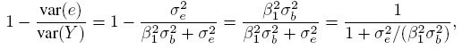 (1.4)
(1.4)where the variance of Y is substituted from (1.3). It can also be interpreted as the correlation between two independent replications of the same underlying measurement (Exercise 1.1). Thus, the reliability is actually an intraclass correlation. It ranges between zero and one. It increases as the error increases as the error variance σe2 decreases in relation to the variance β21 σb2 in the errorfree measurements. This way the reliability of a method is a measure of its relative precision. A high value of reliability indicates that the error variation is small compared to the variation in the error-free values.
The expression for reliability shows that it depends on the error variation of the method as well as the heterogeneity (or the between-subject variation) in the population. In particular, the reliability increases as the population heterogeneity increases even if the precision of the method does not change. Thus, care must be taken in interpreting reliability.
1.4 METHOD COMPARISON STUDIES
Method comparison studies are designed to compare two competing methods of measurement of the same quantity, having a common unit of measurement. The measurements are taken by each method on every subject in the study, and there may or may not be replications. In this book, we are primarily concerned with the case when the methods under consideration are assumed to be fixed rather than a random sample from a population of methods. The case of randomly selected methods providing categorical measurements is discussed in Chapter 12.
A distinguishing feature of method comparison studies is that none of the methods in the study is assumed to be producing the true values. The true values remain unknown and the methods involved measure them with error. Usually, one of the methods is a new test method and other is an established standard method, which is often called the gold standard or the reference method. However, the gold standard designation does not mean that the method is free of systematic and random errors. It is also understood that future improvements in the measurement technique may render a current gold standard obsolete.
Generally, there are two goals for a method comparison study. The primary one is to quantify the extent of agreement between the measurement methods and determine whether they have sufficient agreement so that we can use them “interchangeably” for a particular purpose. By interchangeable use we mean that a measurement from one method on a subject can be replaced by a measurement from another method without causing any difference in the practical use of the measurement. In other words, it does not matter which method is being used to take the measurement as both give practically the same value. If two methods agree well enough to be used interchangeably, we may prefer the one that is cheaper, faster, less invasive, or is simply easier to use. This is also the motivation behind method comparison studies.
A secondary goal of a method comparison study is to compare characteristics of the measurement methods—such as their biases, precisions, and sensitivities—to find the differences in the methods that cause them to disagree. We refer to this comparison as evaluation of similarity. Understanding why the methods disagree is important. For example, we may discover that a new method does not agree well with a standard method because it is much more precise than the standard method.
The two putative goals of a method comparison study—evaluation of agreement and evaluation of similarity—are closely related. For example, when the methods agree well, it generally implies that their characteristics are similar as well. Likewise, when one method is substantially more precise than the other or when the methods have quite different characteristics, the issue of agreement evaluation may be moot. However, the methods may not agree well despite having similar characteristics. Furthermore, when the methods do not agree well, a comparison of their characteristics reveals why the methods disagree. This information is helpful in determining whether one method is clearly superior to the other. It may also suggest corrective actions that may improve the extent of agreement between the methods. Often, a simple addition of a constant to one method or its rescaling may be all that is needed.
A method comparison study may seem similar to a calibration study, but their goals are different. In a typical calibration study, subjects with known measurements of a variable obtained from a highly accurate method that has negligible measurement error are also measured by a test method to develop an equation that converts a measurement from the test method into a predicted true measurement. In contrast, in a method comparison study, the methods being compared are already calibrated. Although there may be a standard method in the comparison, it is not assumed to be error free. If, however, the methods do not agree well, then an equation may be developed to transform measurements from one method for better agreement with the other.
1.5 MEANING OF AGREEMENT
To fix ideas, assume that the two methods are labeled as “1” and “2.” Let Y1 and Y2, respectively, denote the paired measurements from methods 1 and 2 on a randomly selected subject from the population. It may be helpful to think of (Y1,Y2) as paired measurements on a typical subject. We assume that (Y1,Y2) has a continuous bivariate distribution with mean (µ1, µ2), variance (σ1 = σ12, σ22), covariance σ12, and (Pearson or product-moment) correlation ρ. The correlation is typically positive in practice. Let D = Y2 − Y1 denote the difference in the measurements. It follows a continuous distribution with mean ξ = µ2 − µ1 and variance τ22 = σ21+ σ22 − 2 ρσ1 σ2.
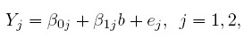
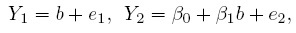
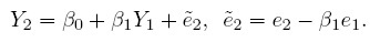
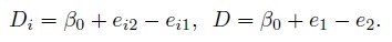
Agreement between two methods refers to closeness between their measurements. The methods have perfect agreement in the ideal case when P(Y1 = Y2)= 1. In this case, the bivariate distribution of (Y1, Y2) is concentrated on the line of equality—the 45◦ line, causing the distribution of the difference to be degenerate at zero. This will be reflected in the scatterplot of Y2 versus Y1 if all (Y1, Y2) values fall on the line of equality. See panel (a) of Figure 1.1 for such a scatterplot of simulated data. In this case, all the differences are zero. Thus, perfect agreement corresponds to any of the following two equivalent conditions (Exercise 1.2):
(i) ![]() that is, the methods have equal means, equal variances, and correlation one, or
that is, the methods have equal means, equal variances, and correlation one, or
(ii) ![]() that is, the difference has zero mean and zero variance.
that is, the difference has zero mean and zero variance.
However, it is unrealistic to expect this ideal condition to hold in practice and some deviation from perfect agreement is inevitable. In fact, some degree of lack of agreement is acceptable as this is the very premise of a method comparison study.
The notion of perfect agreement is quite restrictive. For example, the methods may have equal means (ξ = 0). But this may not be enough for good agreement because the two variances may differ considerably, causing unacceptably large variability in the differences around zero (i.e., large τ2) even when the correlation between the measurements is high. Having equal variances in addition to equal means may also not be enough for good agreement because if the correlation is small, one would again obtain a large τ2. (Recall from Exercise 1.2 that τ2 = 0 if and only if σ21 = σ22 and ρ =1.) Moreover, the methods may have poor agreement despite having a perfect correlation (ρ = ±1) as it is a necessary but not sufficient condition for perfect agreement. This happens because the correlation is a measure of linear relationship, not of agreement. A perfect linear relationship simply means ![]() where
where ![]() are constants. In this case,
are constants. In this case, ![]() and
and ![]() Thus, depending upon how far away
Thus, depending upon how far away ![]() is from zero and
is from zero and ![]() is from one, the methods may have substantially different means and variances, implying large ξ and τ2, and hence poor agreement. See panels (b)–(d) of Figure 1.1 for scatterplots of simulated data for the following scenarios: unequal means but equal variances, equal means but unequal variances, and nearly perfect correlation but unequal means and unequal variances.
is from one, the methods may have substantially different means and variances, implying large ξ and τ2, and hence poor agreement. See panels (b)–(d) of Figure 1.1 for scatterplots of simulated data for the following scenarios: unequal means but equal variances, equal means but unequal variances, and nearly perfect correlation but unequal means and unequal variances.
For a familiar example of perfect correlation but poor agreement, consider measuring temperature using a thermometer calibrated in Celsius (method 1). Take method 2 as the method that simply transforms the method 1 measurements into Fahrenheit, that is, Y2 = 32+(9 /5) Y1. These two methods are perfectly correlated, but they obviously have poor agreement. Nevertheless, in this case a simple recalibration of method 2 as 5(Y2 − 32) /9 will make the methods agree perfectly.
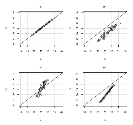
Figure 1.1 Scatterplots of simulated paired measurements data with high correlations superimposed with the line of equality. (a) The methods have perfect agreement. (b) The methods have unequal means but equal variances. (c) The methods have unequal variances but equal means. (d) The methods have unequal means and variances.
If the notion of agreement appears unduly restrictive, recall that some deviation from perfect agreement is acceptable provided the deviation is not too large to prohibit interchangeable use of the methods. Essentially, this means that some difference in means and variances and a non-perfect correlation is acceptable as long as the methods can be considered to have sufficient agreement for the intended purpose.
To evaluate agreement, we do two things. First, we quantify the extent of agreement by measuring how far the paired measurements are from the line of equality. The measures of agreement are used for this purpose. They are specific functions of parameters of the bivariate distribution of (Y1, Y2) and perfect agreement corresponds to appropriate ideal boundary values for these measures. Some common agreement measures are described in Chapter 2. Second, we determine whether the agreement is sufficiently strong to justify interchangeable use of the methods for the purpose at hand. This can be done by comparing the observed value of the agreement measure to a threshold value that represents acceptable agreement. The threshold, however, depends upon the intended use of the measurement and has to be clarified on a case-by-case basis. It is entirely possible for the methods to agree while both being wrong.
1.6 A MEASUREMENT ERROR MODEL
To explain how the notion of agreement is related to the characteristics of the two methods, we first need a model that links the observed (Y1,Y2) to the true value being measured and the measurement errors associated with the methods. It is common to assume the classical model (1.1) that leads to the following setup for the bivariate data:
 (1.5)
(1.5)where the intercept β0j is the fixed bias of the j th method; the slope β1j is its proportional bias; and ej is its measurement error. As before, b is the true measurement of the subject. The assumptions regarding b are the same as those for model (1.1). The error ej is assumed to have a mean of zero and variance σ2ej that depends on the method. The errors are mutually independent of each other and of the true value. Later, the errors and the true values will be assumed to follow normal distributions (see Section 1.12); but these distributional assumptions are not needed at this time.
In this model, the error-free values of the methods, namely, β01 + β11b and β02 + β12 b, are linearly related to the true underlying value, and hence are linearly related to each other. This relationship between the error-free values induces dependence in the observed Y1 and Y2 since they share the common b, which itself is a random variable. However, conditional on b, Y1 and Y2 are independent.
When the two methods have different proportional biases, that is, β11 ≠ β12, we can interpret the situation as the methods having different measurement scales. This means that a unit change in the true value of the subject does not cause equal change in error-free values of both methods. As a result, the difference in the error-free values, β02 − β01 +(β12 − β11) b, is not a constant. Methods with different scales also have unequal variabilities in their error-free values ![]() The terms “difference in proportional biases” and “difference in scales” are used interchangeably in this book.
The terms “difference in proportional biases” and “difference in scales” are used interchangeably in this book.
Familiar examples of methods with obviously different scales include thermometers calibrated in Fahrenheit and Celsius, and weighing scales calibrated in ounces and grams. Although in both these examples, the units of measurement are also different, it may happen that methods have different scales despite having a common nominal unit (Section 1.8).
1.6.1 Identifiability Issues
Although so far we have called b as the true measurement, the absolute truth is not available in most method comparison studies. Under our model assumptions, the true value is identifiable only up to a linear transformation. This is because the same linear model (1.5) results if b in (1.5) is replaced by its linear transformation ![]() are redefined as
are redefined as ![]() The practical implication of this lack of identifiability is that the method-specific fixed and proportional biases cannot be determined. As a result, we cannot evaluate how close β0j is to zero or β1j is to one, meaning that we cannot ascertain how accurate the j th method is. With appropriate data, however, we can determine how close the bias differences β02 − β01 and β12 − β11 are to zero. This serves the purpose of method comparison because we are generally not interested in determining how accurate the individual methods are, but rather in comparing the methods and evaluating their agreement.
The practical implication of this lack of identifiability is that the method-specific fixed and proportional biases cannot be determined. As a result, we cannot evaluate how close β0j is to zero or β1j is to one, meaning that we cannot ascertain how accurate the j th method is. With appropriate data, however, we can determine how close the bias differences β02 − β01 and β12 − β11 are to zero. This serves the purpose of method comparison because we are generally not interested in determining how accurate the individual methods are, but rather in comparing the methods and evaluating their agreement.
We can resolve the identifiability problem by assuming, without any loss of generality, that one of the methods (say, method 1) is the reference method and setting β01 = 0 and β11 = 1. This leads to the simplified model
 (1.6)
(1.6)where, for notational convenience, we have replaced (β02, β12) by (β0, β1). Note that it does not matter which method is tagged as the reference method; but if there is a gold standard, it makes sense to use it as the reference. The concept of a reference method is needed just to enforce identifiability.
This model offers a working definition of the true measurement as well. Since from (1.6), E(Y1| b) = b, the true value is what the reference method measures on average. In other words, the true value is the error-free value of the reference method. However, we cannot say whether this method is accurate. Moreover, the intercept β0 in the model (1.6) represents the difference in the fixed biases of the methods. When β0 = 0, the methods have the same fixed bias. Similarly, a non-unit value of the slope β1 indicates a difference in the proportional biases (or scales) of the methods.
The model (1.6) is an example of a measurement error model. It is also called an errors-in-variable model because the model for Y2 can be interpreted as a linear regression model, where the covariate b on which Y2 is regressed is not observed directly. Instead, b is measured with error as Y1. In the parlance of measurement error models, (1.6) or a structural model or a structural equation model, as opposed to a functional model, because the true b is considered random.
To see how this model differs from the ordinary linear regression model of Y2 on Y1, substitute b = Y1 − e1 in the expression for Y2 to get
Despite a superficial similarity, this model is not the ordinary linear regression model because the explanatory variable Y1 and the error ![]() are not independent in this model, unless of course, Y1 is error free (i.e.,
are not independent in this model, unless of course, Y1 is error free (i.e., ![]() = 0 ).
= 0 ).
1.6.2 Model-Based Moments
The measurement error model (1.6) postulates that the paired measurements (Y1, Y2) follow a bivariate distribution with mean vector
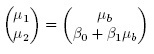 (1.7)
(1.7)and covariance matrix
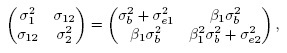 (1.8)
(1.8)see Exercise 1.3. Clearly, there are two factors that may lead to unequal means, viz., a nonzero β0 and a non-unit β1. Similarly, there are two factors that may cause unequal variances, viz., a non-unit β1 and unequal error variances. Further, the dependence in the bivariate distribution is solely due to the sharing of the common true value b by the two methods.
It follows from (1.8) that the (Pearson) correlation between Y1 and Y2 is
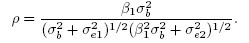 (1.9)
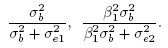
(1.9)From (1.4), this correlation can be interpreted as the square root of the product of the reliabilities of methods 1 and 2, given by
Thus, the correlation also depends on the between-subject variation in the population being measured. If the same methods are used in two populations—one with greater heterogeneity than the other—the methods would exhibit higher correlation in the population with greater heterogeneity. Due to this property, comparisons of such correlations need to take the population variability into account.
From (1.7) and (1.8), simple algebra shows that the mean and variance of the difference D = Y2 − Y1 are
 (1.10)
Thus, the effects of the difference in fixed biases and the difference in scales get confounded in the mean ξ. The difference in scales also contributes to the variance τ2.
1.6.3 Conditions for Perfect Agreement
From the model-based expressions for the moments of (Y1,Y2) and D given by (1.7)–(1.10), and the definition of perfect agreement from Section 1.5, it follows that the methods can have perfect agreement only when
Hence for perfect agreement, not only must the methods have equal fixed and proportional biases, but they must also have no measurement errors. In other words, any imprecision in either method or any difference in the fixed or proportional biases of the methods is a source of disagreement. Therefore, when we say that some lack of agreement is acceptable, we essentially mean that we are willing to tolerate some imprecision in the methods and some differences in their fixed and proportional biases. For good agreement, the differences in these biases and the measurement errors of both methods must be small.
Table 1.1 Interpretation of test theory terms in the context of method comparison studies under the measurement error model (1.6).
| Test Theory Term | Parameter Setting | Interpretation |
| essential tau-equivalence | β1 = 1 | equal proportional biases |
| tau-equivalence | (β0, β1) = (0, 1) | equal fixed and proportional biases |
| parallelism | (β0, β1,σ21) = (0, 1,σ2e2) | equal fixed and proportional biases, and equal precisions |
1.6.4 Link to Test Theory
If we refer to measurement methods as “tests” and measurements as “scores,” then the model (1.6) is known in psychometry as a test theory model. The tests following this model are called congeneric as their error-free scores, b and β0 + β1 b, are linearly related. The tests are called essentially tau-equivalent if β1 = 1. In this case, the error-free scores are measured on the same scale but they may differ by a constant. The tests are said to be tau equivalent if (β0, β1) = (0, 1). In this case, the tests have the same error-free scores or accuracy, that is, they have the same fixed bias and the same scale, but their precisions may be different. Further, the tests are said to be parallel if they are tau equivalent and σe12 = σe22. In this case, the tests not only have the same accuracy, but they also have the same precision. These connections between the concepts in method comparison studies and test theory are summarized in Table 1.1.
1.7 SIMILARITY VERSUS AGREEMENT
1.7.1 Evaluation of Similarity
The measurement error model (1.6) suggests that the two methods can be compared on the following characteristics of their marginal distributions:
- Fixed bias: The intercept β0 represents the difference in fixed biases of the methods. If β0 = 0, the methods have the same fixed bias.
- Scale (or proportional bias): The slope β1 indicates the difference in the scales of the methods. If β1 = 1, the methods have the same scale.
- Precision: The difference in the precisions of the methods can be measured by the precision ratio, defined as
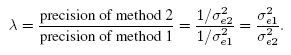 (1.11)
If λ = 1, the methods are equally precise, whereas if λ < 1, method 1 is more precise than method 2, and the converse holds if λ < 1.
- Sensitivity: The sensitivities of the methods (Section 1.3.2) can be compared using the squared sensitivity ratio, defined as
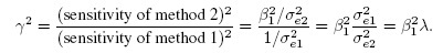 (1.12)
When γ2 < 1, method 1 is more sensitive than method 2, and the converse is true if γ2 > 1. The sensitivity metric γ2 is the product of precision ratio and squared ratio of proportional biases. Thus, when the methods have the same scale (i.e., proportional bias) and precision, they also have equal sensitivity (γ2 = 1).
The precisions of methods are comparable only when the methods have the same scale. For example, the precisions of two thermometers—one calibrated in Fahrenheit and another in Celsius—cannot be compared, unless one of them is transformed to have the same scale as the other. For methods following model (1.6), this transformation amounts to replacing Y2 with, Y2/β1, leading to σ2e2/β21 as the new error variance. This error variance is comparable to σ2e1, and the precision ratio comparing them results in y2. Thus, y2 is actually the precision ratio after rescaling one of the methods to have the same scale as the other. For this reason, the squared sensitivity is often called the “precision” of a method and is unaffected by the intercept β0.
To summarize, under model (1.6), the differences in the marginal characteristics of the methods are measured using β0, β1, λ, and γ2. These quantities are collectively called the measures of similarity. None of these measures involve any parameters of b the true quantity being measured. Therefore, the comparison of methods through these measures is unaffected by the properties of b such as its magnitude, variability, range, etc. This contrasts with measures of agreement that typically involve such parameters (see Section 1.5 and Chapter 2). Obviously, in the test theory language, parallelism is the best outcome we can expect when we evaluate similarity of two methods.
1.7.2 Evaluation of Agreement
Evaluation of similarity is essentially a comparison of marginal distributions of the methods. On the other hand, evaluation of agreement is an examination of joint distribution of the methods, which, of course, involves their marginal distributions as well. From Section 1.5, it is clear that the notion of perfect agreement is more restrictive than parallelism. In particular, perfect agreement implies parallelism, but the converse is not true in general. To understand this, note that parallel methods have the same accuracy and precision (see Table 1.1). As a result, they have the same mean (µ1 = µ2) and the same variance (σ21 = σ22), but their correlation given by (1.9) is not 1 unless both of them are error free (σ2e1 = σ2e2 0). Thus, simply an evaluation of similarity of methods is not enough to evaluate their agreement. The methods may have poor agreement despite having similar characteristics because their measurement errors may be significant. That said, it is often the case that if methods have very similar characteristics, they also have good agreement.
Although the agreement measures reflect the net effect of differences in marginal characteristics of the methods (see Chapter 2), the inference on them alone is not sufficient. This is because when methods do not agree well we would not know why they disagree and whether there is any method that is clearly superior to the other unless we examine the similarity measures. This shows that the inference on similarity measures is also necessary because it indicates which characteristics of methods are similar and which are different and by how much.
1.8 A TOY EXAMPLE
To get a better grasp on some of the concepts introduced thus far, consider a simple example of measuring weight using two digital scales (or instruments). The instruments are made by different manufacturers and both display results in grams. When b grams of true weight is measured, instrument 1 displays it as Y1 grams and instrument 2 displays it as Y2 grams, where
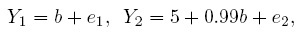
and e1 and e2 are measurement errors inherent in the two instruments. Assume also that σe1 = 0.01 grams and σe2 = 1 gram. This model is of the form (1.6).
Obviously these instruments have quite different characteristics and hence are not parallel. In fact, instrument 1 is much superior to instrument 2. In particular, it is correctly calibrated because its error-free measurement is identical to the true value, but this is not the case for instrument 2. There are two errors in the calibration of instrument 2—it has a fixed positive bias of 5 grams and a negative proportional bias of 1%. Instrument 1 has no bias of either kind and hence is accurate. These instruments have different measurement scales because what one measures as b is measured as 0.99b by the other. Note that the measurement scales are different despite the fact that the instruments have the same unit of measurement (grams). The scales would have been the same if either the b in the expression for Y1 were 0.99b or the 0.99b in the expression for Y2 were b. Furthermore, instrument 1 is much more precise than instrument 2. The measures of similarity, defined in Section 1.7.1, have the following values:

Clearly, these instruments do not have perfect agreement. There are four factors that contribute to disagreement—different fixed biases (zero versus 5), different scales (b versus 0.99 b), different error variances (0.012 versus 1), and nonzero measurement errors (positive error variances for both). Notwithstanding the fact that the instrument 1 is much superior to instrument 2, they may be considered to have sufficient agreement for interchangeable use in a home as kitchen scales. It, however, seems unlikely that they can be used interchangeably, for example, in a jewelry store. Thus, the same degree of agreement may be sufficient for one purpose but not for another.
Suppose now that instrument 1 is also miscalibrated in the same way as instrument 2. In this case, the instruments may have sufficient agreement—but they agree on the wrong thing. In fact, we are able to identify a method as miscalibrated just because we assumed that the true weight of b grams is measured. In practice, however, we may not be able to say whether a method is miscalibrated because we generally do not have access to true values in method comparison studies.
This example can also be used to demonstrate the effect of between-subject variation on correlation. For example, if σb = 1, the correlation between Y1 and Y2 from (1.9) is 0.70, whereas if σb = 4, the correlation increases to 0.97.
1.9 CONTROVERSIES AND OUR VIEW
The analysis of method comparison studies has generated controversies in the medical and clinical chemistry literature. The core questions include what really should be the goal of a method comparison study and how should the method comparison data be analyzed. Generally, only one of the two goals is put forward, albeit not always explicitly: (1) evaluation of agreement between the methods with the rationale that they can be used interchangeably if they agree well; and (2) evaluation of similarity by comparing characteristics such as biases, precisions, and scales of the methods to learn how the methods differ. In the first case, the data analysis typically consists of inference on agreement measures, whereas in the second, it consists of inference on measures of similarity such as the bias difference and precision ratio.
Some authors who believe in the goal of agreement evaluation forcefully reject the notion of correlation and correlation-type measures of agreement as irrelevant because they strongly depend on the between-subject variation of the population (Sections 1.6 and 1.8 and Chapter 2). It is argued that if correlation-type measures are used, then a high degree of agreement can simply be achieved by collecting data over a wide range of measurement. This is because a wide range effectively ensures large between-subject variation, which in turn leads to large values for the correlation-type measures. As an alternative, measures based on differences in measurements are suggested. In most cases, the popular approaches to inference on agreement measures do not emphasize explicit modeling of data, which is often considered unnecessary or too complicated to explain to practitioners who may be non-statisticians.
On the other hand, the authors who advocate comparing characteristics of methods criticize the goal of agreement evaluation as being too restrictive and often reject inference on agreement measures as serving a limited purpose. It is often asked: “What if the methods do not agree well?” Without comparing accuracies, precisions, and scales of the methods, we would not know why the methods disagree. Perhaps they disagree because one method is much better (e.g., much more precise) than the other or because they have different scales of measurement. But this analysis requires appropriate modeling of data, which often involves the correlation.
This book takes the view that both the aforementioned goals—evaluation of similarity and agreement—ought to be accomplished in the same method comparison study because the goals are interrelated and complementary (Sections 1.4 and 1.7.2). The key to accomplishing both goals is collecting data using sufficiently informative designs and appropriate modeling of data. There is universal agreement that the paired measurements design—which unfortunately is the most common design in practice—is completely inadequate for method comparison studies. The data from this design do not allow identifiability of the basic model parameters. Moreover, these data often do not even have sufficient information to reliably estimate precisions of the methods, making the comparison of precisions an unattainable goal (Section 1.12). At the very least, two measurements are needed from each method on every subject under identical conditions.
While the correlation-type agreement measures may mask important differences in the methods, there are other measures of agreement that do not have this drawback (see Chapter 2). We recommend examining more than one agreement measure because different measures quantify disagreement by looking at different aspects of the bivariate distribution of measurements from the two methods.
In this book, we espouse a model-based approach for the analysis of method comparison data. First, we fit an appropriate model to the data. Then, we use the fitted model to perform statistical inference on measures of similarity and agreement using standard tools of inference such as confidence intervals. This approach is illustrated in subsequent chapters of the book under various settings.
1.10 CONCEPTS RELATED TO AGREEMENT
The terms repeatability, reliability, and reproducibility are often used in the context of agreement evaluation. Repeatability of a measurement method refers to the variability in its repeated measurements made on the same subject under identical conditions. In this case, the true underlying value does not change, nor does the accuracy and precision of the method. Hence any variation in the repeated measurements is purely due to the inherent error in the measurement process. Thus, repeatability of a method refers to the size of its measurement errors. This explains why the error standard deviation is often called the repeatability standard deviation (Section 1.3.1). One can also think of this standard deviation as a measure of intra-method agreement.
Reliability, defined in (1.4), is also a characteristic of a measurement method that depends on the size of its measurement errors, but this size is measured relative to subject-to-subject variation in the true measurements.
Reproducibility is not a characteristic of a measurement method. It refers to the variation in the measurements made on the same subject under changing conditions. The “changing conditions” may be different instruments, different laboratories, or more generally, different measurement methods. The true value of the subject and the accuracy and precision of the measurement method may change between the conditions. If, however, the interest is in a small number of fixed and specified conditions, that is, the “condition” can be considered a fixed effect as opposed to a random effect, and the true value does not change between the conditions, then reproducibility is simply a synonym for agreement.
Equivalence is often used as a synonym for agreement, but it has a precise meaning in the statistical literature that differs from the notion of agreement. The concept of equivalence arises in the context of hypothesis testing. Equivalence hypothesis is used when the goal of the study is to demonstrate practical equivalence rather than a significant difference. For example, suppose φ is a scalar parameter of interest. In a typical significance testing problem, the null ( H0) and alternative ( H1) hypotheses are of the form
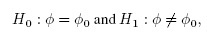
where φ0 is a specified reference value. In contrast, in an equivalence testing problem, the corresponding hypotheses are of the form

where (φ0 − ε1,φ0 + ε2) is a specified “indifference zone” that consists of values of φ that are practically the same as φ0. Equivalence testing is applied extensively in bioequivalence trials.
1.11 ROLE OF CONFIDENCE INTERVALS AND HYPOTHESES TESTING
1.11.1 Formulating the Agreement Hypotheses
Since agreement evaluation involves deducing whether two methods have sufficient agreement, it is natural to formulate this problem as a test of hypothesis. The question then becomes the following: Should the claim that “the methods have sufficient agreement” be formulated as the null hypothesis or the alternative hypothesis?
The answer to this question has important practical implications as statistical tests do not treat the null and alternative hypotheses in a symmetric manner. A test presumes that the null hypothesis is true and looks for evidence in the data against this hypothesis. If the data have strong evidence against the null, the test rejects the null in favor of the alternative; otherwise, the test accepts the null. Thus, the null hypothesis is treated like the default hypothesis—it is rejected only when the data strongly favor the alternative hypothesis.
A hypothesis test makes one of two types of errors. It makes a type I error if the test incorrectly rejects the null hypothesis (i.e., it incorrectly accepts the alternative hypothesis), and a type II error if it incorrectly accepts the null hypothesis. Ideally, we would like to have small probabilities for both the errors, but this is not possible for a test based on a fixed sample size. Therefore, a test is designed to ensure that its type I error probability is at most a prespecified small probability—also known as the level of significance. But the test has no control over its type II error probability, or its power, which is defined as 1 minus the probability of type II error. This is why the null and alternative hypotheses are formulated in a way that ensures that the more serious of the two errors becomes the type I error whose probability is guaranteed to be small. It is also expected that a power analysis is done prior to data collection and enough sample size is taken so that the test has adequate power to reject the null hypothesis when the alternative hypothesis is true.
The above arguments make it clear that whether “sufficient agreement” should be formulated as the null or the alternative hypothesis is determined by which of the two errors—the error of incorrectly declaring sufficient agreement or the error of incorrectly declaring insufficient agreement—is considered more serious. From the viewpoint of a user, clearly the former is the more serious error, and this should be the type I error. Therefore, the hypotheses for agreement evaluation should be formulated as
H1 : The two methods have sufficient agreement.
We refer to these hypotheses as the agreement hypotheses.
Suppose now that φ is a scalar measure of agreement. As mentioned in Section 1.5, this φ is a given function of parameters of the bivariate distribution of (Y1, Y2) (see also Chapter 2). In some cases, a large value for φ implies good agreement, whereas in some other cases, a small value implies good agreement. Let φ0 be the threshold for sufficient agreement specified by the practitioner. This threshold represents the value of φ beyond which the agreement is considered acceptable. When a small φ means good agreement, (1.13) becomes
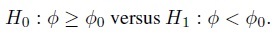 (1.14)
Alternatively, when a large φ means good agreement, (1.13) becomes
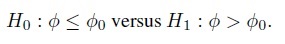 (1.15)
In either case, the agreement hypotheses are one-sided and require the threshold φ0. Statistical considerations alone cannot determine this threshold, or more generally, allow one to assess whether a given value of φ represents sufficient agreement. This is because a φ0 that is sufficient for one application may not be so for another.
1.11.2 Testing Hypotheses Using Confidence Bounds
Although the agreement hypotheses can be tested directly, we prefer the use of the corresponding one-sided confidence bound for φ. This is because a confidence bound provides additional information about the magnitude of φ besides being useful for testing hypotheses.
In particular, when a small value for φ implies good agreement, we can compute a 100(1 − α)% upper confidence bound for φ, say U. This U can be interpreted as the largest plausible value of φ supported by the data and it represents the least plausible amount of agreement as suggested by the data. Further, U can be used for testing the agreement hypotheses at significance level α in the following way:
This decision rule corresponds to the formulation in (1.14) (Exercise 1.4).
Similarly, when a large value for φ implies good agreement, we can compute a 100(1 − α)% lower confidence bound for φ, say L. This L leads to the following decision rule:
and provides a level α test of the hypotheses in (1.15).
1.11.3 Evaluation of Agreement Using Confidence Bounds
The use of confidence bounds offers an important practical advantage over hypothesis tests. The test requires an advance specification of the threshold φ0 for acceptable agreement, which may be a difficult task for the practitioner. On the other hand, the confidence bounds L or U can be computed without having to specify a φ0. They can be directly used to evaluate agreement by assessing whether the magnitude of agreement that the bound represents can be considered sufficient. If the answer is yes, infer sufficient agreement; otherwise infer insufficient agreement. This way the agreement can be evaluated without resorting to an explicit test of hypothesis.
In agreement evaluation, sometimes one wonders whether to compute a one-sided confidence bound for the agreement measure φ or a two-sided confidence interval for it. The choice is guided by the use to which the result will be put. If the result will be used to infer whether the methods have sufficient agreement, which is generally the case, then an appropriate one-sided bound is the more relevant choice. This bound can be used either directly to infer sufficient agreement or it can be used to explicitly test the agreement hypotheses (1.13). If, however, the result will be used to examine the plausible values of φ supported by the data, then a two-sided interval is the more relevant choice.
It may be noted that a two-sided 100(1 − α)% confidence interval for φ can also be used to provide a level α test of the one-sided agreement hypotheses. But this test will be less powerful than the one based on the relevant one-sided bound (Exercise 1.4). We use confidence bounds for agreement measures throughout the book.
1.11.4 Evaluation of Similarity Using Confidence Intervals
Since the evaluation of similarity involves deducing whether two methods have similar characteristics, it is appropriate to consider the equivalence testing methodology described in Section 1.10. In particular, one can specify an indifference zone around each measure of similarity defined in Section 1.7.1 and test the resulting hypothesis of equivalence. The indifference zones, for example, may be taken as

which essentially means that up to 5 units difference in fixed biases and up to 20% difference in measurement scales (or precisions or sensitivities) are acceptable.
We, nevertheless, eschew formal equivalence testing in this book in favor of two-sided confidence intervals for the similarity measures. This is because there is more than one measure of similarity and an indifference zone around each may lead to a substantial lack of overall agreement. We prefer to let the net effect of the differences in characteristics of methods be reflected in the values of agreement measures. These values can then be evaluated to see whether the extent of agreement may be considered sufficient. Besides, the confidence intervals of the similarity measures do reveal how much they differ from their ideal values. They can also be used to test equivalence hypothesis if needed.
1.12 COMMON MODELS FOR PAIRED MEASUREMENTS DATA
The paired measurements design is the most common design used for comparing two methods. It involves taking one measurement from each method on every subject in the study. Suppose there are n subjects. Let Yij denote the observed measurement from the j th method on the i th subject, i = 1, ..., n, j = 1, 2. For the purpose of modeling the data, we assume that the subjects are randomly selected from the population of interest, and treat the paired measurements (Yi1, Yi2) to be independently and identically distributed (i.i.d.) as (Y1, Y2). It follows that the measurement differences Di = Yi2 − Yi1 are i.i.d. as D = Y2 − Y1.
Often in practice, the subjects are selected deliberately rather than randomly so as to make the measurement range as wide as possible. The deliberate selection is reasonable from the viewpoint of experimenters as they would naturally like to compare the methods over the entire measurement range. But a model that takes such deliberate selection into account involves additional complications and is beyond the scope of this book.
Let Ȳ·j and Sj2, respectively, denote the mean and variance of the sample from the j th method. Further, let S12 and R, respectively, denote the sample covariance and sample correlation between the paired measurements. These statistics are defined as
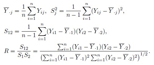 (1.16)
It is assumed that S1,S2 > 0, and | R | < 1. Let
 (1.17)
denote the sample mean and sample variance of the differences. Clearly, ![]() and
and ![]() Except for the sample correlation R, all the above statistics are unbiased estimators of their population counterparts.
Except for the sample correlation R, all the above statistics are unbiased estimators of their population counterparts.
We now present three commonly used models for the paired measurements data. The first two are related to the measurement error model (1.6) introduced in Section 1.6, and the last is a simple bivariate normal model. All assume normality.
1.12.1 A Measurement Error Model
This model assumes that (Y1, Y2) follows the measurement error model presented in (1.6), which allows for potentially different measurement scales for the methods. Hence the model for the paired measurements ( Yi1, Yi2) can be written as
 (1.18)
where bi is the true unobservable measurement for the ith subject and eij is the random error of the j th method (j = 1,2). Further, bi and eij are i.i.d. as b and ej, respectively, where b and ej are as defined in (1.6). In addition to the assumptions listed in Section 1.6, we assume that b and ej are normally distributed, that is, b ∼N1(µb, σ2) and ej ∼N1(0, σ2b).
This model implies that the pairs (Yi1, Yi2) are i.i.d. as (Y1, Y2), which follows a bivariate normal distribution with mean vector given by (1.7) and covariance matrix given by (1.8). The measurement differences Di and D can be written as

They depend on the true measurement as well as the differences in fixed biases and the measurement errors. In particular, the Di increase or decrease in proportion to the true values. This phenomenon is simply a consequence of unequal measurement scales. The Di are i.i.d. as D ∼N1(ξ, τ2), where ξ and τ2 are given in (1.10).
Under the model (1.18), all four measures of similarity described in Section 1.7.1, viz., β0, β1, λ, and γ2, can be used to compare characteristics of the methods.
Unfortunately, this measurement error model is not identifiable and hence its parameters cannot be estimated. The problem here is that there are six unrelated parameters in the model but we have only five sufficient statistics, namely, two sample means, two sample variances, and one sample covariance, under the bivariate normality of the data.
This problem of model non-identifiability can be resolved by making an assumption about one of the parameters, reducing the number of unknown parameters to five. Then, these parameters can be estimated using the maximum likelihood (ML) method. One possibility is to assume β1 = 1, that is, the methods have the same scale. In this case, the model reduces to the mixed-effects model described in the next section. Another possibility is to assume that the precision ratio λ is known, that is, the precision of one method is a known multiple of the precision of the other. Under this assumption, the fitting of the model is known as Deming regression (see Section 1.14.2).
1.12.2 A Mixed-Effects Model
This is a special case of the measurement error model (1.18) obtained by taking β1 = 1, thereby assuming that the two methods have the same measurement scale. Thus, we obtain
 (1.19)
Interpretations of the terms in the model and assumptions regarding them are identical to those stated for the model (1.18).
This model is popularly known as the Grubbs model. It is a variance components model with three components of variance, namely, σb2, σe21, and σ2e2. It can also be called a mixed-effects model because β0 is a fixed effect and bi is a subject-specific random effect. We can write this model in the familiar mixed-effects model form by assuming, without any loss of generality, that E( b)=0 and writing Yij = µj + bi + eij, where µ1 = µb and µ2 = β0 + µb. This is also the form we use in the subsequent chapters of the book.
The model (1.19) implies that the measurement pairs (Yi1, Yi2) are i.i.d. as (Y1, Y2), which follows a bivariate normal distribution with mean vector
 (1.20)
and covariance matrix
 (1.21)
Further, the correlation between the methods is
 (1.22)
These expressions can also be obtained by setting β1 =1 in (1.7), (1.8), and (1.9). The correlation here is non-negative, and as noted in Section 1.6.2, warrants a careful interpretation because it depends on the between-subject variation.
The measurement differences Di and D can be written as
 (1.23)
They are just a sum of differences in the systematic biases of the methods and their measurement errors, and are free of the true measurement bi. This contrasts with the case of measurement error model (1.18) where the differences depend on bi. The Di are i.i.d. as D ∼N1(ξ, τ2), where
 (1.24)
Since the measurement methods following the mixed-effects model have the same scale, their error-free measurements differ only by a constant (b versus β0 + b). As a result, the methods are assumed to be essentially tau equivalent (see Table 1.1). In other words, the methods may differ only on two characteristics—fixed bias and precision, and these differences can be measured by the similarity measures β0 and λ (Section 1.7.1). Unlike the case of measurement error model (1.6), the measure β0 for this mixed-effects model is actually the mean difference ξ.
The mixed-effects model (1.19) can be fit by the ML method. Any statistical software capable of fitting such models can provide the parameter estimates and their estimated covariance matrix. These estimates are used to perform inference on measures of agreement and similarity (see Chapter 2). Exercise 1.5 explores a simple method of moments approach for fitting this model. This method, however, may lead to negative estimates of error variances (see Exercise 1.6 for a real example). Besides, when the assumed model holds, the ML method is generally a more efficient method of estimation than the method of moments. Moreover, the latter does not generalize well for fitting more complicated models. For these reasons, we do not emphasize the method of moments in this book.
Although it is possible to get ML estimates of the error variances σ2ej from the paired measurements, the estimates may be unreliable as they may have unrealistically large standard errors. In practice, it often happens that one estimate is zero (the smallest possible value for the variance) or near zero and the other is larger by several orders of magnitude (see Exercise 1.6). This gives the false impression that one method has near-perfect precision whereas the other is substantially worse. If we rule out the possibility that the precisions of the methods may truly differ by several orders of magnitude, then this phenomenon usually indicates one of two possibilities: either (1) an entirely wrong model is being fit to the data (e.g., the assumption of equal scales is incorrect), or (2) the model is reasonable, but the data do not have enough information to reliably estimate the error variances.
Often in practice, the mixed-effects models are fit by the method of restricted maximum likelihood (REML) instead of the ML method. Although a discussion of the REML method is outside the scope of this book (see Bibliographic Note), here we just note that this method, by design, only estimates the variance-covariance parameters and not the fixed-effect parameters. Since this method does not jointly estimate all model parameters, it does not provide a joint covariance matrix of all parameter estimates. This matrix, however, is needed for inference on agreement measures because they are functions of both fixed-effect and variance-covariance parameters. Therefore, we do not use the REML method in this book.
A limitation of the mixed-effects model is its assumption of a common scale of measurement for both methods. The methods may have different scales despite having the same nominal unit of measurement.
1.12.3 A Bivariate Normal Model
This model simply assumes that (Y1, Y2) follows a bivariate normal distribution with mean (µ1,µ2), variance (σ12, σ22), and covariance σ12 (or correlation ρ ), and the paired measurements (Yi1, Yi2) form an i.i.d. sample of size n. Thus, the differences Di are an i.i.d. sample from the distribution of D ∼N1(ξ, τ 2).
The paired measurements in the previous two models also follow a bivariate normal distribution. But these models make specific assumptions about how the observed measurements are related to the true measurements and the measurement errors. These assumptions induce some structure in the means and the variance-covariance parameters of the bivariate normal distribution that may be seen by examining the expressions for these parameters in (1.7), (1.8), (1.20), and (1.21).
In contrast, the bivariate model in this section does not make any such assumptions on its parameters. As a result, while the model is identifiable, unlike the previous two models, it does not allow inference on any measure of similarity. Of course, one can compare the means and variances of the methods by examining the mean difference µ2 − µ1 and variance ratio σ22 /σ12. In fact, when the mean difference is close to zero and the variance ratio is close to one, we can validly conclude that the methods have similar characteristics. But we saw in Section 1.6.2 that the effects of difference in fixed biases and scale differences get confounded in µ2 − µ1, and the effects of scale differences and unequal precisions get confounded in σ22/σ12. Therefore, when the mean difference and the variance ratio are quite far from their respective ideal values of zero and one, we cannot be sure what the cause is in terms of the parameters of our interest. For example, it may be a difference in bias, scale, precision, or a combination thereof. Moreover, the variances σ12 and σ22 may be dominated by the between-subject variation. In such a case, the effect of unequal precisions may be missed by the variance ratio.
The bivariate normal model has five parameters—µ1, µ2, σ12, σ22, and ρ. Their ML estimators are simply their sample counterparts given in (1.16) with n −1 in the denominator replaced by n. The same is true for the ML estimators of ξ and τ2, which are functions of the model parameters.
Which of the three models should be used? This is mostly a rhetorical question if paired measurements data are all we have. One would like to fit the measurement error model (1.18) as it offers the most flexibility, but this model is not identifiable without additional assumptions. The next best option is to fit the mixed-effects model (1.19), but often the error variances cannot be estimated in a reliable manner. This often makes the bivariate normal model the only viable option. This model makes the fewest assumptions but is also the least informative among the three models for our purposes.
1.12.4 Limitations of the Paired Measurements Design
The paired measurements design is wholly inadequate for method comparison studies because the resulting data do not have sufficient information to allow estimation of all model parameters of interest. In particular, the measurement error model (1.18) is not identifiable on the basis of paired measurements alone, unless one is willing to make a potentially restrictive assumption (e.g., identical measurement scales or known precision ratio). Thus, the assumption that needs to be made a priori is unfortunately one of the issues that must be investigated in a method comparison study. To make matters worse, even if the model (1.19) with common measurement scale is assumed, we have seen in Section 1.12.2 that the data may not have enough information to reliably estimate such key parameters as the precisions of the methods. These serious difficulties show that the data need to be collected using designs that are more informative than the paired measurements design. A particularly attractive option is to use a repeated measurements design, where the measurements are replicated from each method on every subject. Modeling and analysis of such repeated measurements data are discussed in Chapter 5.
1.13 THE BLAND-ALTMAN PLOT
Consider the paired measurements data (Yi1, Yi2), i = 1,...,n. Their differences are Di = Yi2 − Yi1 and let their averages be Ai =(Yi1 + Yi2) /2. The Bland-Altman plot is a plot of the difference Di on the vertical axis against the average Ai on the horizontal axis. Although the limits of agreement are superimposed on this plot, we defer their discussion to the next chapter. The average Ai serves as a proxy for the true unobservable measurement bi. This plot is an invaluable supplement to the usual scatterplot of the paired measurements. There is much empty space in a typical scatterplot as the points tend to tightly cluster around a line, making it hard to see any patterns that may be present. But the plot of difference against average magnifies key features of disagreement such as fixed and proportional biases, and also helps in diagnosing common departures from assumptions regarding data such as the presence of outliers and heteroscedasticity.
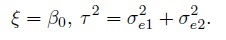
As an illustration, Figure 1.2 shows scatterplots and Bland-Altman plots for two simulated datasets, each with n = 100. The first dataset is simulated from the measurement error model (1.18) with the following parameter values:

In this case, the methods have a 15% difference in proportional biases. Although the scatterplot of these data in panel (a) shows a systematic difference in the methods, it may be hard to see that the difference is in proportional biases and not in fixed biases. However, as explained in Section 1.13.2 below, the linear trend in the Bland-Altman plot in panel (b) does suggest that the difference may be in proportional biases.
The second dataset is simulated from the mixed-effects model (1.19) with the following parameter values:

In this case, the precision ratio λ, given by (1.11), is 1/9, meaning that method 1 is nine times more precise than method 2. But this difference is difficult to discern in the scatterplot in panel (c), whereas the upward linear trend in the Bland-Altman plot in panel (d) indicates this possibility, see Section 1.13.2.
1.13.1 The Ideal Plot
The ideal Bland-Altman plot results in the case when the mixed-effects model (1.19) holds and the two methods have equal fixed biases and error variances. To see how this plot should look, note that if the model (1.19) holds, then from (1.23), the distribution of differences does not depend on the true values. Next, if the fixed biases are equal, then from (1.24), the differences have mean zero. Further, if the error variances are equal, then from Exercise 1.7, the differences are uncorrelated with the averages. It, therefore, follows that the points in the ideal Bland-Altman plot are scattered around zero in a random manner. Such a plot resembles the ideal plot of residuals versus fitted values in a regression analysis. If the points in the plot are not centered at zero, this suggests a difference in the fixed biases of the methods. Moreover, any pattern in this plot, such as a trend, nonconstant spread, or presence of outliers may suggest a potential failure of the model (1.19).
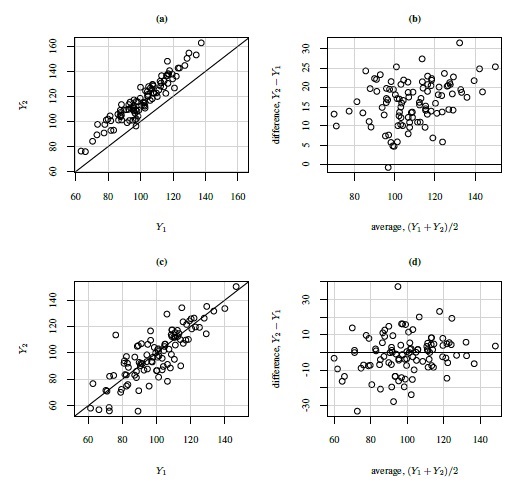
Figure 1.2 Scatterplots (panels (a) and (c)) and Bland-Altman plots (panels (b) and (d)) for two simulated datasets. The line of equality and the zero line are, respectively, superimposed on the two plots.
For a real example of the ideal situation, consider the oxygen saturation data. In this dataset, percent saturation of hemoglobin with oxygen is measured in 72 adult patients receiving general anesthesia or intensive care with two instruments. One is an oxygen saturation monitor (OSM) that uses arterial blood to take measurements, and the other is a pulse oximetry screener (POS) that is noninvasive and easy to use. Figure 1.3 displays these data. The Bland-Altman plot represents an ideal situation as the points are centered at zero and do not exhibit any pattern. Thus, we may conclude that the methods have similar fixed and proportional biases, and equal variances. The latter implies equal error variances for the methods unless they are dominated by the between-subject variation (see the next section). The scatterplot too does not show any evidence of unequal biases. Hence there is indication that the model (1.19) holds well. We return to these data in Chapter 4.
Figure 1.3 Plots for oxygen saturation data. Panel (a): Scatterplot with line of equality. Panel (b): Bland-Altman plot with zero line.
1.13.2 A Linear Trend in the Bland-Altman Plot
A departure from the assumptions behind the ideal Bland-Altman plot results in patterns in the plot. Two frequently seen patterns are a linear trend and heteroscedasticity. A linear trend indicates a correlation between differences and averages. A formal test for this trend is discussed later in Section 1.15.3. Since the averages serve as a proxy for the true measurements, this trend may suggest a relation between differences and true values. But from (1.23), such a relation is a violation of the equal proportional biases (or scales) assumption of the mixed-effects model (1.19). Nevertheless, it may also be that this model holds well for the data and the trend simply indicates a difference in precisions of the methods. These phenomena can be seen in Figure 1.2 where both Bland-Altman plots exhibit a trend. But the cause of the trend in panel (b) is unequal proportional biases, whereas it is unequal precisions in panel (d).
To understand the causes behind the trend, consider the measurement error model (1.18). Under this model, we have (Exercise 1.7)
This covariance is nonzero when the Bland-Altman plot exhibits a linear trend. It is zero when β1 = 1 and σe12 = σe22 and when the covariance is nonzero, at least one of these two conditions fails to hold. Thus, in explaining a linear trend, the effect of unequal proportional, biases (i.e., β1 ≠ 1) gets confounded with the effect of unequal precisions (i.e., σe12 ≠ σe22). Hence, on the basis of the plot alone, we cannot be sure whether the presence of a trend is due to unequal proportional biases, meaning that the mixed-effects model does not hold; or whether this model holds but the methods have unequal precisions. That said, if a trend is seen, it is most likely due to unequal proportional biases because the between-subject variance σb2 dominates the error variances. Therefore, we generally take the lack of a trend to imply equal proportional biases. It is also a good idea to use this plot together with the scatterplot of data, which may confirm the presence of a systematic difference between the methods (see, e.g., Figure 1.2, panel (a)).
One way to deal with the linear trend in the Bland-Altman plot is to remove it by a suitable transformation of measurements. The (natural) log transformation is often successful for this purpose. This transformation has the additional advantage that differences of log-scale measurements can be interpreted as logs of ratios of original measurements. No other transformation is generally suggested because the differences on transformed scale are difficult to interpret in terms of original measurements. If the log transformation fails or a curvilinear trend is seen in the plot, explicit modeling of the trend using a regression model may be called for.
As an illustrative example, consider the plasma volume data displayed in Figure 1.4. These data consist of measurements of plasma volume expressed as a percentage of normal in 99 subjects, using two sets of normal values—one due to Nadler and the other due to Hurley. The Bland-Altman plot in panel (b) clearly shows a linear trend, and the point cloud in the scatterplot in panel (a) is not parallel to the line of equality, confirming that the methods have unequal proportional biases. It is also clear from the plot in panel (c) that the log transformation is successful in removing the trend. But this plot is not centered at zero, meaning that after the transformation, there is a difference in the fixed biases of the methods. The scatterplot in panel (c) essentially confirms this observation. The impact of log transformation is highly visible in the Bland-Altman plots whereas it is less noticeable in the scatterplots. We return to these data in Chapter 4.
1.13.3 Heteroscedasticity in the Bland-Altman Plot
Heteroscedasticity refers to a change in the vertical scatter of the plot as the average increases. It indicates that the variability of the difference changes with the magnitude of measurement. This pattern is generally caused by dependence of the error variation of one or both methods on the magnitude of measurement. One of the most common patterns of heteroscedasticity is a fan shape, which typically occurs when the error variation increases in a constant proportion to the magnitude of measurement. Often, a log transformation of data removes this kind of heteroscedasticity. Potentially other transformations may stabilize the variance as well. But they are generally not used because of the difficulty in interpreting the transformed scale differences. If the log transformation does not succeed or the plot exhibits a complex pattern of heteroscedasticity, modeling of the variation may be necessary (see Chapter 6).
Figure 1.5 shows scatterplots and Bland-Altman plots of vitamin D data. This dataset consists of vitamin D concentrations (ng/mL) in 34 samples measured using two assays. There are two noteworthy features of these data. First, the Bland-Altman plot in panel (b) shows a fan-shaped heteroscedasticity, which is impossible to see in the scatterplot in panel (a). Further, as panel (d) shows, the log transformation of the data successfully removes this heteroscedasticity. Second, there are three outliers in the data, with values that are much larger than the rest. But these outliers play a special role as they allow the comparison of assays over the range of 0–250, whereas without them, the assays may only be compared over the range of 0–50. Notice also an additional outlier in the top left corner of panel (d), which is difficult to see in other plots. This outlier may be the result of an error in conducting the experiment or in recording of data, or it may be a bona fide value. Regardless of its origin, this outlier is likely to exert considerable influence on results due its location in the point cloud. Hence it is necessary to assess its impact on overall conclusions by doing the analysis with and without it. We consider this in Chapter 4.
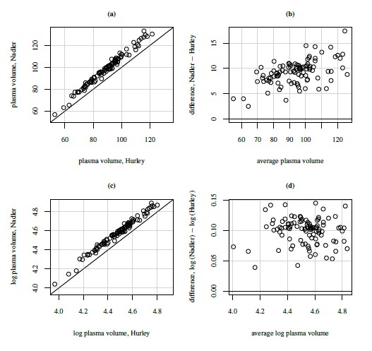
Figure 1.4 Scatterplots and Bland-Altman plots for plasma volume data. Panels (a) and (b) show measurements on original scale (%); panels (c) and (d) show log-scale measurements. The line of equality and the zero line are, respectively, superimposed on the two plots.
1.13.4 Variations of the Bland-Altman Plot
Three variations of the Bland-Altman plot are often considered in practice. The first one is suggested when one method in the comparison is a reference or gold standard. In this case, the measurements Yi1 from the reference method are plotted on the horizontal axis because the Yi1 are thought to be a better proxy for the true measurements than the average measurements. Assuming the measurement error model (1.18) for the data, it can be seen that
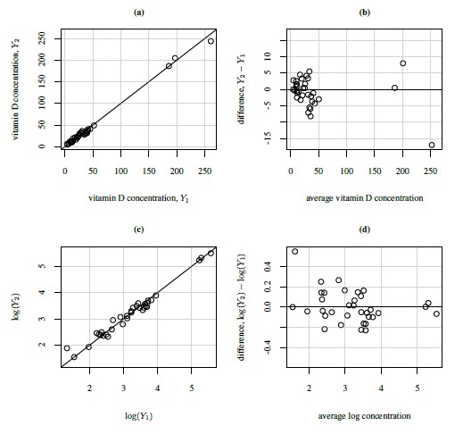
Figure 1.5 Scatterplots and Bland-Altman plots for vitamin D data. Panels (a) and (b) show measurements on original scale (ng/mL); panels (c) and (d) show log-scale measurements. The line of equality and the zero line are, respectively, superimposed on the two plots.
This covariance is zero if and only if β1 = 1 +(σe12/σb2). When β1 ≠ 1, it is highly unlikely that β1 precisely equals 1 + (σe12/σ2). On the other hand, when β1 = 1, this covariance is negative unless the reference method is error-free, in which case the covariance is zero. Combining the two cases, it is clear that the plot of differences against the reference measurements generally exhibits a trend, regardless of whether methods have equal proportional biases or not, unless, of course, the reference method is error-free. But since an error-free method is not available in method comparison studies, this plot is of limited use in detecting a difference in proportional biases of two methods. Nevertheless, it remains useful for diagnosing heteroscedasticity and detecting presence of outliers.
In the second variation, the Yi2 /Yi1 ratio is plotted on the vertical axis. In yet another variation, the difference between two methods expressed as a percentage of their average, that is, 100( Di /Ai)%, is plotted on the vertical axis. Just like the Bland-Altman plot, these are often better than the usual scatterplot at revealing key features of interest in a method comparison study. These alternatives are typically considered when the Bland-Altman plot shows either a trend or a nonconstant scatter.
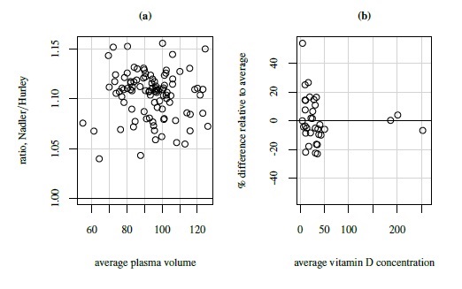
Figure 1.6 Variations of the usual Bland-Altman plot. Panel (a): Plot of ratio versus average for plasma volume data. Panel (b): Plot of relative difference versus average for vitamin D data. The horizontal lines in the plots, respectively, mark the points 1 and 0.
Sometimes when the differences are proportional to the true values, it may be that the ratios are free of the true values. So if the Bland-Altman plot has a trend, the ratio plot may not have it. This can be seen for plasma volume data in Figures 1.4 (panel (b)) and 1.6 (panel (a)). The ratio plot can also be used to get a rough estimate of β1 when β0 = 0, that is, the data in the usual scatterplot of Yi2 versus Yi1 are clustered around a line that has zero intercept. Further, if the Bland-Altman plot shows a fan-shaped pattern of heteroscedasticity implying that the variation in differences may be proportional to true values, the percent difference plot may show a constant scatter. This can be seen for vitamin D data by comparing panel (b) of Figures 1.5 and 1.6.
1.14 COMMON REGRESSION APPROACHES
1.14.1 Ordinary Linear Regression
The ordinary linear regression of a new method (Y2) on a reference method (Y1) is often suggested to study the relation between the two methods. Since Y2 is regressed on Y1, we say Y2 is a response variable and Y1 is an explanatory variable or a covariate. The ordinary linear regression presumes that the explanatory variable is error-free and only the response variable is measured with error. It posits that the paired measurements (Yi1, Yi2) follow the model
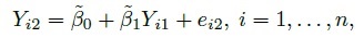 (1.25)
where the intercept ![]() and slope
and slope ![]() are fixed unknown coefficients; and ei2 is the random error of the new method. These errors are i.i.d. with mean zero and variance σe22, and are independent of reference method measurements. This model has the same form as the measurement error model (1.18) except for the important assumption that ei1 = 0, that is, there is no random error in the reference method. In other words, the observed Y1 is also the true measurement of the reference method. It may be noted that Y1 is still being treated as a random quantity rather than a fixed quantity, but Y1 inherits its variability solely from the variability in the true values. This contrasts with Y2, which has two sources of variability—the variability in the true value and the variability in the errors.
are fixed unknown coefficients; and ei2 is the random error of the new method. These errors are i.i.d. with mean zero and variance σe22, and are independent of reference method measurements. This model has the same form as the measurement error model (1.18) except for the important assumption that ei1 = 0, that is, there is no random error in the reference method. In other words, the observed Y1 is also the true measurement of the reference method. It may be noted that Y1 is still being treated as a random quantity rather than a fixed quantity, but Y1 inherits its variability solely from the variability in the true values. This contrasts with Y2, which has two sources of variability—the variability in the true value and the variability in the errors.
The model (1.25) can also be written as

This form makes it clear that the conditional mean of Y2 given Y1 is being modeled as a linear function of Y1. The function that describes the relation between E(Y2 | Y1) and Y1 is called the true regression function of Y2 on Y1. In ordinary linear regression, this function is linear and hence is referred to as the true regression line.
The regression coefficients ![]() and
and ![]() are commonly estimated using the method of least squares. The least squares estimators are those values of
are commonly estimated using the method of least squares. The least squares estimators are those values of ![]() and
and ![]() that minimize the sum of squares of errors in the response variable, which from (1.25) is
that minimize the sum of squares of errors in the response variable, which from (1.25) is
If the paired data are plotted in a scatterplot with response variable on the vertical axis and explanatory variable on the horizontal axis, the error ei2 represents the vertical distance of the point (Yi1, Yi2) from the true regression line. Therefore, the error sum of squares can be interpreted as the sum of squares of vertical distances between the observed data points and the regression line. Minimization of this sum of squares leads to the following least squares estimators (Exercise 1.11):
 (1.26)
where R, Ȳ·j, and Sj are given in (1.16). The estimators in (1.26) are unbiased for their population counterparts. The line ![]() is called the fitted regression line of Y2 on Y1. Here
is called the fitted regression line of Y2 on Y1. Here ![]() known as the predicted value or the fitted value of Y2, represents an unbiased estimator of the conditional mean E(Y2 | Y1).
known as the predicted value or the fitted value of Y2, represents an unbiased estimator of the conditional mean E(Y2 | Y1).
The assumptions underlying the ordinary regression model (1.25) need to be expanded in order to perform inference on the model parameters. It is common to assume that the data follow the bivariate normal model described in Section 1.12.3. The bivariate normality of (Y1, Y2) implies that the conditional distribution of Y2 | Y1 is normal with mean
which is a linear function of Y1. Thus, the linearity of the true regression function is not an additional assumption as it follows from the assumed bivariate normality. We can write this regression line in the form E(Y2 | Y1)= ![]() +
+ ![]() Y1 by taking
Y1 by taking
 (1.27)
Under the bivariate normal model, the least squares estimators of ![]() and
and ![]() in (1.26) are also their ML estimators (Exercise 1.11).
in (1.26) are also their ML estimators (Exercise 1.11).
The assumption of an error-free reference method in (1.25) is quite important. If it is violated, the least squares estimators in (1.26) do not estimate the intercept and slope of the true line around which the data are scattered. To see this, assume that the reference method also measures with error and the data follow the measurement error model (1.18). This model assumes that the data are scattered around a line with intercept β0 and slope β1. However, under this model, the regression line of Y2 on Y1 has coefficients ![]() and
and ![]() that can be obtained by substituting the expressions of moments from (1.7) and (1.8) in (1.27). This substitution yields
that can be obtained by substituting the expressions of moments from (1.7) and (1.8) in (1.27). This substitution yields
 (1.28)
Obviously, the coefficients (![]() ,
, ![]() ) of the regression line differ from the coefficients (β0, β1) of the true line unless σe12 = 0, implying an error-free reference method. In particular, | β˜1 | shrinks | β1 | by the factor σ2b/(σb2 + σe12), which represents the reliability (Section 1.6.2) of the reference method. This shrinkage phenomenon where the slope of the regression line is less than the true slope, in absolute value terms, is called the attenuation of slope caused by the error in the explanatory variable. The higher the reliability of the explanatory variable, the less severe is the attenuation. It also causes
) of the regression line differ from the coefficients (β0, β1) of the true line unless σe12 = 0, implying an error-free reference method. In particular, | β˜1 | shrinks | β1 | by the factor σ2b/(σb2 + σe12), which represents the reliability (Section 1.6.2) of the reference method. This shrinkage phenomenon where the slope of the regression line is less than the true slope, in absolute value terms, is called the attenuation of slope caused by the error in the explanatory variable. The higher the reliability of the explanatory variable, the less severe is the attenuation. It also causes ![]() to differ from β0 by the amount
to differ from β0 by the amount ![]() µb.
µb.
In summary, if the reference method is error-prone, the true regression line is not the line around which the data are scattered. In particular, if β1 and µb are both positive, the regression line tilts towards the horizontal axis resulting in reduced slope and increased intercept when compared to the true line. The difference between the two lines decreases as the reliability of the reference method increases, and the lines become identical when the reference is error-free. Note that there is nothing wrong per se with the least squares estimators (1.26), which correctly estimate the regression coefficients given by (1.28). It is just that these coefficients themselves do not represent the intercept and slope of the true line.
Figure 1.7 shows an example of difference between the two lines. It displays a scatterplot of n = 100 pairs of observations simulated from the model (1.18) with the following parameter values:

The data here are truly scattered around the line of equality. But, from (1.28), the true regression line of Y2 on Y1 has increased intercept ![]() = 22 and decreased slope
= 22 and decreased slope ![]() = 0.8. The least squares estimates of these coefficients, 22.9 and 0.77, are close to their respective true values.
= 0.8. The least squares estimates of these coefficients, 22.9 and 0.77, are close to their respective true values.
1.14.2 Deming Regression
Deming regression is a popular approach for fitting a line through the paired measurements (Yi1, Yi2), i = 1,...,n, when both the response variable Y2 and the explanatory variable Y1 are measured with error. This contrasts with ordinary regression where only the response variable is measured with error and the explanatory variable is error-free. In Deming regression, we assume that the data follow the measurement error model (1.18) and the ratio of error variances, λ = σe12/σe22, is known. The line ![]() is called the Deming regression line and also the orthogonal regression line. Here (
is called the Deming regression line and also the orthogonal regression line. Here (![]() ,
, ![]() ) is an estimate of (β0, β1) in the model (1.18) and
) is an estimate of (β0, β1) in the model (1.18) and ![]() is the value of Y2 predicted by the line when the other variable is Y1. Despite being called a regression line, this line does not estimate the true regression of Y2 on Y1, that is, E(Y2 | Y1)=
is the value of Y2 predicted by the line when the other variable is Y1. Despite being called a regression line, this line does not estimate the true regression of Y2 on Y1, that is, E(Y2 | Y1)= ![]() +
+ ![]() Y1, with coefficients given by (1.27).
Y1, with coefficients given by (1.27).
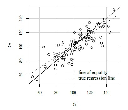
Figure 1.7 A scatterplot of simulated data superimposed with the line of equality, around which the data are truly scattered, and the true regression line of Y2 on Y1.
The coefficients in Deming regression are estimated using the method of orthogonal least squares. Assume for now that λ =1 so that the two variables are measured with equal precision. It is then natural to estimate the coefficients by minimizing the sum of squares of perpendicular (or orthogonal) distances of the points (Yi1, Yi2) from the line Y2 = β0 + β1 Y1. This is the method of orthogonal least squares. It is a generalization of the least squares method used in ordinary regression wherein the sum of squares of vertical distances is minimized because only the response variable, plotted on the vertical axis, is measured with error. Figure 1.8 displays the vertical and perpendicular distances from a point to a line. The latter is also the shortest distance between a point and a line.
The perpendicular from (Yi1, Yi2) intersects the line Y2 = β0 + β1 Y1 at the point (Yi1, Yi2), where

The perpendicular distance between the point (Yi1, Yi2) and the line Y2 = β0 + β1 Y1 equals the Euclidean distance between the points (Yi1, Yi2) and (![]() i1,
i1, ![]() i2) —see Figure 1.8. The square of this distance is
i2) —see Figure 1.8. The square of this distance is
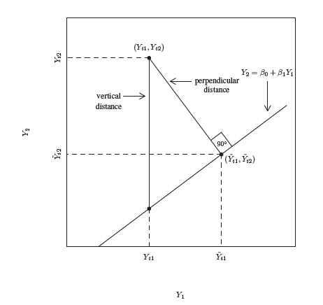
Figure 1.8 Vertical and perpendicular distances of a data point from a line. The former is used in ordinary least squares whereas the latter is used in orthogonal least squares.
which simplifies to
The orthogonal least squares estimators of coefficients in the Deming regression line are obtained by minimizing the sum of these squared perpendicular distances,
 (1.29)
with respect to (β0, β1). This sum is a weighted sum where the weight given to each data point is 1 /(1 + β12). Without the weights, this sum is simply the sum of squares of vertical distances, which is minimized in ordinary least squares.
Consider now the general case when λ may be any known value, not necessarily one. In this case, it is not appropriate to minimize the sum of squares of perpendicular distances because the two variables are not measured with equal precision. Therefore, orthogonal least squares is applied after rescaling one of the variables, say Y1, by dividing it with ![]() to make the two error variances equal. This method leads to the following estimates of coefficients in the Deming regression line (Exercise 1.12):
to make the two error variances equal. This method leads to the following estimates of coefficients in the Deming regression line (Exercise 1.12):
 (1.30)
where
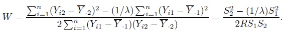
These estimators are also the ML estimators of (β0, β1) in model (1.18) with known λ.
It follows that Deming regression is equivalent to orthogonal regression only when λ = 1. If λ ≠ 1, Deming regression minimizes the sum of squared distances at an angle other than 90◦.
There is just one Deming regression line irrespective of whether Y1 or Y2 is used as the explanatory variable (Exercise 1.13). In other words, if ![]() is the Deming regression line for predicting Y2 from Y1, then the same line, written as
is the Deming regression line for predicting Y2 from Y1, then the same line, written as ![]() 1 = −(
1 = −(![]() 0 /
0 /![]() 1) + (1 /
1) + (1 /![]() 1) Y2, is the Deming regression line for predicting Y1 from Y2. This is intuitive as the perpendicular distance of a point from a line does not depend on the choice of explanatory and response variables. This contrasts with ordinary least squares where there are two different lines—one for the regression of Y2 on Y1, obtained by minimizing the sum of squares of vertical distances, and the other for the regression of Y1 on Y2, obtained by minimizing the sum of squares of horizontal distances. These two least squares lines are special cases of the Deming regression line, respectively, when one takes λ → 0, or Y1 is error-free, and when λ →∞, or Y2 is error-free (Exercise 1.14). It can also be seen that the Deming regression line falls between the two least squares lines. However, all three lines pass through the point (
1) Y2, is the Deming regression line for predicting Y1 from Y2. This is intuitive as the perpendicular distance of a point from a line does not depend on the choice of explanatory and response variables. This contrasts with ordinary least squares where there are two different lines—one for the regression of Y2 on Y1, obtained by minimizing the sum of squares of vertical distances, and the other for the regression of Y1 on Y2, obtained by minimizing the sum of squares of horizontal distances. These two least squares lines are special cases of the Deming regression line, respectively, when one takes λ → 0, or Y1 is error-free, and when λ →∞, or Y2 is error-free (Exercise 1.14). It can also be seen that the Deming regression line falls between the two least squares lines. However, all three lines pass through the point (![]() ·1,
·1, ![]() ·2). This phenomenon is illustrated in Figure 1.9 using the data displayed in Figure 1.7.
·2). This phenomenon is illustrated in Figure 1.9 using the data displayed in Figure 1.7.
1.15 INAPPROPRIATE USE OF COMMON TESTS IN METHOD COMPARISON STUDIES
We now describe some commonly used hypothesis tests that have limited value in method comparison studies. There is nothing wrong with these tests, but the resulting conclusions are not in line with the stated goals of the method comparison studies. All the tests discussed here are based on the paired measurements data and bivariate normality (Section 1.12.3) is assumed for them. Some tests additionally assume a measurement error model (Section 1.12.1) or a mixed-effects model (Section 1.12.2). We will also suggest appropriate modifications to these tests in order to address issues of direct concern in method comparison studies.
1.15.1 Test of Zero Correlation
To perform a test of significance for correlation ρ between Y1 and Y2 in a bivariate normal setup, one formulates the null and alternative hypotheses as
and computes the test statistic
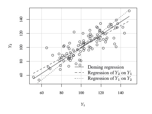
Figure 1.9 Deming regression line and the two ordinary least squares regression lines for the data displayed in Figure 1.7.
where R is the sample correlation defined in (1.16). This statistic follows a t distribution with n − 2 degrees of freedom when the null hypothesis is true. The test rejects the null hypothesis at level α if |T | > tn−2, 1−α/2.
Sometimes in practice a significant result of this test is taken as evidence of “agreement” between two methods. This, however, is clearly inadequate since correlation is a measure of linear relationship and not of agreement. Besides, two methods designed to measure the same quantity will rarely be uncorrelated. To determine the strength of correlation, a better alternative is to use a lower confidence bound for ρ. This bound indicates the worst case (i.e., the smallest) value of ρ that is plausible with the data. An approximate 100(1 − α)% lower bound for ρ is
 (1.31)
This formula works well when n is large. To understand how it is derived, consider the Fisher’s z-transformation of R, defined as
 (1.32)
which represents tanh−1(R). When n is large, z(R) approximately follows a normal distribution with mean z(ρ) and variance 1 /(n − 3). From this result, an approximate 100(1 − α)% lower confidence bound for z(ρ) is
The formula (1.31) now follows by transforming back this bound to the original scale by applying the inverse of the Fisher’s z -transformation.
1.15.2 Paired t-test
The paired t-test is a test of equality of means of the paired measurements (Y1, Y2). It is essentially the usual one-sample t-test of zero mean applied to the differences Di in the paired measurements. One sets up the null and alternative hypotheses as
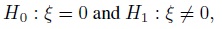
and computes ![]() , where
, where ![]() and SD are defined in (1.17). The test statistic T follows a t distribution with n − 1 degrees of freedom under H0. The level α paired t-test rejects the null hypothesis if |T | > tn−1, 1−α/2.
and SD are defined in (1.17). The test statistic T follows a t distribution with n − 1 degrees of freedom under H0. The level α paired t-test rejects the null hypothesis if |T | > tn−1, 1−α/2.
If in addition to bivariate normality, the data also follow the mixed-effects model (1.19), then from (1.24), ξ equals β0 the difference in fixed biases of the methods. Therefore, a test of ξ =0 is also a test of β0 = 0. This correspondence, however, fails to hold if the methods have unequal proportional biases. To see this, suppose now that the data follow the measurement error model (1.18). Then from (1.10), ξ = β0 +(β1 − 1) µb. As a result, testing for ξ =0 does not amount to testing for β0 = 0.
Being a test of equality of means, the paired t-test has limited value in method comparison studies (Section 1.11.4). If the null hypothesis of no difference in means is accepted, it may not be because ![]() is small (implying that its mean ξ may be small), but because S2D/n is large (implying that ξ is not estimated precisely either due to large variability in the differences or due to a small sample size). In other words, the test may simply have a low power. To examine the mean difference in paired measurements, a better alternative is to use a 100(1 − α)% confidence interval for ξ, given as
is small (implying that its mean ξ may be small), but because S2D/n is large (implying that ξ is not estimated precisely either due to large variability in the differences or due to a small sample size). In other words, the test may simply have a low power. To examine the mean difference in paired measurements, a better alternative is to use a 100(1 − α)% confidence interval for ξ, given as
where SD is the sample standard deviation of the paired differences. The interval gives the plausible values of ξ that are supported by the data.
1.15.3 Pitman-Morgan and Bradley-Blackwood Tests
The Pitman-Morgan test is a test for equality of variances of the paired measurements (Y1, Y2). It exploits a useful fact about the covariance between difference D and average A of the paired measurements. Since

the null hypothesis of equality of variances is equivalent to assuming zero correlation between D and A. Thus, to test
it actually tests the following hypotheses:

Since (Y1, Y2) and hence (D, A) follow a bivariate normal distribution, this null hypothesis can be tested by applying the test of zero correlation in Section 1.15.1 to (D, A) instead of (Y1, Y2). Thus, the test statistic is
where R1 is the sample correlation of the observed (D, A) values. The level α Pitman-Morgan test rejects the null hypothesis of equal variances if |T | > tn−2, 1−α/2.
If in addition to bivariate normality, the paired measurements also follow the mixed-effects model (1.19), then it can be seen that
This way the Pitman-Morgan test provides a test of equality of precisions of the methods. This test is also known as the Maloney-Rastogi test.
The Bradley-Blackwood test is a generalization of the Pitman-Morgan test as it simultaneously tests for equality of means and equality of variances of the paired measurements (Y1, Y2). Since (D, A) is bivariate normal, the conditional distribution of D given A is normal with mean

where

These ![]() and
and ![]() represent the intercept and slope of the linear regression of D on A. Moreover, since E(D)= µ2 − µ1 and cov(D, A)=(σ22 − σ12) /2, the hypothesis {µ1 = µ2,σ21 = σ22} is equivalent to {
represent the intercept and slope of the linear regression of D on A. Moreover, since E(D)= µ2 − µ1 and cov(D, A)=(σ22 − σ12) /2, the hypothesis {µ1 = µ2,σ21 = σ22} is equivalent to {![]() 0 =
0 = ![]() = 0}. Exploiting this equivalence, the Bradley-Blackwood test simultaneously tests the hypotheses
= 0}. Exploiting this equivalence, the Bradley-Blackwood test simultaneously tests the hypotheses

by actually testing the hypotheses

using an F-test of zero intercept and zero slope in the regression of D on A. From the standard linear regression analysis, this F-test is based on the statistic
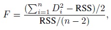
where RSS represents the residual sum of squares from the regression of D on A, and can be written as
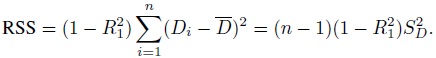
When the null hypothesis is true, the statistic follows an F distribution with numerator and denominator degrees of freedom 2 and n−2, respectively. The level α Bradley-Blackwood test rejects the simultaneous null hypothesis of equality of means and equality of variances when F>f2, n−2,1−α.
If the paired measurements actually follow the mixed-effects model (1.19), the Bradley-Blackwood test provides a simultaneous test of equality of fixed biases (β0 = 0) and equality of error variances (σe12 = σe22) of the two methods. Thus, it is a test of parallelism (Section 1.6.4) of the methods under the assumption of equal proportional biases for the methods.
Moreover, just like the paired t-test, these tests are also of limited value in method comparison studies because the hypotheses being tested are not the right ones (Section 1.11.4). To determine the extent of difference in variances of the paired measurements, one may use the following 100(1 − α)% confidence interval for σ22 /σ21 (Exercise 1.15):
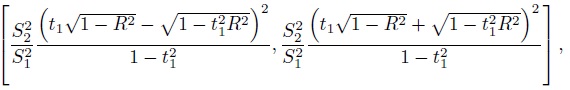 (1.33)
where ![]()
In a Bland-Altman plot (Section 1.13), we were interested in checking for a linear trend in D versus A. The null hypothesis of cor(D, A)=0 is equivalent to equality of variances of Y1 and Y2. Further, the simultaneous null hypothesis of (![]() ,
, ![]() ) = (0, 0) is equivalent to equality of means of Y1 and Y2 in addition to equality of their variances. Although these hypotheses may be tested using Pitman-Morgan and Bradley-Blackwood tests, we do not use them in the book as they test for significance, not for agreement.
) = (0, 0) is equivalent to equality of means of Y1 and Y2 in addition to equality of their variances. Although these hypotheses may be tested using Pitman-Morgan and Bradley-Blackwood tests, we do not use them in the book as they test for significance, not for agreement.
1.15.4 Test of Zero Intercept and Unit Slope
The test for zero intercept and unit slope is suggested in two contexts—the ordinary linear regression (Section 1.14.1) and Deming regression (Section 1.14.2) of Y2 on Y1. In either case, one generally sets up separate hypotheses for intercept and slope, namely,
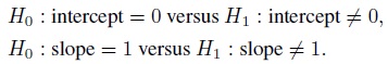
These hypotheses are tested individually.
In the case of ordinary regression, zero intercept and unit slope means E(Y2 | Y1)= Y1. Upon taking expectation on both sides with respect to Y1, we get µ2 = µ1—the equality of means of the methods. For the Deming regression, zero intercept and unit slope means tau-equivalence (Section 1.6.4) of the methods. In other words, the methods have equal fixed and proportional biases. Thus, in both cases, the sole concern is with differences in biases of the two methods. However, just like the other tests of equality in this section, these tests have rather limited usefulness as the null hypotheses may be accepted due to low power of the tests. Instead of testing for zero intercept and unit slope, a better alternative is to use confidence intervals for these parameters to examine their magnitudes.
Since the equality of means (or even tau-equivalence) of methods is not enough by itself for good agreement between them (Section 1.7.2), the testing for zero intercept and unit slope is often suggested only when the methods have high correlation. But this raises the question of how high the correlation should be before one can proceed to the regression step. Unfortunately, any answer to this question is likely to be arbitrary, especially since the correlation depends heavily on the range of the true values in the population.
The above discussion on the value of testing for zero intercept and unit slope tacitly assumes that the regression is fit appropriately. However, the ordinary regression is not appropriate for method comparison studies because it requires the explanatory variable Y1 to be error-free, which is generally not the case in practice. Further, the Deming regression requires the precision ratio λ to be known, which too is generally not the case. So λ is often replaced by an estimate based on error variances estimated from replicate measurements. But the use of an estimated λ as a known λ invalidates the use of original expressions for the standard errors of the estimates. Thus, the typical fitting of Deming regression in practice is also inappropriate. Moreover, if replications are available, it is more efficient to model all the data together and jointly estimate all the parameters to carry out inference on parametric functions of interest.
1.16 KEY STEPS IN THE ANALYSIS OF METHOD COMPARISON DATA
The key steps in the analysis of method comparison data are given below. These steps are illustrated throughout the book.
Perform exploratory analysis of data by displaying them graphically. Make both scatterplot and Bland-Altman plot. Superimpose the equality line in the scatterplot and the zero line in the Bland-Altman plot. Use the two plots in a complementary manner. Look for patterns in the plots. Look especially for evidence of outliers, fixed and proportional biases, and heteroscedasticity.
Other plots may also be useful such as the trellis plot. It is constructed as follows. The subjects are sorted in ascending order according to their average measurement. The vertical axis is divided into rows, one for each sorted subject, and each row displays all measurements for the corresponding subject. Different symbols are used for different methods. The vertical axis is labeled “sorted subject ID,” with ID = 1 referring to the subject with the smallest average, and so on. A key feature of this plot is that it shows within-subject variation. Figure 1.10 shows a trellis plot of log-scale plasma volume data. The Nadler measurements are higher than Hurley’s by an almost a constant amount. The data appear homoscedastic. The plots in Figure 1.4 led to the same conclusions.
- Model the data. Come up with a plausible model for the data. To the extent the model and the information in the data allow, let the model have method-specific parameters. Be sure to check goodness of fit and perform model diagnostics to verify the underlying assumptions.
- Evaluate similarity of methods by examining the confidence intervals for relevant measures of similarity. Use the fitted model to compute these confidence intervals.
- Evaluate agreement between the methods by examining confidence bounds for measures of agreement. Use a variety of agreement measures. Use the fitted model to compute the confidence bounds.
- Decide whether the methods agree sufficiently well to be used interchangeably. Identify causes of disagreement and see whether a simple recalibration of one of the methods may improve its agreement with the other. Be sure to check whether one method is clearly superior to the other.
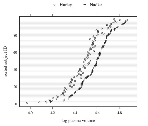
Figure 1.10 Trellis plot of log-scale plasma volume data. The subjects are sorted according to their average measurement.
1.17 CHAPTER SUMMARY
- A method comparison study has two complementary goals—evaluation of similarity and evaluation of agreement. The latter is the primary goal.
- Having similar characteristics is not enough for good agreement between methods.
- Finding an adequate model for data is a necessary step in the analysis of method comparison data.
- Agreement between methods is evaluated by performing model-based inference on measures of agreement. Generally, one-sided confidence bounds for agreement measures are more relevant for this purpose than their two-sided counterparts.
- Characteristics of methods are compared by performing model-based inference on measures of similarity. Generally, two-sided confidence intervals for similarity measures are appropriate for this purpose.
- The widely used paired measurement design is wholly inadequate for collecting data for method comparison studies. The measurements should be replicated by each method on every subject.
- Ordinary regression of a new method on a reference method is appropriate only when the reference method measures without error.
- Deming regression is appropriate only when the ratio of precisions of methods is known.
- Testing null hypothesis of equality should be avoided in favor of appropriate confidence intervals.
- In general, testing whether the regression line of one method on the other coincides with the 45◦ line does not amount to checking for good agreement.
1.18 BIBLIOGRAPHIC NOTE
Models for Measurements
The classical model (1.1) for measurements of a method is studied in detail in Fleiss (1986, Chapter 1) and Dunn (2004, Chapter 1). These authors, together with Barnhart et al. (2007a) and Bartlett and Frost (2008), provide a good discussion of the notions of accuracy, precision, repeatability, and reliability of a method.
Grubbs (1948) is one of the earliest articles devoted to comparison of methods. It essentially assumes the mixed-effects model (1.19) and estimates its parameters using the method of moments. The model (1.19) is also called the Grubbs model after this article. In the clinical chemistry literature, Westgard and Hunt (1973) use the measurement error model (1.18) for paired measurements. These authors call attention to pitfalls in interpretation of correlation coefficients and t-tests. But they also advocate the classical least squares regression as “potentially the most useful statistical technique” for analysis of method comparison data, provided a scatterplot of the data does not show nonlinearity and outliers. Cornbleet and Gochman (1979) point out that the classical least squares estimators of slope and intercept are incorrect if the independent variable is measured with error. To fit the model (1.18), they suggest the regression method of Deming (1943)—popularly known as Deming regression even though the method is originally due to Kummell (1879). See Finney (1996) for an interesting historical account of regression when both independent and dependent variables are measured with error.
Two assumptions in the model (1.18) are often violated in practice. The first is that the methods have uncorrelated measurement errors. Rifkin (1995) gives examples of clinical diagnostic methods with potentially correlated measurement errors and discusses the effect of this correlation on inference regarding the slope parameter. The second is that the error variances remain constant throughout the measurement range. Nix and Dunstan (1991) assume that the error variances are known, but they are free to vary from subject to subject in an unstructured manner. They propose an ML method to estimate the regression coefficients. The usual Deming regression is a special case of this method when the error variances do not change with subjects. Linnet (1990) lets the error standard deviations be proportional to the average of the true values of the subjects. He proposes an iteratively reweighted modification of Deming regression to estimate the regression coefficients. See Rubin (1983) for an introduction to the iteratively reweighted least squares technique. Martin (2000) describes an approach similar to Linnet (1990) but with different assumptions on error variances.
One may refer to the books by Searle et al. (1992), Vonesh and Chinchilli (1997), Pinheiro and Bates (2000), and Gelman and Hill (2007) for an introduction to mixed-effects models and their applications. These books also describe the ML and REML methods for fitting such models. The book by Cheng and Van Ness (1999) contains a comprehensive treatment of measurement error models. Kutner et al. (2004) provide a good introduction to linear regression models. A rigorous introduction to statistical inference is provided by Casella and Berger (2001). It also provides (in Chapters 11 and 12) a succinct account of the ordinary regression model and the measurement error model. Graybill (2001) is a handy reference on matrix algebra.
Deming Regression and Alternatives
Dunn (2007) notes that Deming regression has limited application in practice because it requires the error variance ratio to be known, which is generally not the case. It is common to deal with this issue by simply replacing the unknown ratio with the ratio of error variances estimated using replications from the present experiment or from previous experiments (see, e.g., Cornbleet and Gochman, 1979; and Linnet, 1993). No account is taken of the sampling variability in the estimated ratio and its consequences. As a result, the standard errors of the estimated parameters are incorrect. Besides, if replications are available from the present experiment, it is more efficient to analyze all the data together rather than using the replications just for estimating the error variances. Dunn and Roberts (1999) prefer modeling all the data together as it allows simultaneous estimation of error variances and regression coefficients. Carroll and Ruppert (1996) also criticize Deming regression for being unable to account for a potential equation error in the measurement error model (see also pages 71–77 of Dunn, 2004; Sections 1.8 and 2.2 of Cheng and Van Ness, 1999; and page 120 of this book). The equation error is also known as a random subject-specific bias or a random matrix effect. Edland (1996) discusses the impact of equation error on slope estimates obtained using Deming regression. Dunn (2004, Section 4.10) shows how the equation error can be taken into account when replications are available.
When an estimated error variance ratio is used in Deming regression, authors like Kelly (1985) and Lewis et al. (1991) try to assess the robustness of the estimated slope to misspecification of the variance ratio. A theoretical investigation by Lakshminarayanan and Gunst (1984) shows that the slope estimate is not robust unless the error variance of the independent variable is small relative to the variance of the true values and the error variance of the dependent variable. In practice, this condition typically holds when the correlation between the variables is nearly one. In fact, this is also the case when both least squares regression and Deming regression tend to produce close estimates. Thus, the case when Deming regression differs from least squares regression is also the case when the former is sensitive to the choice of the variance ratio. Simulation studies by Linnet (1998) essentially confirm these observations. Lakshminarayanan and Gunst also note that to realize full benefits of Deming regression over least squares, the selected variance ratio must be relatively close to the true ratio and the sample size should be large. Dunn (2004, page 72) notes that the choice of the variance ratio probably has more impact on the sensitivity ratio, defined in (1.12), than the slope parameter.
A nonparametric rank-based alternative to Deming regression—also known as Passing-Bablok regression—and the associated tests of zero intercept and unit slope are provided by Passing and Bablok (1983, 1984) and Bablok et al. (1988). This approach assumes that the square of the slope in the model (1.18) is equal to the ratio of error variances of method 2 over method 1. Linnet (1998) considers this assumption to be potentially more restrictive than the assumption of known error variance ratio needed in Deming regression. A number of articles have compared the estimates from classical least squares, Deming, and Passing-Bablok regressions using simulated as well as real data, see, for example, Linnet, (1993), Stöckl et al. (1998), and the references therein.
Evaluation of Similarity
Statistical procedures for comparing characteristics of methods such as biases and preci sions based on paired measurements data have been available at least since the paper by Grubbs (1948). Evaluation of similarity has also long been a goal of method comparison studies in the clinical chemistry literature—see, for example, the detailed schemes of Barnett (1965) and Barnett and Youden (1970) for collection and analysis of method comparison data. Dunn (2004) and Barnhart et al. (2007a) use the test theory terminology (Section 1.6.4) for method comparison studies.
Assuming the mixed-effects model (1.19), Maloney and Rastogi (1970) use the test of equality of variances of paired measurements—developed independently by Pitman (1939) and Morgan (1939)—to test for equality of precisions of two methods. Jaech (1971) provides tests of additional hypotheses involving these precisions. Bradley and Blackwood (1989) generalize the Pitman-Morgan test to provide a simultaneous test of equality of means and equality of variances of paired measurements. Under the model (1.19), this test is a simultaneous test of equality of biases and equality of precisions (Blackwood and Bradley, 1991). Proponents of these tests include Bartko (1994), Krummenauer (1999), and Krummenauer et al. (2000).
Mandel and Stiehler (1954) argue that the usual two criteria of accuracy and precision may not be enough to evaluate a measurement method. Accuracy is applicable only when comparisons with a reference can be a made. Moreover, a method may appear to be highly precise just because it is not sensitive enough to detect small changes in the true quantity being measured. They propose the criterion of sensitivity as this takes into account not only the repeatability of a method but also its ability to detect small changes in the true value (see also Mandel, 1978). The square of sensitivity (β21/σ2e) is sometimes called the precision of a method (see, e.g., Shyr and Gleser, 1986). These articles also discuss tests of hypotheses involving ratio of sensitivities of two methods.
Tan and Iglewicz (1999) provide confidence interval and equivalence tests for the slope parameter assuming that the measurement error model (1.18) is fit using Deming regression. Dunn (2004, 2007) discuss inference on measures of similarity defined in Section 1.7.1 based on this model.
Evaluation of Agreement
The articles of Bland and Altman (1986) and Lin (1989) are the two classic references on the topic of measuring agreement in two methods of quantitative measurement. The Bland and Altman paper is known for the limits of agreement approach (see Chapter 2) and the companion plot of difference against average, which is also known as the Bland-Altman plot. It is among the most-cited statistical papers of all time (Ryan and Woodall, 2005). The methodology was actually proposed in Altman and Bland (1983), but Bland and Altman (1986) popularized it among medical researchers. It is currently the de facto standard technique for analysis of method comparison studies in health-related disciplines. The article of Lin (1989) is known for introducing the concordance correlation coefficient as a measure of agreement; it will be discussed in Chapter 2. Incidentally, while Bland and Altman (1986) is the most popular method in practice, Lin (1989) has received the most attention in the statistical literature.
The statistical literature on measuring agreement has grown steadily since the appearance of the above two articles. Reviews of the literature can be found in Barnhart et al. (2007a), Lin (2008), and Choudhary (2009). This topic is also covered in the books by Dunn (2004), Broemeling (2009), Shoukri (2010), Carstensen (2010), and Lin et al. (2011).
Lewis et al. (1991) describe how the problem of agreement evaluation differs from calibration and scale conversion problems even though all three involve comparison of methods. See Osborne (1991) for an introduction to calibration problems and Lewis et al. (1991) for scale conversion problems. The evaluation of agreement is also called the evaluation of substantial equivalence in the terminology of the US Food and Drug Administration (Lin et al., 1998). Tan and Iglewicz (1999) and Hawkins (2002) present various notions of equivalence that may be relevant for method comparison studies. See the book of Wellek (2010) for a comprehensive account of equivalence testing problems. Chow and Liu (2008) provide a good introduction to bioequivalence studies.
Controversies
Bland and Altman (1986) and Lin (1989) espouse evaluation of agreement as the goal of method comparison studies. These authors deem Pearson correlation, paired t-test of equality of means, and the test of zero intercept and unit slope using classical least squares regression as inadequate for the task of agreement evaluation. Lin (1992) also contends that any test of hypothesis for evaluating agreement must have sufficient agreement as the alternative hypothesis. In a letter to the editor regarding Kelly (1985), Altman and Bland (1987) point out that even though fitting the measurement error model (1.18) leads to more accurate estimates than the classical least squares regression, the resulting test of zero intercept and unit slope is not adequate for evaluation of agreement (see also Kelly, 1987, for the author’s reply). In addition to providing a test with low power, the approach of comparing the fitted line with the line of equality only focuses on bias between the methods and totally ignores the variability around the line of equality.
In a series of papers (Bland and Altman, 1990, 1995a, 1999, 2003; and Altman and Bland, 2002), Bland and Altman not only forcefully reject correlation-type measures but also consider explicit modeling of data (e.g., using a measurement error model) as unnecessary or too complicated to explain to practitioners. Instead, they offer their limits of agreement and the plot of difference against average, commonly known as the Bland-Altman plot, proposed in Altman and Bland (1983) and Bland and Altman (1986) as a simple approach for agreement evaluation. This method of analysis is preferred by several health-related journals over the analysis using scatterplot together with correlation and even appropriately fitted regression (see, e.g., Hollis, 1996a; Dewitte et al., 2002; and Twomey, 2006).
On the other hand, Dunn and Roberts (1999) lament the limited use of statistical models in method comparison studies as explicit modeling of data is sidelined by the widespread use of the Bland-Altman method that does not make many demands on the design of the study (see also Marshall et al., 1994; and Dunn, 2004, Chapters 3–4). The authors such as Linnet (1999), Dunn and Roberts (1999), Dunn (2007), and Alanen (2010) favor explicit modeling of data through a measurement error model. This is because the fitted model clearly shows the extent of fixed and proportional biases and the differences in precisions of the measurement methods. Ludbrook (2010) also suggests an appropriately fit regression if the goal is to detect bias between the methods. If the goal is to determine whether one method can be substituted for another, he suggests the Bland-Altman approach.
Although Bland and Altman recommend replicating the measurements instead of simply using a paired measurements design (see, e.g., Bland and Altman, 1999, 2007), the papers of Dunn show that only when one tries to model the data does the inadequacy of the paired design become apparent. He emphasizes collecting data using sufficiently informative designs that include replicating the measurements so as to allow estimation of all model parameters. He also suggests estimating parameters by jointly modeling all the data together, and highlights the importance of large sample sizes.
Bland-Altman Plot
While the plot of difference versus average is popularized by Altman and Bland (1983) and Bland and Altman (1986), a similar plot of ratio versus average was proposed earlier by Eksborg (1981). He shows that the ratio plot is better than a scatterplot of data overlaid with the Deming regression line at revealing key features of method comparison data such as fixed and proportional biases and nonconstant precision. However, Eksborg does not propose any measures to indicate limits of agreement as done by Bland and Altman. Pollock et al. (1992) reach the same conclusion as Eksborg by using a plot that has relative difference, that is, difference expressed as a percentage of average, on the vertical axis. Stöckl (1996) also concurs that these two difference plots are superior to a scatterplot for graphical presentation of method comparison data (see also Hollis, 1996b). Twomey (2006) compares the two plots and discusses when one should be used in place of the other.
Hawkins (2002) shows that the Bland-Altman plot can be used to diagnose departures from the assumptions of the measurement error model (1.18). He argues that if there is a linear trend in this plot, it is more likely to be due to a proportional bias between the methods than due to unequal precisions. Assuming equal precisions for the methods, Hawkins supplements this plot with diagnostic checks of the simple linear regression of difference on average to formally verify whether the fixed and the proportional biases between the methods are equal.
Bartko (1994) and Stöckl et al. (2004) propose further embellishments to the Bland-Altman plot to show the magnitude of the between-subject variation relative to the within-subject variations and the effect of the sample size. Oftentimes, authors use the reference method measurements on the horizontal axis of the difference plot instead of the average measurement. But Bland and Altman (1995b) argue against this practice as this may incorrectly suggest the presence of unequal proportional biases (see also Section 1.13; Krouwer, 2008; and Woodman, 2010).
Data Sources
The oxygen saturation data used in this chapter come from Bland and Altman (1986). Hawkins (2002) is the source of the vitamin D data. The plasma volume data are from Bland and Altman (1999), and are presented in Table 1.2. All three datasets can be obtained from the book’s website.
Table 1.2 Plasma volume measurements expressed as a percentage of normal values due to Hurley and Nadler (data originally provided by C. Doré, see Cotes et al., 1986).
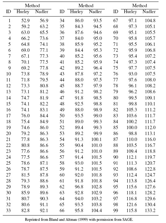
EXERCISES
1 Consider the classical linear model (1.1).
- Show that E(Y | b)= β0 + β1b and var(Y | b)= σ2e.
- Show that E(Y)= β0 + β1 µb and var(Y)= β12 σb2 + σ2ε.
Let
 1 and 2 be two replications of Y following model (1.1). That is,
where
 1 and 2 are independently distributed as e. Show that the correlation between 1 and 2 is (β12 σb2) /(β12 σ2b + σ2e). (This is the expression for reliability given in (1.4).)
2 Show that the following conditions are equivalent for perfect agreement in the paired measurements (Y1, Y2) under the assumption that σ12,σ22 > 0 :
- P(Y1 = Y2)= 1.
- {µ1 = µ2, σ12 = σ22, ρ = 1}.
- {ξ =0, τ2 = 0}.
3 Suppose (Y1, Y2) follow the measurement error model (1.6).
- Verify the expressions (1.7) and (1.8) for the mean vector and covariance matrix of (Y1, Y2).
- Verify the expressions for mean and variance of D given in (1.10).
4 Suppose for a scalar parameter φ we have two tests for the hypotheses
The first test rejects H0 if a 100(1 − α)% upper confidence bound for φ of the form ![]() + c1−α SE(
+ c1−α SE(![]() ) is less than φ0. The second test rejects H0 if the upper limit of a 100(1 − α)% two-sided confidence interval for φ of the form
) is less than φ0. The second test rejects H0 if the upper limit of a 100(1 − α)% two-sided confidence interval for φ of the form ![]() ± c1−α/2 SE(
± c1−α/2 SE(![]() ) is less than φ0. Here it is assumed that (
) is less than φ0. Here it is assumed that (![]() − φ) / SE(
− φ) / SE(![]() ) has a known distribution that is symmetric about zero for all φ, and cα is the α th percentile of this distribution.
) has a known distribution that is symmetric about zero for all φ, and cα is the α th percentile of this distribution.
- Prove that both tests have level of significance α.
- Prove that the first test is uniformly more powerful than the second test.
5 Consider the Grubbs model given in (1.19).
Show that the method of moments provides the following estimators of its parameters:

These estimators do not require the normality assumption and are called Grubbs estimators.
[Hint : Equate the mean vector and covariance matrix of (Y1, Y2), given by (1.20) and (1.21), to their sample counterparts, and solve.]- Under what conditions are the error variance estimators positive ? Do these conditions always hold?
6 Table 1.3 presents a dataset containing weights (grams) of 15 packets of potatoes measured using two kitchen scales, A and B.
Table 1.3 Potato weights (grams) data for Exercise 1.6.
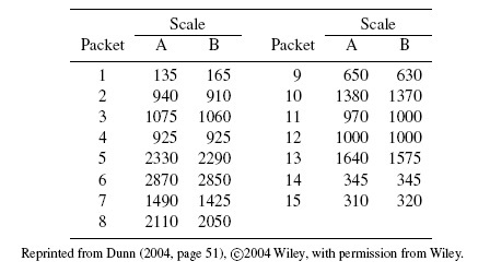
- Use Exercise 1.5 formulas to compute the Grubbs estimates for these data. What do you notice about the error variance estimates?
- Use a statistical software to fit the mixed-effects model (1.19) to these data using the ML method. What do you notice about the error variance estimates?
- Comment on the results.
7 Assuming that the paired measurements follow the measurement error model (1.18), show that the joint distribution of (D, A) is bivariate normal with mean vector
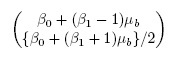
and covariance matrix
8 Table 1.4 contains measurements of inferior pelvic infundibular (IPI) angle in degrees taken from 52 kidneys using computerized tomography (method 1) and urography (method 2). Urography offers a cheaper alternative to tomography for diagnosis and treatment of kidney stones (renal lithiasis).
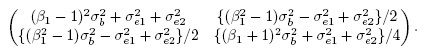
- Make a scatterplot and a Bland-Altman plot.
- Do these plots show any evidence of differences in fixed and proportional biases and precisions of the two methods?
- Is there any evidence of heteroscedasticity or of outliers?
Table 1.4 IPI angle (◦) data for Exercise 1.8.
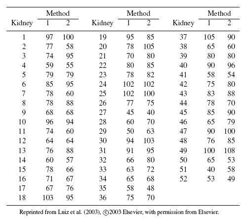
9 Table 1.5 shows the estimated fat content (g/100 ml) of human milk measured using the standard Gerber method (method 1) and a procedure that measures the amount of glycerol released by enzymic hydrolysis of triglycerides (method 2). The second method requires only 10–50 microliters of milk and is suitable for use with autoanalyzers, permitting rapid sample throughput.
- Make a scatterplot and the Bland-Altman plot for these data.
- Do these plots show any evidence of differences in fixed and proportional biases and precisions of the two methods? Explain.
- Is there any evidence of heteroscedasticity or of outliers? Explain.
- You should notice a linear trend in the Bland-Altman plot. Discuss whether the trend may be due to a difference in proportional biases or precisions or both.
- Make a ratio plot of these data. Does this plot also show a linear trend? If yes, explain what this may suggest about the cause of the trend.
- Make a Bland-Altman plot of log-transformed data. Does this plot also show a linear trend? Explain.
10 Consider the dataset presented in Bland and Altman (1986) consisting of measurements of mean velocity of circumferential fiber shortening (VCF) obtained in 100 cases by M-mode echocardiography using two methods: the standard left ventricular long axis recordings and the left ventricular short axis recordings. These data can be obtained from the book’s website.
Table 1.5 Fat content (g/100ml) data for Exercise 1.9.
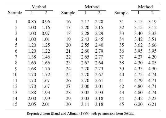
- Construct a scatterplot and the Bland-Altman plot.
- Do these plots show any evidence of differences in fixed and proportional biases and precisions of the two methods?
- Is there any evidence of heteroscedasticity or outliers?
- If you see any evidence of heteroscedasticity, make a Bland-Altman plot of log-transformed data. Does the transformation remove heteroscedasticity? Explain.
11 Consider the estimation of intercept ![]() and slope
and slope ![]() in the ordinary regression model (1.25).
in the ordinary regression model (1.25).
- Show that the estimators given in (1.26) are the least squares estimators of
 and
and  .
. - Assuming that the paired measurements follow the bivariate normal model (Section 1.12.3) and using the expressions for (,β˜1) given in (1.27), show that the least squares estimators in (a) are also the ML estimators of their respective parameters.
12 Consider the problem of fitting the line Y2 = β0 + β1 Y1 to the paired measurements using the Deming regression.
- Assume that the error variance ratio λ = 1. Show that the orthogonal least squares estimators of (β0, β1) obtained by minimizing (1.29) are (
 0,1) given in (1.30) with λ = 1.
 - Suppose λ is known and transform Y1 as
 Use part (a) to show that the orthogonal least squares estimators of the coefficients β0 and in the line
  corresponding to the transformed data (i1, Yi2) are, respectively, 0 and
- Use part (b) to show that the Deming regression line fit to the transformed data is
 Deduce that the Deming regression line fit to the original data is
13 Consider the Deming regression line of Y2 on Y1, namely, ![]() 2 =
2 = ![]() 0 +
0 + ![]() 1 Y1, where the coefficients are given by (1.30).
1 Y1, where the coefficients are given by (1.30).
- Show that the Deming regression line of Y1 on Y2 is
 1 = (− 0/1) + (1/1) Y2.
 - Deduce that there is only one Deming regression line regardless of whether Y1 or Y2 is treated as the explanatory variable.
14 (Casella and Berger, 2001, Exercise 12.4) Let ![]() 1, given by (1.30), be the estimator of the slope in the Deming regression line. It can be expressed as
1, given by (1.30), be the estimator of the slope in the Deming regression line. It can be expressed as
where λ = σe12 /σe22 is assumed to be known.
- Show that 1(λ) is an increasing function of λ if S12 < 0 and a decreasing function if S12 < 0.
- Show that
 the slope of the ordinary regression line of Y2 on Y1.
 - Show that
 the reciprocal of the slope of the ordinary regression line of Y1 on Y2.
15 Assume that the paired measurements represent a random sample from a bivariate normal distribution (Section 1.12.3). The goal of this exercise is to derive the formula (1.33) for a 100(1 − α)% confidence interval for σ22 /σ12 . We will do so by inverting the acceptance region of a level α test of hypotheses

where c is a specified positive constant.
Define
 Show that the above hypotheses are equivalent to
where the correlation between U and V is given by
Show that the sample (product-moment) correlation based on the (U, V) sample can be expressed as
Show that rejecting H0 if

provides a level α test.
Show that the acceptance region of the test in part (c) can be written as

Show that the confidence interval for σ22 /σ21 obtained by inverting the acceptance region in part (d) consists of values of w that satisfy

Show that the values of w that satisfy the condition in part (e) form the interval

(See Wang (1999) and Choudhary and Nagaraja (2005a) for related confidence intervals.)