CHAPTER 12
CATEGORICAL DATA
12.1 PREVIEW
Throughout this book our attention thus far was focussed on the problem of measuring agreement when data were observed on a continuous scale. This concluding chapter discusses the agreement problem when different raters or methods assign categories and presents basic models and measures for examining agreement. The categories could be on a nominal or an ordinal scale and there could be two or more. We discuss in detail a popular measure called kappa (κ) and examine its properties under a variety of setups including multiple raters and categories. We also illustrate the methods introduced with case studies.
12.2 INTRODUCTION
There are numerous instances of measuring agreement between two or more raters or methods or devices where the response variable is nominal or ordinal. A recent Google search of the phrase “agreement kappa” produced over 15 million hits; in the medical field alone, the search engine on the PubMed website provided links to more than 22 ,000 research papers. This problem is also frequent in the fields of psychology, education, and social sciences. In this chapter, we provide a basic introduction to the agreement problem with categorical ratings. The phrase “Cohen’s kappa” itself produced nearly 400 ,000 links on Google and about 3 ,200 papers on PubMed. Consequently, the kappa coefficient is the focus of our exploration, in spite of its shortcomings and perceived paradoxes.
First, we introduce typical categorical datasets that arise in measuring agreement with two raters and a not so widely known graph that is useful in visualizing the strength of agreement for ordinal data. We carry out an in-depth study of the properties of the kappa coefficient under a variety of settings when there are two raters and only two categories. We provide explicit expressions for the relevant parameters and their estimates, and describe associated inferential procedures, including the sample size determination. We explain the perceived paradoxes in the properties of the kappa coefficient using its mathematical properties.
Next, we investigate the problem of measuring agreement when there are two or more raters and there are more than two rating categories. We will consider both nominal and ordinal scales and the data on ordinal scale leads us to the exploration of weighted kappa coefficients and ANOVA models. We briefly touch upon the prominent modeling approaches to study agreement as well as disagreement. They include conditional logistic regression models and a generalized linear mixed-effects model approach for the dichotomous case, and log-linear models for multi-category ratings. This chapter also contains detailed case studies and a discussion on appropriate interpretation of the kappa statistic.
12.3 EXPERIMENTAL SETUPS AND EXAMPLES
12.3.1 Types of Data
While measuring agreement between two or more raters with categorical ratings, the ratings could be nominal or ordinal. With nominal ratings, a good measure of agreement treats all the disagreements between two raters equally and the entire focus is on the cases where the raters agree. In contrast, when the ratings are ordinal in nature, it becomes necessary to quantify the degree of disagreement and incorporate it into the measure of agreement. Whatever be the scale used for ratings, it also matters whether the raters involved can be treated as fixed raters or can be assumed to be randomly chosen raters. In the former case, there are two possible scenarios. The raters could be two specific raters using their own internal mechanism or two mechanisms or protocols that are followed by arbitrary rating personnel; the basic assumption is that ratings are done across randomly chosen subjects. In both these cases, there is a possibility of rater bias, in that the marginal probability that the first rater assigns a rating category of say 1 is not the same for the second rater and this bias (either due to a specific rater or due to the protocol used) affects the common measures of agreement. This leads to the fixed rater setup with a potential for rater bias and the classical Cohen’s κ . Our most basic model assumes this possibility a priori; we also consider the case where the marginal probabilities of categories are taken to be identical across raters. This second scenario can arise when randomly chosen raters are doing the rating, and this leads to the intraclass version of the κ measure. Such a situation arises when each subject is rated by two randomly chosen raters who are similarly professionally trained; for example, two radiologists interpreting the same X-ray using a similar methodology.
12.3.2 Illustrative Examples
12.3.2.1 Agreement Between Meta Analyses and Subsequent Randomized Clinical Trials
A study investigated the agreement or lack there of between meta analyses and subsequent large randomized clinical trials (involving 1000 or more subjects) published in four of the most prominent medical journals. The researchers examined altogether 40 compatible hypotheses on primary or secondary outcomes coming out of 12 large trials and 19 meta analyses. Table 12.1 provides the distribution of “Positive” or “Negative” conclusions drawn from paired cases. Here the method of using meta analysis and the method of doing a large randomized clinical trial are treated as two fixed raters.
Table 12.1 Observed conclusions of randomized clinical trials and preceding meta analyses.
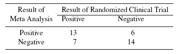
In this simple example, 27(= 13 + 14) out of the 40 or 67.5% of conclusions of preceding meta analyses agree with the large-scale randomized clinical trials that were carried out later. Given that the well-conducted meta analyses as well as the randomized trials were based on large sample sizes, we would have anticipated a higher level of agreement between them. Another perspective on this agreement statistic is obtained by asking the question: if occurred by chance alone, what would we expect in those cells that corresponded to agreement? We would have anticipated the two conclusions to agree {(20 × 19) /40 } + {(20 × 21) /40 } = 20 or 50% of the time. That is, agreement was only 17.5% beyond anticipated by chance.
12.3.2.2 Agreement Between Physicians and Nurses
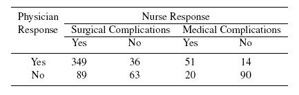
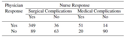
A study examined the agreement between the assessments of physicians (rater 1) and nurses (rater 2) using a retrospective chart review of 1025 Medicare beneficiaries aged 65 years or older. It compared samples of cases that were flagged by the Complications Screening Program (CSP, a computer program that screens hospital discharge abstracts for potentially substandard care) for one of 15 surgical complications and five medical complications. We consider the agreement problem for the totals of surgical and medical complications. This can be viewed as a two fixed raters problem, since physicians and nurses are trained differently.
Table 12.2 provides the distribution of the confirmation of CSP-flagged cases by the physicians and nurses on two types of complications.
Table 12.2 Summary of observed responses of physicians and nurses on medical and surgical cases flagged by the CSP system.
12.3.2.3 Multi-Category Agreement Data: Agreement in Multiple Sclerosis Assessment
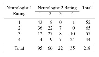
Multiple sclerosis (MS) is an autoimmune disorder affecting the central nervous system in adults with debilitating effects on the activities of their daily life. Two neurologists (one from Winnipeg, Canada, labeled 1; and the other from New Orleans, USA, labeled 2) classified two groups of patients on the certainty of MS using the following ordinal scale labeled 1 through 4 for certain (=1), probable (=2), possible (=3, with odds 1:1 ), and doubtful, unlikely, or definitely not (=4) categories. The data from the individual groups have been separately studied extensively. In Table 12.3, we pool the data and study the problem of agreement using basic models introduced in this chapter. These are two fixed raters using multi-category ratings scheme using an ordinal scale.
Table 12.3 Diagnosis by two neurologists of patients on the likelihood of multiple sclerosis.
An example of random raters and multiple nominal categories is discussed in Exercise 12.17.
12.3.3 A Graphical Approach
Bangdiwala introduced a chart that illuminates the inter-rater bias as well as the strength of agreement between two raters. It provides a simple, powerful visual assessment of both inter-rater bias and agreement within ordinal categories.
Suppose two raters are classifying n subjects on an ordinal scale into one of c categories labeled 1 ,...,c , and the data are arranged in the form of a c × c contingency table. Let nij , frequency of the (i, j)th cell, represent the number of subjects who were classified into category i by rater 1 and j by rater 2. Denote by ni · and n·j the total frequency of the ith row and j th column, respectively, for i, j = 1, ..., c. Further, define n0· = n·0 = 0, and partial sums ![]()
The agreement chart is constructed using the following steps:
- Draw an n × n square and a 45◦ reference line.
- Draw c rectangles Ri, i = 1,..., c, inside the square such that Ri has dimension ni· × n·i. These rectangles are placed sequentially inside the n × n square such that rectangle Ri has lower left vertex at (si−1· ,s·i−1) , and upper right vertex at (si· ,s·i) , for i = 1, ..., c. Note that if either ni· or n·i is zero, then Ri reduces to a vertical or horizontal line.
- Divide Ri into a c × c grid where the embedded nij × nki rectangle r(j, k) corresponding to the (j, k)th grid has lower left vertex at
 and upper right vertex at
- Within ri shade the region r(j, k) based on the values of l = max {| j − i |, | k − i |} where the intensity of the shade is a strictly decreasing function of l. The nii × nii square region r(i, i) corresponding to the (i, i) th grid (and l = 0 ) is the region of perfect agreement and will have the darkest shade.
- Repeat Steps 3 and 4 for i = 1,..., c with the same choice of shading levels.
If there is very limited inter-rater bias, the ni· and n·i remain close and hence the rectangle Ri comes close to being a square. When this happens for most of the i, the rectangles come close to the reference line in the original n × n square. As the inter-rater bias becomes more pronounced, the rectangles move farther away from the diagonal and can move either below or above it. The shading pattern within the i th rectangle provides an insight into the level of agreement as well as of disagreement when at least one of the raters has classified a subject into category i. The agreement chart can be drawn with multi-category nominal data, but then the shading pattern would not correlate with the magnitude of disagreement and hence becomes less informative.
Figure 12.1 provides the agreement chart for the multi-category ordinal MS data introduced in Section 12.3. The numbers along the top and right edges of the outer square represent, respectively, the total frequencies corresponding to the four ratings of Neurologists 1 and 2. Discrepancies in the marginal frequencies of the two neurologists for categories 1, 3, and 4 lead to non-square shapes. For category 2, we obtain nearly a square due to the closeness of the marginal frequencies, but even then, the full agreement is limited there as shown by the small black square within it.
12.4 COHEN’S KAPPA COEFFICIENT FOR DICHOTOMOUS DATA
Consider a sample of n subjects or specimens that are classified into one of two categories labeled 1, 2 by J raters. Let Yij denote the rating of the ith subject by the jth rater; j = 1,..., J. We assume that (Yi1, ..., YiJ ), i = 1,..., n form a random sample from the joint distribution of (Y1,...,YJ) over the j-dimensional cube {1, 2}J. The interest is to assess the agreement of two raters taken in pairs and to obtain a summary measure of agreement that provides an overall measure for the group of J raters. Cohen’s kappa coefficients, introduced in 1960 for two raters classifying into two categories and generalized to several raters and multiple categories in later years, provide commonly used measures for this purpose. We introduce these measures, and study their properties under suitable models with the goal of providing measures for intra-rater as well as inter-rater agreement. We take up the two raters case first; that is, take J = 2.
12.4.1 Definition and Basic Properties: Two Raters
Let (Y1,Y2) have the joint pmf and marginal pmfs of Y1 and Y2 given, respectively, by
 (12.1)
The parameter space for this multinomial trial is
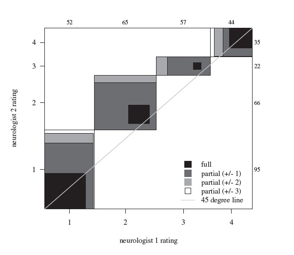
Figure 12.1 Bangdiwala agreement chart for the MS data in Table 12.3.
Then a simple metric for measuring agreement is the probability
 (12.2)
Note that 0 ≤ θ ≤ 1, and θ is 0 when p11 = p22 = 0 leading to perfect disagreement, and is 1 when p12 = p21 = 0 leading to perfect agreement. In both these extreme cases, the joint distribution has at most two points in its support.
There can be an agreement between the two raters even if they were choosing categories randomly. To adjust for this, Cohen proposed a measure that is corrected for chance by introducing the probability of such an event due to random causes,
 (12.3)
The parameter θ0 is also between 0 and 1, and θ0 is 0 when p12 or p21 is 1 (with perfect disagreement), and it is 1 when p11 or p22 is 1 with perfect agreement. In both the extreme cases, however, the joint distribution is degenerate.
Cohen’s kappa measure is then given by
 (12.4)
where we assume that θ0 < 1. Clearly, κ ≤ θ ≤ 1 and when θ0 is specified, κ ≥ −(1 − θ0)−1 ≥−1. Further, κ = 0 only when θ = θ0 or when P (Y1 = Y2) remains the same as due to chance. Upon substituting for θ and θ0 in terms of the pij and simplifying the right-hand side of (12.4) we obtain
 (12.5)
This form suggests that κ = 0 if and only if the odds ratio O R = p11 p22 /p12 p21 = 1. Further, it expresses κ as an explicit function of the multinomial probabilities. Hence ![]() , the ML estimator of κ, can be computed from the ML estimators of the pij and an expression for the standard error of
, the ML estimator of κ, can be computed from the ML estimators of the pij and an expression for the standard error of ![]() can be given using the well-known asymptotic properties of the ML estimators. Details are given in the next section.
can be given using the well-known asymptotic properties of the ML estimators. Details are given in the next section.
There are numerous investigations in the psychology and medical literature that discuss different scenarios where the raw agreement metric θ is high, but κ is very low and even negative. To explain this phenomenon with mathematical clarity, we will reparameterize the space of the pij by writing
 (12.6)
where δ1 represents the magnitude of asymmetry when there is agreement and δ2 represents a similar discrepancy measure when there is a disagreement between the two raters. The corresponding parameter space is

In terms of these parameters, it follows that
 (12.7)
With ![]() . For a fixed θ , κ (x) is increasing in x (Exercise 12.3). Consequently,
. For a fixed θ , κ (x) is increasing in x (Exercise 12.3). Consequently,
 (12.8)
provide lower and upper limits for the possible values of κ for a given probability of agreement θ. Figure 12.2 provides these bounds as θ moves in (0, 1). It shows that even in the best case scenario, κ remains small for θ under 0.80. Further, even when θ is close to 1, it is possible to have κ being negative, and it happens when p21 = p12 while either p11 or p22 remains close to θ.
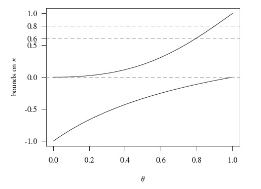
Figure 12.2 Range of κ values for a given probability of agreement θ. Given θ = 0.8, κ cannot exceed 0.6; even when θ is as high as 0.90, κ cannot exceed 0.8, and can be negative.
Another useful parameterization of the parameter space with κ as a component exists. It can be used to further explore bounds on κ. With θ1 = p11 + p12 ≡ p1·, θ2 = p11 + p21 ≡ p·1, the pij can be expressed in terms of θ1, θ2, and κ as:
 (12.9)
Non-negativity of the pij leads to further bounds on κ in terms of θ1 and θ2. The parameter space ![]() is equivalent to the space
is equivalent to the space

where (Exercise 12.4)
 (12.10)
There are two other forms for κ defined in (12.4). To develop them, first consider
Let µ j = E(Yj ) and σ j2 = var(Yj), j = 1, 2. Then
upon simplification. This leads to another important form for the κ coefficient given by
 (12.11)
where ρ is the Pearson correlation of Y1 and Y2. In this form, Cohen’s kappa can be seen as the concordance correlation coefficient (CCC) introduced in (2.6) of Section 2.4. The form in (12.11) also shows that when p·2 = p2· or equivalently when p12 = p21 or when Y1 and Y2 are identically distributed, κ = ρ; in other cases it is smaller than ρ.
There is another easily interpretable representation for 1 − θ0 that can be used to give yet another expression for κ; see Exercise 12.5.
12.4.2 Sample Kappa Coefficient
The original multinomial parameterization with expression for κ given in (12.5) leads us to simple forms for the ML estimator ![]() . Suppose we have n subjects being classified by raters 1 and 2. As in Section 12.3.3, let nij denote the number of subjects being classified into category i by rater 1 and j by rater 2, i, j = 1, 2. Let
. Suppose we have n subjects being classified by raters 1 and 2. As in Section 12.3.3, let nij denote the number of subjects being classified into category i by rater 1 and j by rater 2, i, j = 1, 2. Let ![]() and
and ![]() The data are usually tabulated as in Table 12.4. We assume that the n subjects being rated form a random sample from the multinomial population. Thus, the log-likelihood function is given by
The data are usually tabulated as in Table 12.4. We assume that the n subjects being rated form a random sample from the multinomial population. Thus, the log-likelihood function is given by
and consequently the ML estimator of pij is ![]() ij = nij /n. By the invariance property of the ML estimators, the ML estimator of κ represented by (12.5) is given by
ij = nij /n. By the invariance property of the ML estimators, the ML estimator of κ represented by (12.5) is given by
 (12.12)
Table 12.4 Summary of observed responses of raters 1 and 2.
We can use the other forms of κ given above and write down the corresponding equivalent forms for ![]() . A large-sample estimate of var(
. A large-sample estimate of var(![]() ) is given by
) is given by
 (12.13)
where ![]() 0 is the ML estimator of θ0 defined in (12.3), and
0 is the ML estimator of θ0 defined in (12.3), and ![]() is given by (12.12). This estimate along with the assumption of normal approximation to the distribution of
is given by (12.12). This estimate along with the assumption of normal approximation to the distribution of ![]() can be used to find large-sample confidence bounds and intervals for κ as well as to test the agreement hypotheses (of common interest) of the form (1.13), H0 : κ ≤ κ 0 versus H1 : κ > κ0. For example, the fact that
can be used to find large-sample confidence bounds and intervals for κ as well as to test the agreement hypotheses (of common interest) of the form (1.13), H0 : κ ≤ κ 0 versus H1 : κ > κ0. For example, the fact that
approximately, can be used to suggest ![]() lower confidence bound for κ.
lower confidence bound for κ.
For the meta analysis and randomized clinical trial agreement example in Section 12.3.2.1, the cell frequencies are n11 = 13, n12 = 6, n21 = 7, and n22 = 14. Consequently, the sample kappa coefficient ![]() given in (12.12) turns out to be 0 .35 with an estimated standard error of 0.1479 upon using the formula in (12.13). The associated lower confidence bound of 0.1067 has an approximate confidence level of 95%.
given in (12.12) turns out to be 0 .35 with an estimated standard error of 0.1479 upon using the formula in (12.13). The associated lower confidence bound of 0.1067 has an approximate confidence level of 95%.
But the coverage level for the above confidence bound can vary from the nominal level 100(1 − α )% even for n = 100 for some combinations of κ, pi·, and p·i. Hence we recommend confidence bounds and intervals based on bootstrapping for small sample sizes.
12.4.3 Agreement with a Gold Standard
Now suppose rater 1 is the gold standard. Then there are measures of agreement other than κ that are relevant and readily interpretable. By taking response category of 1 as positive, the commonly used measures are the conditional probabilities sensitivity η1 and specificity η2, given, respectively, by
 (12.14)
where θ1 ≡ p1· is the prevalence parameter. Then κ can be expressed in terms of these parameters as (Exercise 12.6)
 (12.15)
When η1 and η2 are known, κ will be a function of prevalence θ1, and its maximum possible value is given by
 (12.16)
12.4.4 Unbiased Raters: Intraclass Kappa
In the kappa coefficient introduced above, there was no constraint on the propensity of the two raters to classify the same proportion of subjects into any specific category; that is, we assumed that inter-rater bias may exist. In certain situations, an assumption of no inter-rater bias appears reasonable. One is where the same rater rates a subject twice, as in a repeatability study, and the other is the case where we can draw a random sample of two raters from the available raters and use their ratings of the same subject. In both these cases, we can assume unbiasedness of two raters. In the first case, the agreement problem corresponds to intra-rater reliability, and in the second, the concern is about inter-rater reliability. Thus, with unbiased raters, we are lead to a situation where the parameter space is restricted by the condition p·1 = p1· or, equivalently, p12 = p21, or the case where δ2 = 0, or the assumption that Y1 and Y2 are identically distributed. Further, the expression for κ simplifies to
 (12.17)
which is nothing but the correlation between Y1 and Y2 where the two random variables are now exchangeable. This conclusion also follows from the CCC form for κ given in (12.11). Thus, κ can be identified as the intraclass correlation coefficient when the raters are unbiased. This interpretation is particularly helpful in the case of randomly chosen multiple raters.
It is convenient to use the parameters θ, δ1, and δ2 introduced in (12.6) and take δ2 = 0 to describe κI using (12.7), and also to express the likelihood for the observed data. For a random sample of n subjects, the log-likelihood is given by

Consequently, the ML estimators under the restricted parameter space are
Hence we conclude that, for the unbiased raters model, the population κ coefficient is
 (12.18)
is its ML estimator. An approximation to the variance of the sample intraclass κ is given by
 (12.19)
where ![]() I is given in (12.18), and
I is given in (12.18), and
These ML estimators assume the exchangeability of Y1 and Y2.
12.4.5 Multiple Raters
Suppose there are J (≥ 2) raters that classify each of the n subjects into one of two categories labeled 1 and 2. Let Yij be the rating of the ith subject by the jth rater, j = 1,...,J; i = 1,...,n. Define Bernoulli random variables Yij∗ as
We assume the sample of n subjects is randomly chosen. The agreement question for two raters can be generalized to this setup and we consider two models for this purpose. They are, respectively, the fixed rater and random rater models.
If the goal is measuring agreement between the specified J raters, one can find sample κ for each of the ![]() pairs using (12.12) and take the average κ as the estimate of the assumed common κ value. One can simplify this task by grouping the subjects based on the number of positive classifications. In addition, we can use the jackknife procedure to reduce bias in the estimate. We can find the confidence intervals and bounds using bootstrapping by resampling the n subjects, and carry out hypothesis testing using this approach.
pairs using (12.12) and take the average κ as the estimate of the assumed common κ value. One can simplify this task by grouping the subjects based on the number of positive classifications. In addition, we can use the jackknife procedure to reduce bias in the estimate. We can find the confidence intervals and bounds using bootstrapping by resampling the n subjects, and carry out hypothesis testing using this approach.
When there are multiple raters, one can also test for the rater bias using Cochran’s Q test. It is implemented as follows. First define
 (12.20)
The absence of rater bias corresponds to the null hypothesis that ![]() are the same for j = 1 ..., J. The test statistic used is
are the same for j = 1 ..., J. The test statistic used is
 (12.21)
where it is assumed that there is at least one pair of disagreement in the dataset so that the denominator is nonzero. Under the null hypothesis of no bias across raters, Q has an approximate χ2 distribution with (J − 1) degrees of freedom. When j = 2, the resulting test reduces to the McNemar’s test. Conclusions drawn from this test for homogeneity of the raters can be incorporated into the overall estimate of κ.
When ![]() are assumed to be the same for j = 1 ..., J, one can consider the intraclass correlation interpretation for κ under a random effects model (that makes additional assumptions) to obtain an estimate for it. We will discuss that model next.
are assumed to be the same for j = 1 ..., J, one can consider the intraclass correlation interpretation for κ under a random effects model (that makes additional assumptions) to obtain an estimate for it. We will discuss that model next.
The one-way random effect model that assumes an exchangeable dependence structure for the ratings on a subject is natural when we have J randomly drawn raters. Let us assume that the Bernoulli variables Yij∗ can be expressed as
 (12.22)
where the independent random variables si and eij have zero means and variances σ2s and σ2e, respectively. Then the intraclass correlation, that is, the correlation between any two measurements on subject i is σ2s /(σ2s + σ2e). Upon recalling (12.17), we note that this is another representation for κ under the assumptions of the model in (12.22). Following the familiar approach used in the normality-based ANOVA models we can use moment estimators of the variance components to obtain another estimator for the intraclass kappa, κI. The unbiasedness of the moment estimators of the variance components do not depend on normality. Define the between subject mean square (BMS) and within subject mean square (WMS) as follows:
 (12.23)
where ![]() are defined in (12.20). Then it can be shown that (Exercise 12.10)
are defined in (12.20). Then it can be shown that (Exercise 12.10)
 (12.24)
Thus, ![]() can be estimated by
can be estimated by
 (12.25)
The above approach has assumed that raters’ classifications of different subjects are independent. Thus, it can be used even when the subjects are evaluated by varying number of raters that are possibly different as long as our assumption that the model given in (12.22) holds.
There are other approaches to estimating κI, such as jackknifing, that avoid the ANOVA approach. One can also use the bootstrap estimate of κI and find the lower confidence limit from the resampled distribution. We recommend this approach to find the confidence limit as the convergence to large-sample properties is very slow.
12.4.6 Combining and Comparing Kappa Coefficients
Suppose there are m experiments comparing two raters (or two methods of classification), each classifying the subjects into one of two categories, and the experiments produce independent estimates of κ. This is a typical scenario in a meta analysis context. Another scenario is when we have the marginal probabilities of classification that may depend on confounding variables and they vary across the experiments.
Let κj be the population parameter corresponding to the jth experiment and let ![]() j be the associated sample κ coefficient based on a sample of size nj, j = 1,...,m. Under the assumption that the κ j are all the same and their common value is κ∗, its estimate is given as a weighted sum by the following formula,
j be the associated sample κ coefficient based on a sample of size nj, j = 1,...,m. Under the assumption that the κ j are all the same and their common value is κ∗, its estimate is given as a weighted sum by the following formula,
 (12.26)
where ![]() j is computed using the formula for
j is computed using the formula for ![]() given in (12.12). One can consider two choices for the weights Cj. One is Cj = nj, and another is
given in (12.12). One can consider two choices for the weights Cj. One is Cj = nj, and another is ![]() is computed using the formula in (12.13). The motivation for considering the second set of weights comes from the optimal estimation of the common mean using independent estimators with different variances. One can also consider pooling the data (if available) and then computing the sample kappa coefficient for the combined sample of size
is computed using the formula in (12.13). The motivation for considering the second set of weights comes from the optimal estimation of the common mean using independent estimators with different variances. One can also consider pooling the data (if available) and then computing the sample kappa coefficient for the combined sample of size![]() Simulation has shown that weighting by the sample sizes (i.e., taking Cj = nj) produces estimates of κ∗ that have smaller bias and mean square error under a variety of settings, including when sample sizes are small.
Simulation has shown that weighting by the sample sizes (i.e., taking Cj = nj) produces estimates of κ∗ that have smaller bias and mean square error under a variety of settings, including when sample sizes are small.
A test of the null hypothesis that the κj are all the same can be constructed using the test statistic T given by
 (12.27)
where, ![]() * is computed from (12.26) with
* is computed from (12.26) with ![]() Under the null hypothesis T has approximately X2 distribution with (m − 1) degrees of freedom, and the hypothesis is rejected for large values of T. This works well when the sample sizes are large (> 100).
Under the null hypothesis T has approximately X2 distribution with (m − 1) degrees of freedom, and the hypothesis is rejected for large values of T. This works well when the sample sizes are large (> 100).
When one can assume that the raters are unbiased in each of the m experiments, we can use the intraclass kappa coefficient κI as the measure of agreement. Under this model, using ![]() I in place of
I in place of ![]() and taking
and taking ![]() , where the variance estimate is given by (12.19) in the statistic T defined in (12.27), leads to a χ2 test statistic that has better power properties for smaller sample sizes. One can also consider the problem of testing the equality of two dependent κ coefficients with two raters and two categories under this intraclass kappa model. With additional modeling assumptions, one can present a test that is similar in spirit to the test statistic T presented for the comparison of independent κ coefficients, but modified to account for the dependence between the two kappa estimates.
, where the variance estimate is given by (12.19) in the statistic T defined in (12.27), leads to a χ2 test statistic that has better power properties for smaller sample sizes. One can also consider the problem of testing the equality of two dependent κ coefficients with two raters and two categories under this intraclass kappa model. With additional modeling assumptions, one can present a test that is similar in spirit to the test statistic T presented for the comparison of independent κ coefficients, but modified to account for the dependence between the two kappa estimates.
12.4.7 Sample Size Calculations
Consider the problem of measuring agreement between two raters or methods that categorize a given subject into one of two categories. Suppose one wants to test the null hypothesis H0 : κ = κ0 versus the one-sided alternative H1 : κ > κ0 at level of significance α, and wants a power of 100(1 − β)% at κ = κ1(> κ0). Typically, one would use the large-sample normal approximation to obtain the sample size
 (12.28)
where ![]() is an estimate of var(
is an estimate of var(![]() ) with
) with ![]() being the sample κ given in (12.12). Further, z1−α and z1−β are the 100(1 − α)th and 100(1 − β)th percentile of the standard normal distribution. From the large-sample approximation to
being the sample κ given in (12.12). Further, z1−α and z1−β are the 100(1 − α)th and 100(1 − β)th percentile of the standard normal distribution. From the large-sample approximation to ![]() , given in (12.13), it is clear that the variance estimate depends on estimates of several parameters including κ. With the reparameterization of the cell probabilities in terms of κ, and marginal probabilities p1· and p·1, given in (12.9), it follows that the expression for
, given in (12.13), it is clear that the variance estimate depends on estimates of several parameters including κ. With the reparameterization of the cell probabilities in terms of κ, and marginal probabilities p1· and p·1, given in (12.9), it follows that the expression for ![]() depends on estimates for these three parameters of which κ is the parameter of interest. So, one could use preliminary estimates of p1· and p·1 from a pilot sample or prior prevalence studies in the formula for
depends on estimates for these three parameters of which κ is the parameter of interest. So, one could use preliminary estimates of p1· and p·1 from a pilot sample or prior prevalence studies in the formula for ![]() and substitute κ0 and κ1 to choose the larger of the two estimates as
and substitute κ0 and κ1 to choose the larger of the two estimates as ![]() . Then the use of (12.28) yields the desired sample size. As we have seen before in (12.10), the choices for p1· and p·1 restrict the range for κ and one needs to choose them so that both κ0 and κ1 are feasible under these constraints. If it is appropriate to assume unbiasedness of raters (say when raters are randomly chosen), we use
. Then the use of (12.28) yields the desired sample size. As we have seen before in (12.10), the choices for p1· and p·1 restrict the range for κ and one needs to choose them so that both κ0 and κ1 are feasible under these constraints. If it is appropriate to assume unbiasedness of raters (say when raters are randomly chosen), we use ![]() I defined in (12.18) to carry out the test and take
I defined in (12.18) to carry out the test and take ![]() from the variance approximation given in (12.19) to compute n using (12.28). With appropriate modifications, the sample size formula in (12.28) can be used for tests involving agreement measures for continuous measurements. See Exercise 12.20.
from the variance approximation given in (12.19) to compute n using (12.28). With appropriate modifications, the sample size formula in (12.28) can be used for tests involving agreement measures for continuous measurements. See Exercise 12.20.
We recommend the use of simulation studies for sample size calculations, especially for more complex setups.
12.5 KAPPA TYPE MEASURES FOR MORE THAN TWO CATEGORIES
12.5.1 Two Fixed Raters with Nominal Categories
When there are c (≥ 3) categories and J = 2 raters, the joint pmf of their ratings of a subject is given by (12.1), where now the possible ratings i, j by the two raters belong to the set {1, 2,...,c}. Then, the κ coefficient, introduced in (12.4) takes on the form
 (12.29)
where now θ0, the probability of agreement due to chance, is ![]() The ML estimation methodology here follows the description given in Section 12.4.2 and will not be presented.
The ML estimation methodology here follows the description given in Section 12.4.2 and will not be presented.
While the above approach directly generalized the definition of κ in the dichotomous case as a chance adjusted measure of agreement, the available data also provides an opportunity to examine the agreement measure for individual categories. Let κt be the kappa coefficient obtained by dichotomizing the categories as t versus non-t, for t = 1,..., c. The estimates of κt will provide an idea about the variation in the agreement between the two raters in terms of the choice of a particular category. In fact, the overall κ defined above in (12.29) is a weighted sum of these κt. It can be shown that ![]() , where the weight
, where the weight
 (12.30)
is non-negative and ![]() See Exercise 12.11.
See Exercise 12.11.
When there are multiple categories, the kappa coefficient just discussed treats all disagreements equally and in fact ignores them completely. But when categories are ordered, the magnitudes of disagreement can be quantified in some cases using a suitably chosen weight function. In such situations a weighted κ, introduced below, provides a more meaningful measure of agreement.
12.5.2 Two Raters with Ordinal Categories: Weighted Kappa
Suppose there are c ordered categories labeled 1,..., c and let wij denote the agreement weight associated with the classification i by rater 1 and j by rater 2; i, j = 1,..., c. Take wii = 1 for perfect agreement, and for j ≠ i, 0 ≤ wij < 1 for imperfect agreement; further assume wij = wji. Then the weighted κ is defined by
 (12.31)
Since the wij are bounded by 1, both the weighted sums in the second form are positive, and consequently κw does not exceed 1. The last form also shows that a scale change in (1 − wij) will not alter the value of κw.
The ML estimators for the parameters in (12.31) are ![]() ij = nij /n,
ij = nij /n, ![]() i· = ni· /n, and
i· = ni· /n, and ![]() ·j = n·j /n. Using these, the ML estimator of κw,
·j = n·j /n. Using these, the ML estimator of κw, ![]() w, can be computed. A close large-sample approximation to its variance estimate is given by
w, can be computed. A close large-sample approximation to its variance estimate is given by
 (12.32)
where ![]() i· is the average weight given to category i (recall that
i· is the average weight given to category i (recall that ![]() i· =
i· = ![]() ·i due to the symmetry of the weight function) and
·i due to the symmetry of the weight function) and
Two weight functions based on squared distance and absolute distance are generally used. As expressed in the form of disagreement weights, they are given by
 (12.33)
When pi· = p·i for all i and 1 − wij ∝ (i − j)2, κw is identical to the Pearson correlation between the ratings of the two raters (Exercise 12.12).
When 1 − wij ∝ (i − j)2, the sample estimate ![]() w is very close (at the order of 1 /n) to the moment estimate of the intraclass correlation coefficient in a two-way random effects model where the two raters as well as the subjects are treated as random effects and the observations are the numerical ratings with support {1,...,c}. Note that the random effects model assumption here causes the two rating distributions to be exchangeable. Thus, the standard techniques associated with the ANOVA table applicable to two-way ANOVA can be employed to get quick estimates of κw. This approach is further discussed in Section 12.5.3 below.
w is very close (at the order of 1 /n) to the moment estimate of the intraclass correlation coefficient in a two-way random effects model where the two raters as well as the subjects are treated as random effects and the observations are the numerical ratings with support {1,...,c}. Note that the random effects model assumption here causes the two rating distributions to be exchangeable. Thus, the standard techniques associated with the ANOVA table applicable to two-way ANOVA can be employed to get quick estimates of κw. This approach is further discussed in Section 12.5.3 below.
When wij = 1 for i = j and 0 otherwise, the weighted kappa reduces to κ, given in (12.29).
12.5.3 Multiple Raters
When there are c (≥ 3) categories and J (≥ 3) raters, extensions of the kappa coefficient discussed so far do exist. There are several variance components models that make numerous assumptions. But the interpretation of the estimates of agreement coefficients becomes less clear in most cases. These generally involve the intraclass correlation interpretation of κ and make the assumption of random raters.
Suppose the J raters are distinct across subjects being rated and there are c categories. We suggest the use of pairwise κw defined in (12.31) across the J raters, and their average as an overall measure of agreement. Lower confidence bounds can be obtained using the recommended bootstrapping approach.
When the raters can be taken to be random effects, a two-way random effects model given by
 (12.34)
can be fit where Yij is the rating given by rater j for subject i and takes on values 1,..., c (≥ 2). This is a generalization of the model proposed in (12.22) and assumes that the raters are unbiased and rj has a constant variance ![]() . The intraclass correlation that corresponds to the inter-rater agreement is then given by
. The intraclass correlation that corresponds to the inter-rater agreement is then given by
 (12.35)
This reduces to the weighted κ coefficient introduced above in Section 12.5.2 when J = 2, the raters are exchangeable, and the weight function chosen is wij = 1 −{(j − i) /(c −1)}2. The intraclass correlation ρC can be estimated using standard ANOVA methods that involve variance component estimates and let ![]() C be its estimate obtained by plugging in the moment estimates of these variance components. Then the variance of
C be its estimate obtained by plugging in the moment estimates of these variance components. Then the variance of ![]() C can be approximated by
C can be approximated by
 (12.36)
In the above approximation, the estimates of the variance components as well as their variances and covariances are obtained from the fitted model.
For finding a confidence bound for ![]() C, we can use the methodology already available for the usual two-way ANOVA model with random effects. See Exercise 12.16.
C, we can use the methodology already available for the usual two-way ANOVA model with random effects. See Exercise 12.16.
12.6 CASE STUDIES
12.6.1 Two Raters with Two Categories
Consider the dichotomous classification of physicians and nurses of 1025 Medicare beneficiaries introduced in Section 12.3.2.2. Two types of complications were considered for determining the degree of agreement.
For decisions on surgical issues, 71.69% of the physicians and 81.56% of the nurses found complications and McNemar’s χ2 test that tests for symmetry of disagreement or equivalently H0 : p1· = p·1 strongly rejects it with a p-value of under 0.0001. The sample kappa, ![]() , given by (12.12), is 0.3588 and the 95% lower confidence limit based on the variance estimate in (12.13) and asymptotic normality is 0.2847. This is a situation where there is a rater bias and the sample kappa value is low even though the physicians and nurses agree on 76.72% of the cases examined.
, given by (12.12), is 0.3588 and the 95% lower confidence limit based on the variance estimate in (12.13) and asymptotic normality is 0.2847. This is a situation where there is a rater bias and the sample kappa value is low even though the physicians and nurses agree on 76.72% of the cases examined.
For decisions on medical complications, 37.14% of the physicians and 40.57% of the nurses responded “Yes.” McNemar’s χ2 test that tests H0 : p1· = p·1 fails to reject it with a p-value of 0.3035 . The sample kappa, ![]() , given by (12.12), is 0.5916. Had we assumed no rater bias and used the maximum likelihood estimate of the intraclass version of kappa using (12.18),
, given by (12.12), is 0.5916. Had we assumed no rater bias and used the maximum likelihood estimate of the intraclass version of kappa using (12.18), ![]() I would have been 0.5911. The 95% lower confidence limit based on the variance estimate in (12.13) and the assumption of asymptotic normality is 0.4889. This is a situation where there is hardly any rater bias and the sample kappa value is higher; further, the physicians and nurses agree on 80.57% of the cases examined.
I would have been 0.5911. The 95% lower confidence limit based on the variance estimate in (12.13) and the assumption of asymptotic normality is 0.4889. This is a situation where there is hardly any rater bias and the sample kappa value is higher; further, the physicians and nurses agree on 80.57% of the cases examined.
12.6.2 Weighted Kappa: Multiple Categories
In Section 12.3.2.3, we introduced an example on agreement between two neurologists where the ratings were measured on an ordinal scale. Earlier, we provided a graphical representation using Bangdiwala’s agreement graph for these data in Section 12.3.3.
The sample kappa coefficient for the multi-category (c = 4) rating scale is 0.2570 with an estimate of the standard error of 0.0429. This does not indicate a good level of agreement between the two neurologists in their classification of the 218 cases presented. Neurologist 1 (from Winnipeg) has classified 23.9%, 29.8%, 26.1%, and 20.2% of the patients into categories 1, 2, 3, and 4, respectively. In contrast, the corresponding proportions for the second neurologist (from New Orleans) are 43.6%, 30.3%, 10.1%, and 16.1%. These marginal sample proportions may tempt one to naively infer that Winnipeg and New Orleans neurologists disagree a lot while classifying a patient into either category 1 or 3; but perhaps agree to a substantial extent with category 2 or 4. A look at Table 12.3 in Section 12.3.2.3 indicates that, in the case of category 2, there is substantial disagreement; 36 of the subjects identified as category 2 by the first neurologist have been rated as 1 by the second. When we compute the kappa coefficients by dichotomizing the categories as t versus non-t, t = 1, 2, 3, and 4, the corresponding sample kappa coefficients are 0.4001, 0.0507, 0.0666, and 0.5221, respectively. These values indicate that the two neurologists agree the most when there is extreme evidence while showing hardly any agreement beyond chance in the intermediate cases.
Since we have ordinal ratings, it is very appropriate that weighted kappa coefficient be used to assess the degree of agreement between the two neurologists. With absolute distance weight function (given in (12.33)), ![]() w = 0.4406 and its estimated standard error is 0.0413. With quadratic weight function in (12.33), the estimate of
w = 0.4406 and its estimated standard error is 0.0413. With quadratic weight function in (12.33), the estimate of ![]() w and its estimated standard error are 0.5887 and 0.0459, respectively. When compared to the simple (unweighted) κ estimate of 0.2570, we see substantial increase in these estimates, but the standard error estimates remain quite stable. A random effect ANOVA model with ratings as the response variable provides an estimate of 0.5891 for the intraclass correlation coefficient; as anticipated it is very close to the
w and its estimated standard error are 0.5887 and 0.0459, respectively. When compared to the simple (unweighted) κ estimate of 0.2570, we see substantial increase in these estimates, but the standard error estimates remain quite stable. A random effect ANOVA model with ratings as the response variable provides an estimate of 0.5891 for the intraclass correlation coefficient; as anticipated it is very close to the ![]() w obtained from the use of the quadratic weight function.
w obtained from the use of the quadratic weight function.
12.7 MODELS FOR EXPLORING AGREEMENT
12.7.1 Conditional Logistic Regression Models
Suppose there are two raters where each one classifies a subject into one of two categories. We considered this situation in Section 12.4 where the kappa coefficient was introduced. There we assumed that the subjects form a random sample or that the joint probabilities pij remain the same across the subjects. But the classification probabilities may depend on known covariates. Now we present a simple model that assumes the following: (i) κ remains constant across the subjects, (ii) the marginal probabilities p1· and p·1 are the same for each subject but these probabilities vary across subjects; and (iii) the logit function log {p1· /(1 − p1·)} is related to the covariates through a linear relationship. With p1· = p·1 = θ1, we use the reparameterization defined in (12.9) to obtain
 (12.37)
Since the discordant probabilities are the same, the 2 × 2 cells in our multinomial trial can be reduced to three categories by combining the two discordant cells. To elaborate, we assign subjects with both ratings of 1 to cell 1, with discordant ratings to cell 2, and with both ratings of 2 to cell 3 with respective probabilities ![]() and (1 − θ1)2 + κθ1(1 − θ1).
and (1 − θ1)2 + κθ1(1 − θ1).
For a subject i, let Vil = 1 if the subject is placed in cell l, and 0 otherwise, for l = 1, 2, 3, and i = 1,..., n. Further, let xi = (1, xi1,..., xip)T be the covariate vector associated with the ith subject and it is related to the probability θ1 above such that
Here κ is the parameter of our interest while β = (β0,...,βp)T is the nuisance parameter vector in the problem. The multinomial likelihood is given by
This multinomial like lihood is equivalent to that of a conditional logistic regression model arising in a matched case-control study. For that representation, three observations are created for each subject i, and the outcome variable indicates which of the three cells l (l = 1, 2, 3) actually was realized; that is, the one for which Vil = 1. The observation l that corresponds toVil = 1 is taken as the case, and the other two are labeled as control. To describe the relative risk function for the underlying conditional logistic model, define covariate zi = xi, 0,– Xi, and wi = 1, −2, 1, respectively, for l = 1, 2, 3 for the ith subject. The relative risk function for that subject is then given by
 (12.38)
Software available for the conditional logistic models can then be used to obtain estimates of κ and its standard error.
12.7.2 Log-Linear Models
When the number of categories c exceeds 2, log-linear models have been used to explore the nature of agreement and association. We now introduce two simple models that are useful for the exploration of agreement for the nominal and ordinal categories.
As before, let pij denote the joint probability of a subject being rated as category i and j, respectively, by the first rater (A) and second rater (B) for i, j = 1,..., c. In the c × c contingency table, resulting from n subjects, let µij = npij denote the expected frequency in the (i, j)th cell. Consider the log-linear model
 (12.39)
where
The parameter δi included for the (i, i)th diagonal cell represents agreement beyond expected by chance for category i if raters A and B were to independently choose that category. Now if δi = δ for all i, the parameter δ can be viewed as a single measure of agreement beyond chance and can be used as a measure in place of κ. The measure δ has an interesting connection to log(τij) where
 (12.40)
For i ≠ j the numerator in the second form for τij in (12.40) represents the odds that the rating by A is i rather than j when the rating by B is i and the denominator is nothing but the odds that the rating by A is i rather than j when the rating by B is j. Under the model given by (12.39) with δi = δ, log(τij)= 2δ. Thus, δ has another meaningful interpretation as an agreement measure. Its estimation and associated inference based on ML method can be carried out using commonly available log-linear model procedures in the statistical packages.
When categories are ordinal in nature, a parsimonious model that would account for a measure of agreement and a linear-by-linear association is given by
 (12.41)
where 0 < u1 < ... < uc are fixed scores assigned to the c categories and δij = δ for i = j and is 0, otherwise. The scores ui = i are commonly used. This model is unsaturated for c > 2 and when fit, the residual degrees of freedom is (c − 1)2 − 2. Further, the τij defined in (12.40) has the form log(τij) = β(uj − ui)2 + 2δ. In particular, when ui = i, log(τi(i + 1)) = β + 2δ expresses the distinguishability of adjacent categories i and i + 1. The null hypothesis of independence corresponds to β = δ = 0 in the model given in (12.41). The null hypothesis that δ = 0 corresponds to the assumption that there is no additional agreement beyond the baseline association caused by the linear-by-linear association term involving β in (12.41). These hypotheses can be tested by using the likelihood ratio tests available in software that handles log-linear models. Of course, our interest is in the point and interval estimation of δ and β.
12.7.3 A Generalized Linear Mixed-Effects Model
Suppose there are n randomly chosen subjects from a large population of subjects being rated on a binary scale (category 1 or 2) by a group of J randomly chosen raters from a large rater population. Let Yij be the rating of rater j of subject i, j = 1,..., J; i = 1,..., n, and P (Yij = 1) = θij. Since the subjects and raters are randomly chosen, the probability θij can be modeled using a link function g(·) of the form g(θij) = η + Ui + Vj where η is the intercept and Ui and Vj are independent normal random variables with mean 0 and respective variances ![]() and
and ![]() . A popular link function is the probit link function; that is, g(·)= Φ −1(·), where Φ is the standard normal cdf. This specifies a generalized linear mixed-effects model for our rating experiment.
. A popular link function is the probit link function; that is, g(·)= Φ −1(·), where Φ is the standard normal cdf. This specifies a generalized linear mixed-effects model for our rating experiment.
Under the above model, the prevalence of rating 1 in the population is given by
 (12.42)
In (12.42), Z is an independent standard normal variable,
 (12.43)
and the last assertion follows from the fact that Z − Ui − Vj is normally distributed with mean 0 and variance (1 + σ2U + σ2V).
The probability of agreement between raters j1 and j2 while rating subject i can also be represented in terms of the parameters of the generalized linear mixed-effects model. Note that
 (12.44)
Now, upon conditioning with respect to Ui = u, first we see that,
Upon averaging this quantity with respect to the pdf of Ui, the expectation on the right side of (12.44) can be simplified further as
 (12.45)
where ![]() and η0 is given above in (12.43). A measure of chance agreement can be represented by Pc = 1 −2 P1(1 − P1) where P1, the expected prevalence, is given by (12.42). Finally, a model-based expression for Cohen’s kappa coefficient that provides a chance adjusted measure of agreement between two randomly chosen raters can be given as
and η0 is given above in (12.43). A measure of chance agreement can be represented by Pc = 1 −2 P1(1 − P1) where P1, the expected prevalence, is given by (12.42). Finally, a model-based expression for Cohen’s kappa coefficient that provides a chance adjusted measure of agreement between two randomly chosen raters can be given as
 (12.46)
Statistical packages that handle generalized linear mixed-effects models can be used to obtain estimates of κM for this probit model and bootstrapping technique can be used for the lower confidence limit.
12.8 DISCUSSION
In this chapter we considered categorical rating scale and discussed some basic measures of agreement with an emphasis on agreement between two raters. The kappa coefficient was considered in detail and its properties were discussed. We also computed sample kappa in our case studies but never actually said whether the kappa on hand represents excellent agreement or weak agreement. We will take up that question now. As we do, it is worth recalling that the value of ![]() is affected by the estimated prevalence and rater bias.
is affected by the estimated prevalence and rater bias.
There is substantial discussion in the literature about attaching a qualitative statement to the kappa coefficient obtained from an agreement study. Let us consider the dichotomous case with two raters. Landis and Koch (1977a) provide some guidance when they suggest that ![]() > 0.80 can be taken to represent “almost perfect” agreement, and
> 0.80 can be taken to represent “almost perfect” agreement, and ![]() in the range of ˆ 0.61 to 0.80 corresponds to “substantial” agreement. Further, ranges 0.41–0.60 and 0.21–0.40 represent, respectively, “moderate” and “fair” agreement. This guidance is simplistic as the range of values for
in the range of ˆ 0.61 to 0.80 corresponds to “substantial” agreement. Further, ranges 0.41–0.60 and 0.21–0.40 represent, respectively, “moderate” and “fair” agreement. This guidance is simplistic as the range of values for ![]() depend on other features of the collected data.
depend on other features of the collected data.
Instead, we can use the proportion of agreement ![]() and the associated upper bound on the value of
and the associated upper bound on the value of ![]() based on the bound on
based on the bound on ![]() for a given θ, displayed in Figure 12.2 of Section 12.4. So, it is instructive to provide the maximum possible value for
for a given θ, displayed in Figure 12.2 of Section 12.4. So, it is instructive to provide the maximum possible value for ![]() given the observed
given the observed ![]() in the sample data. For example, for the case study presented in Section 12.6.1,
in the sample data. For example, for the case study presented in Section 12.6.1, ![]() values are 81% and 77%, respectively, for medical and surgical complications. Using the bounds given in (12.8), we conclude that the maximum possible value for
values are 81% and 77%, respectively, for medical and surgical complications. Using the bounds given in (12.8), we conclude that the maximum possible value for ![]() is 0.63 for medical and 0.56 for surgical complications. While an observed
is 0.63 for medical and 0.56 for surgical complications. While an observed ![]() of 0.59 compares favorably with 0.63, 0.36 appears to be too low in comparison with 0.56. Further, as noted earlier for continuous ratings, an agreement problem is multidimensional and consequently knowledge of sample prevalence rates
of 0.59 compares favorably with 0.63, 0.36 appears to be too low in comparison with 0.56. Further, as noted earlier for continuous ratings, an agreement problem is multidimensional and consequently knowledge of sample prevalence rates ![]() 1· and
1· and ![]() ·1 along with
·1 along with ![]() would be more helpful in assessing agreement. Also, more informative would be the upper bounds for
would be more helpful in assessing agreement. Also, more informative would be the upper bounds for ![]() that use the sample prevalence rates and (12.10). This exercise yields the upper limit to be 0.73 for medical complications and 0.93 for surgical complications, again showing good agreement for the former and poor one for the latter. In any case, when
that use the sample prevalence rates and (12.10). This exercise yields the upper limit to be 0.73 for medical complications and 0.93 for surgical complications, again showing good agreement for the former and poor one for the latter. In any case, when ![]() is close to 0 or negative, we know the agreement is no better than that occurs by just chance alone, and when it is very close to 1, almost perfect agreement is established. These conclusions hold even when we have multiple categories.
is close to 0 or negative, we know the agreement is no better than that occurs by just chance alone, and when it is very close to 1, almost perfect agreement is established. These conclusions hold even when we have multiple categories.
Interpreting the value of ![]() in multi-category case is more complex and the situation is further involved when there are multiple raters. In these circumstances, many models assume unbiased raters and then
in multi-category case is more complex and the situation is further involved when there are multiple raters. In these circumstances, many models assume unbiased raters and then ![]() is close to the intraclass correlation estimate in a suitably chosen continuous ANOVA model, and hence
is close to the intraclass correlation estimate in a suitably chosen continuous ANOVA model, and hence ![]() can be interpreted as an intraclass correlation. In such cases, properties of κ or κw are linked to the comparison of within subject variation across raters and between subject variation.
can be interpreted as an intraclass correlation. In such cases, properties of κ or κw are linked to the comparison of within subject variation across raters and between subject variation.
One can consider modeling the entire bivariate or multivariate categorical data using the various modeling approaches available and by incorporating an appropriate parameter that can be interpreted as a measure of agreement. We have briefly discussed three such models, the conditional logistic regression model, log-linear models, and a probit model that can be directly linked to κ. Latent class models and Rasch models have also been used.
12.9 CHAPTER SUMMARY
- Measuring agreement within and between raters while subjects are rated on a nominal or ordinal scale is an important problem.
- Cohen’s κ , a chance-corrected measure of agreement, provides an important measure for this purpose for nominal categories.
- Since the range of possible values for κ is constrained by other parameter values, one should be cautious in interpreting it.
- With multiple categories and multiple raters interpretation of κ as a measure of agreement becomes tenuous.
- With unbiased raters, intraclass version of the κ coefficient, κI, is used.
- The κ coefficient is closely linked to the CCC used for continuous data.
- For ordinal categories, weighted κ provides a measure of agreement but is sensitive to the weights chosen.
- For the two-rater two-category setup, conditional logistic regression models, and for more general setups, general log-linear models that incorporate parameters that measure the degree of agreement exist.
- Probit and logit generalized mixed-effects models can be used to develop κ coefficients for measuring agreement between two randomly chosen raters using a binary scale.
12.10 BIBLIOGRAPHIC NOTE
Bangdiwala (1985) introduced a chart that illuminates the inter-rater bias as well as the strength of agreement between them. Cohen (1960) introduced the sample κ coefficient as a chance-corrected measure of agreement for a sample consisting of two raters and two categories. A large-sample estimate of var(![]() ) was obtained by Fleiss, Cohen, and Everitt (1969) for c categories for weighted and unweighted κ coefficients. We have used their estimates in (12.13) and (12.32). When there are two raters and two categories, Lee and Tu (1994) considered four methods for finding a confidence interval for κ. Their recommended method, while maintaining the nominal level even for small samples, is rather complex to implement; hence it perhaps is not commonly used. Bloch and Kraemer (1989) introduced the concept of intraclass kappa (κI) and derived the approximation to its variance that is given in (12.19). The agreement index π suggested by Scott (1955) for the multi-category case is this κI for two categories, and is the κ coefficient computed under the assumption of homogeneity of the marginal distribution of the raters. Kraemer et al. (2002) propose a simplification that groups the subjects based on the number of positive classifications and uses the jackknifing procedure to reduce bias in the estimate of κ. Cochran (1950) proposed the statistic Q given in (12.21) that can be used to test for possible bias across multiple raters. ANOVA approach resulting in the estimate given by
) was obtained by Fleiss, Cohen, and Everitt (1969) for c categories for weighted and unweighted κ coefficients. We have used their estimates in (12.13) and (12.32). When there are two raters and two categories, Lee and Tu (1994) considered four methods for finding a confidence interval for κ. Their recommended method, while maintaining the nominal level even for small samples, is rather complex to implement; hence it perhaps is not commonly used. Bloch and Kraemer (1989) introduced the concept of intraclass kappa (κI) and derived the approximation to its variance that is given in (12.19). The agreement index π suggested by Scott (1955) for the multi-category case is this κI for two categories, and is the κ coefficient computed under the assumption of homogeneity of the marginal distribution of the raters. Kraemer et al. (2002) propose a simplification that groups the subjects based on the number of positive classifications and uses the jackknifing procedure to reduce bias in the estimate of κ. Cochran (1950) proposed the statistic Q given in (12.21) that can be used to test for possible bias across multiple raters. ANOVA approach resulting in the estimate given by ![]() I in (12.25) is due to Landis and Koch (1977b); in the definition of BMS, we have followed the recommendation of Fleiss et al. (2003) and have used the divisor n in place of n − 1 suggested by them. Barlow et al. (1991) showed through simulation that the estimate of κ∗ given in (12.26) with weights Cj = nj has smaller bias and mean square error under a variety of settings than the estimate that uses the reciprocal of the variances as these weights. The discussion of the comparison of m independent intraclass κ measures using a χ2 test statistic with better power properties for smaller sample sizes is taken from Donner et al. (1996). Donner et al. (2000) handle the problem of testing two dependent κ measures with two raters and two categories of ratings under the intraclass kappa model. Andrés and Marzo (2005) introduce a conditional probability model for the two rater agreement problem with multiple categories and use it to propose five chance-corrected indices that are not sensitive to marginal totals and also depend on whether one of the raters is the gold standard. The closeness between
I in (12.25) is due to Landis and Koch (1977b); in the definition of BMS, we have followed the recommendation of Fleiss et al. (2003) and have used the divisor n in place of n − 1 suggested by them. Barlow et al. (1991) showed through simulation that the estimate of κ∗ given in (12.26) with weights Cj = nj has smaller bias and mean square error under a variety of settings than the estimate that uses the reciprocal of the variances as these weights. The discussion of the comparison of m independent intraclass κ measures using a χ2 test statistic with better power properties for smaller sample sizes is taken from Donner et al. (1996). Donner et al. (2000) handle the problem of testing two dependent κ measures with two raters and two categories of ratings under the intraclass kappa model. Andrés and Marzo (2005) introduce a conditional probability model for the two rater agreement problem with multiple categories and use it to propose five chance-corrected indices that are not sensitive to marginal totals and also depend on whether one of the raters is the gold standard. The closeness between ![]() w and the moment estimate of the intraclass correlation coefficient in a two-way random effects model when 1 −wij ∝ (i − j)2, noted in Section 12.5.2, was pointed out by Fleiss and Cohen (1973). The material on multiple raters and multiple categories in Section 12.5.3 is inspired by Landis et al. (2011), Kraemer et al. (2002), and Fleiss (1971). Chapter 1 of Fleiss (1986) provides an excellent introduction to doing inference on intraclass correlation in the context of reliability studies with normally distributed data.
w and the moment estimate of the intraclass correlation coefficient in a two-way random effects model when 1 −wij ∝ (i − j)2, noted in Section 12.5.2, was pointed out by Fleiss and Cohen (1973). The material on multiple raters and multiple categories in Section 12.5.3 is inspired by Landis et al. (2011), Kraemer et al. (2002), and Fleiss (1971). Chapter 1 of Fleiss (1986) provides an excellent introduction to doing inference on intraclass correlation in the context of reliability studies with normally distributed data.
The conditional logistic model introduced in Section 12.7.1 is due to Barlow (1996), which contains further details. Use of log-linear models for agreement studies began with the work of Tanner and Young (1985). Agresti (1992) provides an excellent overview of these models in his survey of modeling agreement and disagreement between raters using categorical rating scales. Section 12.7.3 on the generalized linear mixed-effects model approach to the kappa coefficient is adapted from Nelson and Edwards (2008). The recent review by Landis et al. (2011) provides a nice overview of the connection between the kappa measure, the intraclass correlation, and CCC. It presents a methodological framework for studying multilevel reliability and agreement measures.
A number of packages in the statistical software system R provide functionality for inference on κ and related measures. They include irr (Gamer et al., 2012), psych (Revelle, 2016), and vcd (Meyer et al., 2015) packages. The stats and lme4 (Bates et al., 2015) packages in R can, respectively, be used to fit log-linear and generalized linear mixed-effects models.
Data Sources
The data on agreement between meta analyses and subsequent randomized clinical trials is taken from LeLorier et al. (1997). Weingart et al. (2002) contains the data on the agreement between physicians and nurses. Westlund and Kurland (1953) is the source of the data on agreement in multiple sclerosis assessment. Their data, given for two groups of patients separately, have been studied extensively; see, for example, Landis et al. (2011) and references therein.
EXERCISES
- Bangdiwala (1985) proposed an agreement measure that is closely related to the agreement plot introduced in Section 12.3.3. In terms of the notation developed in the creation of the plot, it is given by
 (12.47)
- Show that
 is always between 0 and 1. When does it take on the boundary values? Explain.
 - Compute for the data in Table 12.3.
The c × c categorization of a subject by the two raters can be seen as a multinomial experiment with pij being the probability that the subject is classified by rater 1 into category i and by rater 2 into j. Suppose the data from the n subjects can be assumed to be a random sample from this multinomial population. Show that under this model
defined in (12.47) is the ML estimator of
where
 provided 0 < pii < 1 for all i. Does the ML estimator of β exist when a pii = 1 or when some or all of the pii are 0?
- Draw the agreement plot given in Figure 12.1.
- Show that
- Let
- Show that g(x) is monotonically increasing on its support.
- Determine the minimum and maximum values of g(x) in terms of θ.
- Let θ1 = p11 + p12 and θ2 = p11 + p21, where the pij are defined in (12.1).
Show that κ can be expressed as
- Using the constraints that pij ≥ 0 and the expressions in (12.9), establish the upper and lower bounds for κ in terms of θ1 and θ2 that are given in (12.10).
- Determine the range of possible values for κ when (i) θ1 = θ2 = 0.5; (ii) θ1 = 0.25,θ2 = 0.75; (iii) θ1 = θ2 = 0.75. Comment on your findings.
- Construct contour and surface plots of the upper and lower bounds for κ in terms of given θ1 and θ2 as these parameters vary in the interval (0, 1).
(This exercise is based on Lee and Tu, 1994.)
- Show that, with the notation introduced in Section 12.4.1, the denominator 1 − θ0 in the definition of κ in (12.4) can also be expressed as 1 − θ0 = p1· p·2 + p·1 p2·. This easily interpretable expression represents P (Y1 ≠ Y2) under the assumption of independence of raters and results in another expression for κ.
-
- Show that when rater 1 is the gold standard and prevalence (θ1), sensitivity (η1), and specificity (η2) are known, κ can be expressed as given in (12.15).
- Show that the probability of agreement θ always lies between η1 and η2.
Show that when η1 and η2 are given, the maximum value of κ is given by (12.16), and that it is achieved when the prevalence is
(This exercise is based on Thompson and Walter (1988) and Feuerman and Miller (2008).)
- The κ coefficient can be used as a measure of reliability of a test that produces one of two categories, 1 and 2. Let γ be the prevalence of category 1 in a dichotomous population. Consider a test with sensitivity (η1) and specificity (η2). Also assume that the two applications of the test produce independent results.
- Show that

- Determine an expression for κ in terms of γ , η1, and η2. [Hint: Recall intraclass kappa.]
- Show that
- In Exercise 12.7, suppose we have two tests with possibly different sensitivities and specificities. Find an expression for κ in terms of these sensitivities, specificities, and prevalence γ for category 1. (This exercise generalizes the setup in Section 12.4.3.)
- Verify the equivalence of the two expressions for the statistic Q in (12.21).
-
Let κt be the kappa coefficient when there are two raters and their ratings are dichotomized as t and non-t for t = 1, ... , c. Let ptt, pt·, and p·t, respectively, be the probabilities that both raters, rater 1, and rater 2 will rate a subject as category t. Using Exercise 12.4 or otherwise show that
- Using the above relationship express (ptt − pt· p·t) as a weighted function of κt.
- Show that when there are c (≥ 3) categories, the overall κ defined in (12.29) can be expressed as
 where the weight wt is given by (12.30).
 - Show that
- Verify that
 holds for the example considered in Section 12.3.2.3 when we use ML estimators for their respective parameters.
- Show that if 1 − wij ∝ (j − i)2, and pi· = p·i for all i, then the expression for κw in (12.31) reduces to the Pearson correlation between two identically distributed random variables with support {1,..., c} and joint pmf given by pij. (Cohen, 1968)
- As noted in Section 12.3.2.3, multiple sclerosis (MS) has debilitating effects on the activities of patients’ daily life. In order to investigate the agreement of fitness-to-drive decisions made by referring physicians and by the on-road assessors in MS subjects, Ranchet et al. (2015) collected data from 218 MS patients. The choice of physician was at the discretion of the subject and the on-road assessors were either an occupational or physical therapist who followed a standardized protocol. Table 12.5 provides the distribution of “Pass” or “Fail” decisions by these two types of raters.
Table 12.5 Fitness-to-drive evaluation data for Exercise 12.13.
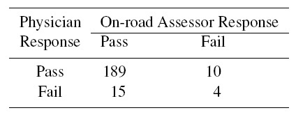
- Is there a bias between physicians and on-road assessors in terms of fitness-to-drive decisions?
- Determine the sample κ statistic and interpret it.
- Determine 95% lower confidence bounds for the population kappa coefficient using (i) the basic formula based on normal approximation (ii) bootstrapping methodology.
- This exercise introduces other parameters discussed in the agreement literature for categorical ratings (e.g., Byrt et al., 1993). In a 2 × 2 agreement problem, (i) | p12 − p21 | is called the bias index (BI), (ii) | p11 − p22 | is called the prevalence index (PI) (iii) 2(p11 + p22) − 1 ≡ 2 θ − 1 is called the prevalence adjusted, bias adjusted kappa index (PABAK).
- Find the range for each of the above indices.
- Establish the following relationship between κ and them:
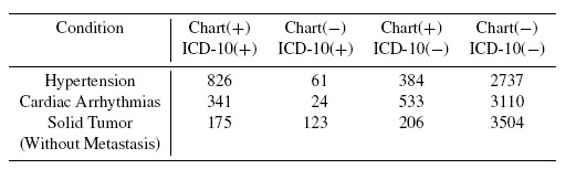
- International Classification of Diseases, Tenth Revision (ICD-10), developed by the World Health Organization, contains codes and classifications for patient medical conditions and are followed all over the world. Chen et al. (2009) have measured agreement on 32 conditions between data from an ICD-10 administrative database and from chart reviews of 4008 discharges from four hospitals in Alberta, Canada. The data presented in Table 12.6 on three conditions is extracted from their Table 2.
- Compute the sample estimates of κ, BI, PI, and PABAK for each of the three medical conditions.
- In each case, compare the estimates of κ and PABAK and comment on the degree of agreement between the discharge charts and the corresponding ICD-10 database.
Table 12.6 Frequencies of observed classifications for disease classification data for Exercise 12.15.
- Consider the two-way random effects model given in (12.34) and assume normality. Define the following random variables:
- Write down the ANOVA table that includes the sources of variation (Between Subjects, Between Raters, Error, and Total), associated degrees of freedom, and sum of squares in terms of the above averages. Denote the mean sum of squares by SMS for subjects, RMS for raters, and EMS for the error.
- Determine the expected values for SMS, RMS, and EMS.
- Using method of moments, determine the estimates of the variance components
 .
. Let
 C be the estimate of ρC defined in (12.35). Show that
Define F = RMS/EMS and
Note that ν is random, data dependent, and may be a non-integer.
Let F0 denote 95 th percentile of an F distribution with degrees of freedom n − 1 and ν. Show that an approximate 95% lower confidence bound for ρC is given by
[Hint: See the discussion in Fleiss and Shrout, 1978.]
- Fleiss (1971) presents an example where each of 30 patients were evaluated by six psychiatrists, and different psychiatrists participated in the evaluation of distinct subjects. Each rater classified a patient into one of five mutually exclusive categories: depression, personality disorder, schizophrenia, neurosis, and other. The data are summarized in Table 12.7.
Table 12.7 Frequencies of observed evaluations of six psychiatrists for 30 patients for Exercise 12.17.
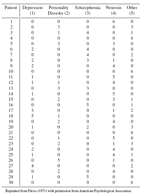
- Write down the two-way random effects model given in (12.34) for these data.
- Assuming the model given above in (a), find the intraclass correlation (
 C) representing the association between two ratings of the same subject using standard ANOVA methods.
 For the multi-rater, multi-category rating setup, Fleiss (1971) introduced sample overall κ coefficient with the following formula:
Here n is the number of subjects; J is the number of raters, each rating every subject into one of c categories; and mij is the number of raters out of J that are classifying ith subject into jth category. Further,
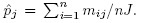 Determine
  O for the data given in Table 12.17 representing the mij for the 30 patients.
- Compare the intraclass correlation C obtained using the ANOVA model, and O.
- Obtain a 95% lower confidence bound for ρC using the methodology described in Exercise 12.16.
-
- Establish that var(C) for the model given in (12.34) can be approximated by the expression in (12.36). [Hint: Use bivariate Taylor series approximation for the variance of a ratio of random variables.]
- Give an estimate of the standard error of C for the data given in Exercise 12.17 using this formula.
- Establish that var(
-
- Establish the expression given in (12.45) for the probit generalized linear mixed-effects model.
- Show that the expression for κM simplifies to the one given in (12.46).
- Develop an expression for the Cohen’s kappa coefficient for a logit generalized linear mixed-effects model for binary data. (See Nelson and Edwards, 2008.)
- The sample size formula (12.28) can also be used in conjunction with testing agreement hypotheses (1.13) based on common agreement measures for continuous data. Further simplification of the formula is possible if
 , which equals
  /n in the formula, can be replaced by its upper bound. For z -transformed CCC (see, page 80, Section 3.3.3), an approximate upper bound for the variance estimate is 1 /(n − 2) (Lin et al., 2011, Section 4.2).
Show that using this bound in (12.28) yields the following sample size formula for inference on CCC:
where tanh−1(CCC0) and tanh−1(CCC1), respectively, represent the null and alternative values of Fisher’s z-transformation of CCC.
- Use the above formula to compute the sample size necessary for a 5% level test of hypotheses (1.13) based on CCC to have 80% power when CCC0 = 0.90 represents the boundary for insufficient agreement and CCC1 = 0.98 is the anticipated high level of agreement.