CHAPTER 5
REPEATED MEASUREMENTS DATA
5.1 PREVIEW
This chapter presents a methodology for the analysis of studies comparing two methods wherein both take multiple measurements on each subject. It focuses on two types of repeated measurements data—unlinked and linked. The usual steps in analysis consist of displaying data, modeling of data via a mixed-effects model, and associated evaluation of similarity and agreement. With repeated measurements, one can also evaluate repeatability of each method, which amounts to self-agreement. The methodology is illustrated with two case studies.
5.2 INTRODUCTION
Let Yijk denote the kth repeated measurement of the jth method on the ith subject. The data consist of Yijk, k = 1,...,mij, j = 1, 2, i = 1,...,n. Here n is the number of subjects in the study and mij is the number of measurements of method j on subject i. It is assumed that mij ≥ 2. Let Mi = mi1 + mi2 and ![]() , respectively, denote the total number of measurements on the ith subject and in the entire dataset. When mi1 = mi2, we will use mi to denote the common value. Moreover, when the mi are equal, the common value will be denoted by m. The design is balanced if each method has the same number m of measurements on every subject, otherwise it is unbalanced. Measurements on the same subject are dependent, whereas those from different subjects are assumed to be independent. It is necessary to appropriately model the dependence among the repeated measurements on the same subject to get accurate estimates.
, respectively, denote the total number of measurements on the ith subject and in the entire dataset. When mi1 = mi2, we will use mi to denote the common value. Moreover, when the mi are equal, the common value will be denoted by m. The design is balanced if each method has the same number m of measurements on every subject, otherwise it is unbalanced. Measurements on the same subject are dependent, whereas those from different subjects are assumed to be independent. It is necessary to appropriately model the dependence among the repeated measurements on the same subject to get accurate estimates.
5.2.1 Types of Data
Often “repeated measurements data” is used as a catch-all term to refer to any type of data wherein multiple measurements are available on each subject. Here we distinguish between three types of repeated measurements, viz., unlinked, linked, and longitudinal. This distinction is important as it affects how the data are modeled. These data types are described next.
The repeated measurements on a subject are unlinked (or unpaired) if the measurements from the two methods are obtained separately, and a method’s multiple measurements on a subject are independent replications of the same underlying measurement. By replication, we mean repeating a measurement under identical conditions, ensuring that the true value of the subject remains unchanged during the measurement period. The methods need not have the same number of measurements on a subject. Essentially a method’s unlinked repeated measurements are identically distributed. They may arise, for example, when the multiple measurements are taken in quick succession or when a subject’s homogeneous specimen is subsampled to get the multiple measurements. The assumption of independence holds if the multiple measurements are taken without influencing each other. The kiwi data to be introduced in Section 5.2.3 is an example of unlinked repeated measurements data.
The repeated measurements on a subject are linked (or paired) when the measurements from the two methods are made together in pairs as (Yi1k, Yi2k), k = 1,...,mi. The measurements in each pair are linked by a common condition k, which we call “time.” Often this time factor is an actual measurement occasion. Obviously, the contribution of each subject to the data consists of two paired trajectories over time, one for each method. Unlike the unlinked case, the methods necessarily have an equal number of measurements on a subject. This means mi1 = mi2 = mi in our notation, but mi may vary from subject to subject. In addition, the true value need not remain constant over time, and usually it does not. For this reason, we refrain from calling the repeated pairs as replications. Naturally, the order in which the linked measurements are made matters. However, it is assumed that there is no systematic effect of time on the paired trajectories beyond the dependence induced in them by the common measurement time. Linked repeated measurements may arise when the quantity being measured itself keeps changing, for example, blood pressure or heart rate, and it is the instantaneous measurement that is of interest. The oximetry data in Section 5.2.3 is an example of such data.
The repeated measurements on a subject are longitudinal when the measurements from both methods are made over a period of time, and unlike the linked case, there is a systematic fixed effect of time or a time-dependent covariate on the measurements. Thus, the contribution of each subject consists of two trajectories over time, but these may or may not be paired over the measurement times. The true value of the subject necessarily changes, making the time of measurement important. The time may be a discrete quantity with a small number of values (e.g., before and after an intervention or a visit number), or it may be a continuous quantity (e.g., age of subject at the time of measurement). Unlike linked and unlinked data, longitudinal data necessitates modeling the measurement trajectories as functions of time, warranting a special treatment of its own. Therefore, this chapter only considers unlinked and linked data; longitudinal data is the subject of Chapter 9.
5.2.2 Individual versus Average Measurement
The analysis of repeated measurements data involves a decision as to whether a subject’s individual measurements or their average value should be the object of analysis. This issue is generally relevant only for the unlinked data because they consist of replications of the same underlying measurements. Linked and longitudinal data are usually not structured like this; but when they do consist of such replications, this issue would be relevant there as well.
The decision about the object of analysis is informed by how the methods are used in common practice. If it is customary to replicate measurements but use their average value, obviously the individual measurements should be averaged, and the methodology of Chapter 4 should be applied to the paired averages. If, however, we want to use the multiple measurements individually, which is usually the case in practice, the methodology of this chapter is appropriate. The measurements in this case should not be averaged prior to analysis because doing so will make the methods seem more precise, and hence the methods will exhibit more agreement than observed in practice. Even though a single measurement may be the standard procedure, it is a good idea to replicate the measurements anyway because this allows reliable estimation of precisions of the methods.
5.2.3 Example Datasets
We now introduce two datasets that will be used as illustrative examples in this chapter.
5.2.3.1 Kiwi Eggshell Data
These data were collected in a study of thickness of avian eggshell, a quantity of particular interest to ecologists because it has a direct bearing on the strength of the eggshell. The thickness of the shell of an egg is not uniform; the shell is thinnest and most uniform at the equator, and thickest at the two poles. The study compared two methods for measuring eggshell thickness. One is the usual caliper type micrometer (method 1) and the other is a scanning electron microscope (method 2). A micrometer is portable, cost-effective, and can be easily used anywhere. However, its use may be unsuitable if the fragility of eggshells is of concern. This may happen, for instance, if the eggshells come from museum collections. The microscope offers a less invasive alternative than the micrometer, but it has disadvantages of its own. They include its cost, time, and electricity requirement, restricting its usage, for example, in remote locations.
In the study, the thickness of eggshell fragments from the equatorial region of eggs of 16 North Island brown kiwis (Apteryx mantelli), which are small flightless birds native to New Zealand, was measured (in μm) at three randomly selected locations using both methods. The three locations for each method were different. Each eggshell fragment came from a different egg and the same individual took all the measurements. The design of this study is balanced. Repeated measurements here are unlinked because the two methods measure at different locations and the true value at these locations are considered same due to uniformity of thickness in the equatorial region.
5.2.3.2 Oximetry Data
The oximetry data come from a study conducted in infants at Royal Children’s Hospital in Melbourne, Australia. It compared two methods for measuring percent oxygen saturation in blood, namely, pulse oximetry (method 1) and CO-oximetry (method 2). The former is a noninvasive method that indirectly measures oxygen saturation using a sensor placed on a thin body part, for example, fingertip. The latter uses a blood specimen to directly measure oxygen saturation. The study involved 61 infants. Among them, 56 were measured on three occasions, four were measured on two occasions, and one was measured on only one occasion. Thus, the study design was unbalanced. The repeated measurements here are linked because they are paired over the measurement times.
5.3 DISPLAYING DATA
5.3.1 Basic Plots
Basic graphical tools for displaying paired data wherein each subject contributes a pair of measurements are the trellis plot, the scatterplot, and the Bland-Altman plot. These plots need to be adapted to display repeated measurements data. A key consideration is that, in addition to displaying the usual data features, they should also allow us the ability to effectively examine the within-and between-subject variations—a key motivation for collecting repeated measurements in the first place.
5.3.1.1 Trellis Plot
By design, the vertical axis of this plot is divided into rows and each row displays all data on a subject using method-specific symbols. Thus, for unlinked as well as linked data, each row will now have multiple measurements per method instead of a single measurement it had for the paired data. Figures 5.1 and 5.2 show trellis plots of kiwi and oximetry data, respectively. The first data are unlinked, whereas the second data are linked. A trellis plot, in addition to allowing examination of the overlap of the data produced by the two methods and comparison of their biases, makes it easy to see a number of data features of interest. It shows how the within-subject variations of the two methods compare, whether they change with magnitude of measurement or not, and how they relate to the between-subject variation. It also shows whether there is any subject × method interaction. It, however, does not preserve information about the pairing that is inherent in the linked data. Detailed interpretation of the plots is postponed until Section 5.7, where the case studies are presented.
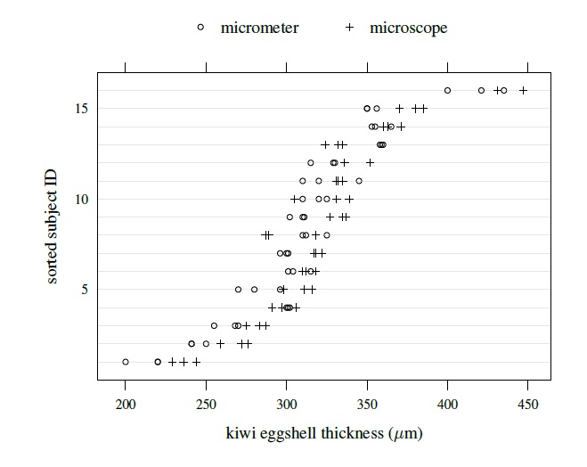
Figure 5.1 Trellis plot of kiwi data.
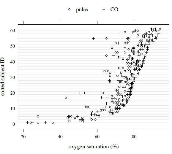
Figure 5.2 Trellis plot of oximetry data.
5.3.1.2 Scatterplot and Bland-Altman Plot
Ordinarily, these plots display one measurement pair per subject and the data from different subjects are independent, justifying using the same plotting symbol for each subject. With linked repeated measurements, each subject contributes multiple dependent measurement pairs. This dependence structure can be shown in the plot by using a subject-specific plotting symbol. Otherwise that information will be lost and the plots will often give a wrong impression of the dependence structure. A numerical subject ID is a natural choice for the subject-specific plotting symbol. In practice, however, it may be hard to distinguish between the subjects if a large number of them cluster together. This happens in the top panel of Figure 5.3, where scatterplot and Bland-Altman plot are shown for the oximetry data. Another possibility is to use the same symbol for all data but connect the points coming from the same subject by a line. This version is presented in the bottom panel of Figure 5.3. Both versions essentially convey the same information, and they do not show the within-subject variation as clearly as the trellis plot.
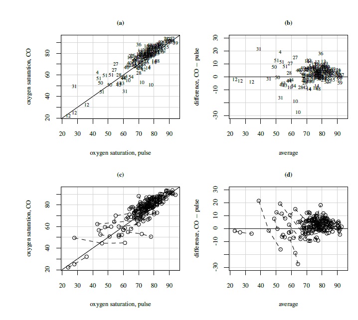
Figure 5.3 Plots for oximetry data. Top panel (left to right): Scatterplot with line of equality and Bland-Altman plot with zero line, with subject ID (1 to 61) as plotting symbol. Bottom panel (left to right): Same as top panel but with a common plotting symbol and points from the same subject joined by a broken line.
The unlinked data do not have natural pairings of a subject’s multiple measurements from the two methods. However, to display them in a scatterplot or a Bland-Altman plot, we need to identify one pair per subject. There are two ways to form such pairs. One is to randomly select one measurement per method from the available measurements of a subject. The justification for this is that the unlinked repeated measurements data are assumed to exhibit a distributional symmetry. Randomly choosing only one measurement per method to display in the plot preserves the essential information and is supported by this symmetry. The other alternative is to compute method-specific averages for each subject. But the averaging will make the methods appear more precise and show better agreement than shown by individual pairs, especially if the within-subject variation is large. In either case, the resulting plots may look sparse if n is small. In addition, their construction masks the within-subject variation. Figure 5.4 displays both versions of the scatterplot and the Bland-Altman plot for the kiwi data. The effect of averaging is more visible in the Bland-Altman plot in the form of reduced range for the difference on the vertical axis.

Figure 5.4 Plots for kiwi eggshell thickness data. Top panel (left to right): Scatterplot with line of equality and Bland-Altman plot with zero line based on 16 randomly formed measurement pairs. Bottom panel (left to right): Same as top panel but based on 16 average measurements.
For linked data we have not considered plots based on either single measurements or averages. This is because the true values therein may change over the measurement period. Taking only a single measurement or an average will result in substantial loss of information, making this an inadequate choice. We also see that none of the modified versions of the scatterplot shows the within-subject variation as clearly as a trellis plot. Nonetheless, the scatterplots as well as the Bland-Altman plots are useful because they provide complementary information, just like in the case of paired data.
5.3.2 Interaction Plots
Repeated measurements data also allow us to incorporate certain interactions in the analysis that may be present in the data (see Section 5.4). The two interactions of particular interest are subject × method interaction, relevant for both unlinked and linked data, and subject × time interaction, relevant only for the latter. While it may be possible to see evidence of their presence in the aforementioned plots, it is formally explored through interaction plots. To describe them, let
be the average over the repeated measurements for method j, and
be the average over the methods at time k. The latter is relevant only for linked data, in which case mij = mi.
For subject × method interaction, we can plot average ![]() ij· against method j (j = 1, 2), separately for each subject i, with points for each subject connected by a line. Similarly, for subject × time interaction, we can plot average
ij· against method j (j = 1, 2), separately for each subject i, with points for each subject connected by a line. Similarly, for subject × time interaction, we can plot average ![]() i.k against time k (k = 1,...,mi), separately for each subject i, with points for each subject connected by lines. Both these interaction plots consist of n connected lines, one for each subject. In either case, there is evidence of interaction if the lines are not parallel.
i.k against time k (k = 1,...,mi), separately for each subject i, with points for each subject connected by lines. Both these interaction plots consist of n connected lines, one for each subject. In either case, there is evidence of interaction if the lines are not parallel.
Figure 5.5 displays a subject × method interaction plot for kiwi data. Figure 5.6 displays two interaction plots for oximetry data—one for subject × method interaction and the other for subject × time interaction. All show clear evidence of interaction.
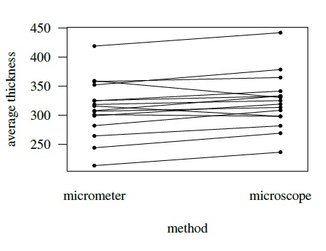
Figure 5.5 Interaction plot for kiwi data depicting subject × method interaction. Lines join points from the same subject.
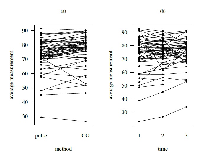
Figure 5.6 Interaction plots for oximetry data depicting subject × method interaction (left panel) and subject × time interaction (right panel). Lines join points from the same subject.
5.4 MODELING OF DATA
Models for repeated measurements data depend on whether they are unlinked or linked. We consider these scenarios in turn.
5.4.1 Unlinked Data
Here the data consist of Yijk, k = 1,...,mij, j = 1, 2, i = 1,...,n, where a method’s multiple measurements on a subject are replications of the same underlying measurement. The two methods are replicated separately, implying that their measurements on a subject are dependent but not paired. The measurements from different subjects are assumed to be independent, as always. To model these data, we consider the basic mixed-effects model (4.1) for paired measurements data and add to it a random subject × method interaction term bij. Thus, the model can be written as
k = 1,...,mij , j = 1, 2, i = 1,...,n. As in (4.1), the methods are assumed to have the same scale. Moreover, bi remains the true unobservable measurement of the ith subject, β0 remains the difference in the fixed biases of the methods, and eijk are random errors.
We now consider interpreting the interaction term bij. One way is to think of it as the effect of method j on subject i. In other words, these interactions are subject-specific biases of the methods. For another interpretation, recall that bi and β0 + bi are, respectively, the true values of methods 1 and 2 for subject i (Section 1.6). However, their error-free values under (5.1) are bi + bi1 and β0 + bi + bi2, respectively. The true values and the error-free values differ by bij in the case of method j. This suggests that bij can be interpreted as an error in equation of method j. The equation error bij is different from the random error eijk. The former is a characteristic of the method-subject combination that remains stable during the measurement period. The latter fluctuates from measurement to measurement within a subject. While we call bij as an interaction in keeping with the terminology in mixed-effects modeling, it is indeed called an equation error in measurement error modeling. It is also known as a matrix effect in analytical chemistry. A matrix refers to a substance that dissolves a chemical of interest. It plays the role of a subject in our terminology.
To complete the specification of the model (5.1), we make the usual normality and independence assumptions for the random quantities:
- bi follow independent
 distributions,
 - bij follow independent N1(0, ψ2) distributions,
- eijk follow independent
 distributions, and
 - bi, bij, and eijk are mutually independent.
The random errors have method-specific variances, but the interaction effects have a common variance for the two methods. It is also possible to let the variance of the interaction term depend on the method. Although the resulting model is identifiable, reliable estimation of both the variances becomes an issue. A similar situation arose in Chapter 4 for estimation of two error variances with paired data. Therefore, we assume a common variance for the interactions for the time being. This assumption is relaxed in Chapter 7, where more than two methods are compared.
In model (5.1), the effect of a subject manifests on the measurements through three independent quantities, namely, bi, bi1, and bi2. Upon averaging out the subject effects we see that the vectors of Mi = mi1 + mi2 measurements on subject i = 1,...,n follow independent Mi-variate normal distributions with means (Exercise 5.1)
and variances
Further,
is the common covariance between two replications of the same method, and
is the common covariance between any two measurements from different methods on the same subject. The first covariance involves two variance components because a method’s replications on a subject i shares two random effects—the true measurement bi and the interaction effect bij. The second covariance involves only one variance component because the measurements from different methods share only the bi. The model (5.1) has a total of six unknown parameters, namely, ![]() .
.
Even though we have replicated measurements, our ultimate interest is in evaluating how close a measurement from one method on a subject is to a measurement from the other method on the same subject. This evaluation requires examination of measures of similarity and agreement derived from the distribution of (Y1, Y2), a pair of measurements by the two methods on a randomly selected subject from the population (Section 1.7). The assumed model (5.1) induces a distribution for (Y1, Y2). Drop the subscripts i and k in (5.1) to obtain the companion model for (Y1, Y2) as
where b, bj , and ej are identically distributed as bi, bij , and eijk, respectively. Proceeding as before gives (Exercise 5.2)
It follows that
Notice that taking the difference eliminates the effect of true value bi but the effect of interaction bij remains. The measures of similarity and agreement based on these distributions are derived in Section 5.5.
5.4.2 Linked Data
The data in the linked case consist of paired measurements (Yi1k, Yi2k) over time k = 1,...,mi. These data are also modeled as (5.1) except that we add a term ![]() representing the random effect of the common time k on the measurements. This random effect links the measurements at the time k. The model becomes
representing the random effect of the common time k on the measurements. This random effect links the measurements at the time k. The model becomes
The ![]() follow independent
follow independent ![]() distributions and they are mutually independent of bi, bij , and eijk, which continue to follow the assumptions made for model (5.1). The distribution of
distributions and they are mutually independent of bi, bij , and eijk, which continue to follow the assumptions made for model (5.1). The distribution of ![]() does not depend on either method or time.
does not depend on either method or time.
The effect ![]() can also be interpreted as a subject × time interaction. In other words,
can also be interpreted as a subject × time interaction. In other words, ![]() is a subject-specific bias that gets introduced in the measurements at time k. It is instructive to contrast the interactions bij and
is a subject-specific bias that gets introduced in the measurements at time k. It is instructive to contrast the interactions bij and ![]() . The former is a characteristic that depends on method but remains stable over time. The latter is a characteristic that does not depend on method and captures the change in the true value of the ith subject over time. Both effects, however, vary from subject to subject and these variations are modeled via normal distributions.
. The former is a characteristic that depends on method but remains stable over time. The latter is a characteristic that does not depend on method and captures the change in the true value of the ith subject over time. Both effects, however, vary from subject to subject and these variations are modeled via normal distributions.
The effect of a subject on the measurements now manifests through independent random variables bi, bij, and ![]() . The distributions of vectors of Mi (= 2mi) measurements on subject i = 1,...,n are independent Mi-variate normals with means (Exercise 5.3)
. The distributions of vectors of Mi (= 2mi) measurements on subject i = 1,...,n are independent Mi-variate normals with means (Exercise 5.3)
and variances
In addition, there are three distinct covariances. The first is the covariance between two measurements of the same method,
This covariance is attributed to two random effects—bi and bij—that the measurements have in common. The second is the covariance between measurements from different methods taken at the same time,
This covariance is also attributed to two random effects—bi and ![]() —that the measurements share. Notice how the random effect of time k induces covariance in the two measurements taken at the particular time point. The last is the common covariance between measurements from different methods taken at different times,
—that the measurements share. Notice how the random effect of time k induces covariance in the two measurements taken at the particular time point. The last is the common covariance between measurements from different methods taken at different times,
This covariance is attributed to the only random effect bi that the measurements share. The model (5.9) has seven unknown parameters, namely, ![]() .
.
Recall from Section 5.2.1 that even though we have linked measurements over a period of time, we are interested in comparing methods with respect to their measurements on a subject at any particular instant. This means we again need to find the distribution of a single measurement pair (Y1, Y2) induced by the assumed model (5.9). We now proceed as in the unlinked case to obtain this distribution. Dropping the subscripts i and k in (5.9), the companion model for (Y1, Y2) can be written as
where b, bj, b*, and ej are identically distributed as bi, bij , ![]() , and eijk, respectively. It follows that (Exercise 5.4)
, and eijk, respectively. It follows that (Exercise 5.4)

This implies
There are two noteworthy features of this distribution. First, it does not involve any effect of time. Second, it is identical to the one obtained in (5.8) for the unlinked case even though the two data models are different. This happens because the effect of the true value at a given time is eliminated upon differencing, and only the effects of random errors and subject × method interactions remain in the difference. We return to these distributions in Section 5.5 to obtain measures of similarity and agreement.
5.4.3 Model Fitting and Evaluation
The models for both unlinked and linked data can be fit by the ML method using a statistical software that fits mixed-effects models (see Section 5.9 for some technical details). For (5.1), we will have the ML estimates ![]() of the model parameters, predicted values
of the model parameters, predicted values ![]() of the random effects, and the fitted values
of the random effects, and the fitted values
Analogously, for (5.9), we will have the ML estimates ![]() of the model parameters, predicted values
of the model parameters, predicted values ![]() of the random effects, and the fitted values
of the random effects, and the fitted values
In both cases, the residuals are ![]() and
and ![]() are their standardized counterparts.
are their standardized counterparts.
Both models involve a number of assumptions. These can be verified by the usual model diagnostics. In particular, one can examine the Bland-Altman plot for the equal scales assumption, the plot of standardized residuals against fitted values for the homoscedasticity and the zero mean assumptions for random errors, and Q-Q plots of standardized residuals and predicted random effects for the normality assumptions. It is often a good idea to examine residual and Q-Q plots for the two methods separately to reveal any method-specific structures that may be present.
Moreover, as in Chapter 4, we do not normally look for submodels of the original models (5.1) and (5.9) with the intent of obtaining a more parsimonious description of data. The original models are basic to begin with, and we prefer to use measures of similarity and agreement based on these models to quantify any differences in the method-specific parameters.
It often happens that not all variance components in model (5.1) or (5.9) are estimated reliably with the data available. This is evident when at least one of the estimated variance components is near zero or has an unusually large standard error. In this case, we may proceed by either dropping the interaction term bij from the model, or adopting a model where the bi term is dropped and (bi1,bi2) are assumed to be i.i.d. draws from a bivariate normal distribution with mean vector (β1, β2) and an unstructured covariance matrix (see also Exercise 7.12). The methodology of the next two sections can be easily modified to accommodate these changes to the model.
5.5 EVALUATION OF SIMILARITY AND AGREEMENT
Evaluation of similarity calls for examining differences in marginal distributions of Y1 and Y2 through estimates and two-sided confidence intervals (Section 1.7). The distributions of Y1 and Y2 are given in (5.7) for unlinked and in (5.16) for linked data. The similarity measures of interest include the intercept β0, representing the difference in the fixed biases of the methods, and the precision ratio ![]() This λ compares only the random errors of the two methods; it ignores their equation errors, that is, the subject × method interactions. They can also be included in the comparison by replacing
This λ compares only the random errors of the two methods; it ignores their equation errors, that is, the subject × method interactions. They can also be included in the comparison by replacing ![]() with
with ![]() to get the following modification of λ:
to get the following modification of λ:
Often, however, both λ and λ1 lead to the same conclusion regarding similarity.
To evaluate agreement, one has to examine estimates and one-sided confidence bounds for measures of agreement based upon the joint distribution of (Y1, Y2). The two agreement measures of specific interest are CCC and TDI. From its definition in (2.6), CCC for unlinked data can be written as
and CCC for linked data is
The TDI measure is based on the difference D. We saw from (5.8) and (5.17) that D has the same distribution for unlinked as well as linked data. Therefore, TDI has the same expression in both cases. From its definition in (2.29),
As before, the ML estimators of measures of similarity and agreement are obtained by replacing the unknown parameters in their expressions by their respective ML estimators. Furthermore, the large-sample theory is used to compute standard errors and confidence bounds and intervals (Section 5.9). One can also use the distribution of D to compute the 95% limits of agreement in both unlinked and linked cases as
5.6 EVALUATION OF REPEATABILITY
Repeatability of a method refers to its agreement with itself. It is important to evaluate this intra-method agreement because, if a method does not agree well with itself, it cannot be expected to agree well with another method. The evaluation of a method’s repeatability is essentially an evaluation of its error variation. The repeated measurements data make this evaluation possible.
Repeatability measures are distinct from the measures of agreement that quantify how much the two methods agree, and the measures of similarity that quantify differences in marginal distributions of the methods. The extent of intra-method agreement that a repeatability measure quantifies serves as a benchmark for the extent of inter-method agreement quantified by an agreement measure.
From the viewpoint of benchmarking, an attractive way to measure intra-method agreement is to adapt the measures of agreement that have been developed for measuring inter-method agreement. The inference on them proceeds exactly in the same manner as the agreement measures. Such repeatability measures are derived next.
5.6.1 Unlinked Data
Here the repeated measurements are replications of the same underlying measurement. We have been using (Y1, Y2) to denote measurements by the two methods on a randomly selected subject from the population. Now let ![]() be a replication of Y1 and
be a replication of Y1 and ![]() be a replication of Y2 on the same subject. By definition, Yj and
be a replication of Y2 on the same subject. By definition, Yj and ![]() have the same marginal distribution. To find their joint distribution, recall that the assumed data model (5.1) induces a companion model (5.6) for (Y1, Y2). Similarly, it also induces a companion model for (
have the same marginal distribution. To find their joint distribution, recall that the assumed data model (5.1) induces a companion model (5.6) for (Y1, Y2). Similarly, it also induces a companion model for (![]() ,
, ![]() ) as:
) as:
where ![]() and
and ![]() are independent copies of e1 and e2, respectively, both of which are defined in (5.6). It follows from the two companion models (5.6) and (5.23) that (Exercise 5.2)
are independent copies of e1 and e2, respectively, both of which are defined in (5.6). It follows from the two companion models (5.6) and (5.23) that (Exercise 5.2)
and
Define Dj = Yj ‒ ![]() as the difference in two replications of method j. From (5.24) and (5.25), we have
as the difference in two replications of method j. From (5.24) and (5.25), we have
We know that an agreement measure is a function of parameters of the bivariate distribution of (Y1, Y2). Taking the same function of parameters but of the bivariate distribution of (Yj , ![]() ) yields a measure of repeatability (or intra-method agreement) of method j. This approach would produce an analog of any agreement measure for measuring self-agreement. For example, the repeatability versions of CCC and TDI are (Exercise 5.2)
) yields a measure of repeatability (or intra-method agreement) of method j. This approach would produce an analog of any agreement measure for measuring self-agreement. For example, the repeatability versions of CCC and TDI are (Exercise 5.2)
Notice that CCCj is simply the intraclass correlation between Yj and ![]() as the two measurements have identical means and variances. A comparison with (1.4) shows that CCCj is in fact the reliability of method j because it can be interpreted as the proportion of total variation not explained by the within-subject errors. Notice also that TDIj is just a constant multiple of the error variation of method j. These expressions essentially reinforce that a repeatability measure is a measure of a method’s error variation. The distribution of Dj in (5.26) can also be used to get the repeatability analog of the 95% limits of agreement for method j as
as the two measurements have identical means and variances. A comparison with (1.4) shows that CCCj is in fact the reliability of method j because it can be interpreted as the proportion of total variation not explained by the within-subject errors. Notice also that TDIj is just a constant multiple of the error variation of method j. These expressions essentially reinforce that a repeatability measure is a measure of a method’s error variation. The distribution of Dj in (5.26) can also be used to get the repeatability analog of the 95% limits of agreement for method j as
5.6.2 Linked Data
Paralleling the above development, let (![]() ,
, ![]() ) be another pair of measurements taken by the two methods on the same subject that gives (Y1, Y2) but at another time. We do not call (
) be another pair of measurements taken by the two methods on the same subject that gives (Y1, Y2) but at another time. We do not call (![]() ,
, ![]() ) a replication of (Y1, Y2) as the underlying true value may not be the same.
) a replication of (Y1, Y2) as the underlying true value may not be the same.
The companion model for (Y1, Y2) induced by the data model (5.9) is given by (5.15). The corresponding companion model for (![]() ,
, ![]() ) is
) is
where b**, ![]() , and
, and ![]() are independent copies of b*, e1, and e2, respectively, all defined in (5.15). As before, it can be seen from (5.15) and (5.29) that (Exercise 5.4)
are independent copies of b*, e1, and e2, respectively, all defined in (5.15). As before, it can be seen from (5.15) and (5.29) that (Exercise 5.4)

and

Moreover,
Notice the effect of time on Dj in the form of the variance component ![]() . To see where this comes from, use (5.15) and (5.29) to write
. To see where this comes from, use (5.15) and (5.29) to write
making it explicit that Dj has two sources of variation—the difference in effects of times as well as errors. This contrasts with the unlinked case where the effect of time is absent.
As before, versions of CCC and TDI for measuring repeatability can be deduced from (5.30), (5.31), and (5.32) as (Exercise 5.4)
Although this CCCj is also the intraclass correlation between Yj and ![]() , it is not a reliability measure in the strict sense of (1.4) because it does not represent the proportion of total variation not explained by the errors. This interpretation is possible if we think of the effect of time as a part of the error. It also allows TDIj to be interpreted as a constant times the error variation of method j, just like the unlinked case. Moreover, the 95% limits of intra-method agreement for method j using (5.32) are:
, it is not a reliability measure in the strict sense of (1.4) because it does not represent the proportion of total variation not explained by the errors. This interpretation is possible if we think of the effect of time as a part of the error. It also allows TDIj to be interpreted as a constant times the error variation of method j, just like the unlinked case. Moreover, the 95% limits of intra-method agreement for method j using (5.32) are:
It is instructive to ask: “Can a method agree more with another method than with itself?” Intuitively, we expect the answer to be no in general. This is indeed the case for unlinked data, but the linked data are a different matter altogether; see, for example, the analysis of the oximetry data in the next section and also Exercise 5.5.
5.7 CASE STUDIES
5.7.1 Kiwi Data
The kiwi data, introduced in Section 5.2.3, consist of measurements of thickness (in μm) of n = 16 kiwi eggshells from a micrometer (method 1) and a scanning electron microscope (method 2). The data are unlinked and we have a balanced design with m = 3 replications. We have already seen a number of plots of these data—a trellis plot in Figure 5.1, scatterplots and Bland-Altman plots of 16 randomly selected and of average over replications in Figure 5.4, and a subject × method interaction plot in Figure 5.5. The trellis plot clearly shows that microscope measurements are larger than micrometer for almost all subjects, indicating a difference in fixed biases of the methods. The difference between the methods does not seem to be constant over the subjects, implying a subject × method interaction, which is confirmed by the crossings of the lines in the interaction plot. The trellis plot also shows that the within-subject variation of both methods are comparable and are small in comparison with the between-subject variation. The data appear homoscedastic because the within-subject variation does not seem to vary much over the measurement range. The scatterplots of both individual and average measurements show high correlation between the methods. The microscope’s tendency to produce higher readings is confirmed by both sets of scatterplots and Bland-Altman plots. The latter plots do not exhibit any trend, implying that the methods can be assumed to have equal scales. This assumption is needed for modeling of data using the mixed-effects model (5.1).
The next step is to fit this model. The resulting residual plot in Figure 5.7 is centered at zero and does not exhibit any pattern. The normality assumption for errors and random effects is checked in Exercise 5.6. On the whole, the model appears to fit reasonably well.
Table 5.1 presents ML estimates of model parameters and their standard errors. Both methods have considerable random error variation ![]() . Their magnitudes are comparable to that of the subject × method interaction
. Their magnitudes are comparable to that of the subject × method interaction ![]() . Substitution of the estimates in (5.7) and (5.8) gives the fitted distributions of (Y1, Y2) and D = Y2 ‒ Y1 as
. Substitution of the estimates in (5.7) and (5.8) gives the fitted distributions of (Y1, Y2) and D = Y2 ‒ Y1 as

On average, a measurement of thickness of a specimen from the microscope exceeds that from the micrometer by 11.35. The methods have comparable variances and their correlation is 0.92. The differences in measurements have a standard deviation of ![]() . Both the errors and the interactions contribute about equally to the variation in D. From (5.22), the 95% limits of agreement between the methods are 11.35 ± 1.96 * 18.9 = (‒26, 48).
. Both the errors and the interactions contribute about equally to the variation in D. From (5.22), the 95% limits of agreement between the methods are 11.35 ± 1.96 * 18.9 = (‒26, 48).
Substitution of the parameter estimates in (5.24) and (5.25) gives the fitted distributions of (Y1, ![]() ) and (Y2,
) and (Y2, ![]() ). The marginal distribution of
). The marginal distribution of ![]() is the same as that of Yj and their correlation is 0.96 for both methods. From (5.26), the fitted distributions of the intra-method differences Dj are:
is the same as that of Yj and their correlation is 0.96 for both methods. From (5.26), the fitted distributions of the intra-method differences Dj are:
These have zero means by definition, and their standard deviations are about 13. Thus, from (5.28), the 95% limits of intra-method agreement are ![]() for micrometer, and
for micrometer, and ![]() for microscope.
for microscope.
Table 5.1 provides estimates and 95% confidence intervals for β0 and λ for similarity evaluation. The interval for β0 is (4, 19). It confirms larger fixed bias of microscope compared to micrometer as the lower limit is above zero. The interval for λ is (0.5, 2). Although the estimated λ of 1.1 shows slightly better precision for microscope, the confidence interval allows us to conclude that the methods have practically the same precision.
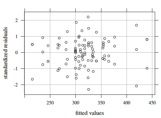
Figure 5.7 Residual plot for kiwi data.
An identical conclusion follows from the 95% confidence interval (0.7, 1.4) for λ1 (not presented in the table). This modification of λ, defined in (5.18), incorporates the variation of subject × method interactions in the comparison in addition to that of the errors.
Table 5.1 also provides estimates and one-sided 95% confidence bounds for intra-method versions of CCC and TDI (0.90) for evaluating repeatability. Clearly, the methods have similar repeatability on both measures. This finding, however, is not surprising since repeatability is essentially a measure of error variation and we just saw that the methods have similar precisions. More revealing are the actual values of the estimates and the bounds. The CCC estimates, which also represent the estimated reliabilities, are 0.96. This essentially shows that the error variations are a small portion of the total variation in the measurements. The TDI bounds of 26 imply that 90% of the time the difference between two replicate measurements from the same method on the same eggshell falls within ±26. This bound of 26 is about 8% of ![]() . The measurements themselves range between 200 and 450. This extent of repeatability was acceptable to the ecologists conducting the study.
. The measurements themselves range between 200 and 450. This extent of repeatability was acceptable to the ecologists conducting the study.
Next, we proceed to the evaluation of agreement. From Table 5.1, the estimates and 95% confidence bounds are, respectively, 0.89 and 0.79 for CCC and 36 and 45 for TDI (0.90). These suggest a modest level of agreement between the methods. In particular, the TDI bound of 45 is about 14% of ![]() . It indicates that 90% of differences in measurements of the two methods range between ±45. It is clear from the evaluations of similarity and repeatability that a difference in fixed biases of the methods and their somewhat large error variations are two key contributors to disagreement. Reducing the error variations may not be a simple task, but the estimated biases can be made equal by subtracting
. It indicates that 90% of differences in measurements of the two methods range between ±45. It is clear from the evaluations of similarity and repeatability that a difference in fixed biases of the methods and their somewhat large error variations are two key contributors to disagreement. Reducing the error variations may not be a simple task, but the estimated biases can be made equal by subtracting ![]() from the microscope’s measurements. Doing so increases the estimate and the lower bound of CCC to 0.92 and 0.84, respectively, and decreases the estimate and the upper bound of TDI to 31 and 38, respectively. The agreement now is slightly better than before. Nevertheless, the ecologists deemed the two methods to have “reasonable” agreement even without the correction for bias differences.
from the microscope’s measurements. Doing so increases the estimate and the lower bound of CCC to 0.92 and 0.84, respectively, and decreases the estimate and the upper bound of TDI to 31 and 38, respectively. The agreement now is slightly better than before. Nevertheless, the ecologists deemed the two methods to have “reasonable” agreement even without the correction for bias differences.
Table 5.1 Summary of estimates of model parameters and measures of similarity, repeatability, and agreement for kiwi data. Lower bounds for CCC and upper bounds for TDI are presented. Methods 1 and 2 refer to micrometer and microscope, respectively.
| Parameter | Estimate | SE |
| β0 | 11.35 | 3.94 |
| μb | 311.81 | 11.58 |
| 7.61 | 0.36 | |
| log(ψb2) | 4.57 | 0.46 |
| 4.45 | 0.25 | |
| 4.38 | 0.25 | |
| Similarity Evaluation | ||
| Measure | Estimate | 95% Interval |
| β0 | 11.35 | (3.64, 19.07) |
| λ | 1.07 | (0.54, 2.14) |
| Repeatability Evaluation | ||
| Measure | Estimate | 95% Bound |
| CCC1 | 0.96 | 0.92 |
| CCC2 | 0.96 | 0.93 |
| TDI1(0.90) | 21.55 | 26.47 |
| TDI2(0.90) | 20.81 | 25.55 |
| Agreement Evaluation | ||
| Measure | Estimate | 95% Bound |
| CCC | 0.89 | 0.79 |
| TDI(0.90) | 36.27 | 44.82 |
The above confidence intervals were computed using the standard large-sample approach (Section 3.3.2). However, given that n = 16 here is not large, the bootstrap approach (Section 3.3.4) may yield more accurate intervals. The reader is asked to explore both approaches in Exercise 5.6.
5.7.2 Oximetry Data
This dataset, introduced in Section 5.2.3, contains measurements of percent oxygen saturation in blood of n = 61 infants obtained using pulse oximetry (method 1) and CO-oximetry (method 2). There are between one and three paired measurements over time by the two methods on each infant. The data are linked and have an unbalanced design. The measurements range from 20 to 100, with most values falling between 70 and 90. The normal range for oxygen saturation in infants is 95 to 100. But most infants in this study had below normal values because they were sick.
These data have also been already displayed in several plots. Their trellis plot in Figure 5.2 leads us to a number of observations. First, CO yields higher readings than pulse for most subjects. This is more easily seen from the scatterplots in Figure 5.3 where most points are above the line of equality. Second, the differences between the methods vary considerably from subject to subject, suggesting a strong subject × method interaction. This is confirmed by the interaction plot in left panel of Figure 5.6. Third, the within-subject variation for pulse is higher than for CO, and both are small compared to the between-subject variation. Fourth, there is some evidence of nonconstant within-subject variation over the measurement range. Finally, in Figure 5.3 there seem to be a few outlying observations, mostly coming from pulse, but they appear moderate except for those from subjects 10 and 31. The scatterplots show moderate correlation between the methods. The Bland-Altman plots in Figure 5.3 suggest that the methods may be assumed to have equal scales. The interaction plot in the right panel of Figure 5.6 shows a strong subject × time interaction.
These initial findings from the data justify modeling them using the mixed-effects model (5.9). Figure 5.8 presents separate plots of standardized residuals against fitted values for each method in its top panel. The residuals are centered at zero and exhibit no clear pattern. There are three residuals, all from pulse, that exceed three in absolute value. Two of these belong to subject 31 and one belongs to subject 4. We will comment on the impact of these three outliers on the analysis later. The bottom panel of Figure 5.8 displays absolute values of the residuals against the fitted values, superimposed with a nonparametric smooth. The smooth for each method may be taken as essentially a horizontal line, implying that the errors can be considered homoscedastic. Verifying the normality assumption for errors and random effects is left to Exercise 5.7. Here we proceed assuming that the fitted model is adequate.
The ML estimates of model parameters and their functions of interest are summarized in Table 5.2. Upon replacing the parameters in (5.16) and (5.17) with their estimates, we get the fitted distributions of (Y1, Y2) and D as
As expected, CO has larger mean but smaller variance than pulse. Their correlation of 0.87 is moderately high. Their differences have mean 2.5 and standard deviation ![]() The 95% limits of inter-method agreement are
The 95% limits of inter-method agreement are ![]() . From (5.30) and (5.31), the correlation between two repeated measurements is 0.82 for pulse and 0.88 for CO. Further, the fitted distributions of the intra-method differences Dj from (5.32) are as follows:
. From (5.30) and (5.31), the correlation between two repeated measurements is 0.82 for pulse and 0.88 for CO. Further, the fitted distributions of the intra-method differences Dj from (5.32) are as follows:
Based on these, the 95% limits of intra-method agreement are ![]() for pulse and
for pulse and ![]() for CO.
for CO.
Consider next the evaluation of similarity using estimates and 95% confidence intervals for β0 and λ provided in Table 5.2. The estimate 2.5 and interval (1.2, 3.7) for β0 confirms a larger mean for CO than pulse, although the difference is not substantial. The estimate 3.0 and interval (1.3, 7.0) for λ clearly shows CO’s higher precision than pulse.
For evaluation of repeatability, Table 5.2 provides estimates and one-sided 95% confidence bounds for intra-method versions of CCC and TDI (0.90). Obviously, CO’s better precision translates into higher repeatability over pulse. The estimates of CCC, represented by intraclass correlations, are 0.82 for pulse and 0.88 for CO, the same as reported previously. The TDI bounds for pulse and CO are 13.5 and 10.6, respectively. Thus, 90% of differences in two pulse measurements lie within ±13.5. A similar interpretation holds in the case of CO. Given that the observations range from 20 to 100 with ![]() = 73 and these bounds are more than 15% of
= 73 and these bounds are more than 15% of ![]() , it is safe to say that both methods exhibit poor repeatability.
, it is safe to say that both methods exhibit poor repeatability.
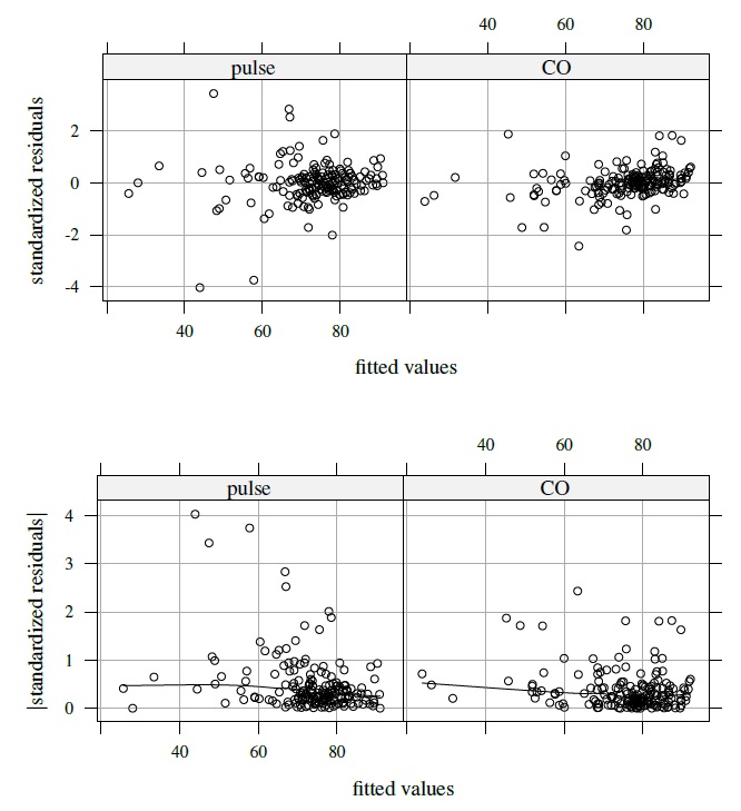
Figure 5.8 Plots of residuals (top panel) and their absolute values (bottom panel) against fitted values for each separate method in oximetry data. A nonparametric smooth is added to the bottom plots.
For evaluation of agreement, the estimates and 95% confidence bounds reported in Table 5.2 are, respectively, 0.85 and 0.80 for CCC and 10.9 and 12.1 for TDI (0.90).
Table 5.2 Summary of estimates of model parameters and measures of similarity, repeatability, and agreement for the oximetry data. Lower bounds for CCC and upper bounds for TDI are presented. Methods 1 and 2 refer to pulse oximetry and CO-oximetry, respectively.
| Parameter | Estimate | SE |
| β0 | 2.47 | 0.63 |
| μb | 73.17 | 1.47 |
| 4.74 | 0.20 | |
| log(ψ2) | 2.15 | 0.26 |
| log(σ2b*) | 2.45 | 0.19 |
| 2.75 | 0.17 | |
| 1.64 | 0.35 | |
| Similarity Evaluation | ||
| Measure | Estimate | 95% Interval |
| β0 | 2.47 | (1.23, 3.71) |
| λ | 3.04 | (1.32, 7.00) |
| Repeatability Evaluation | ||
| Measure | Estimate | 95% Bound |
| CCC1 | 0.82 | 0.76 |
| CCC2 | 0.88 | 0.83 |
| TDI1(0.90) | 12.13 | 13.48 |
| TDI2(0.90) | 9.51 | 10.60 |
| Agreement Evaluation | ||
| Measure | Estimate | 95% Bound |
| CCC | 0.85 | 0.80 |
| TDI(0.90) | 10.91 | 12.14 |
The TDI bound is about 17% of ![]() . It shows that 90% of the time the differences in measurements fall within ±12. These numbers suggest a weak agreement between the methods. Upon comparing the intra-and inter-method estimates for both measures, we come to the curious conclusion that the pulse method agrees more with the CO method than with itself! To explain this, one needs to look no further than the fitted distributions of D (CO-pulse difference) and D1 (pulse-pulse difference) given in (5.36) and (5.37), respectively. These distributions have comparable means but the variance of D1 is higher than D. Alternatively, one may verify that the condition given in Exercise 5.5 for inter-method agreement to exceed intra-method agreement holds with parameters replaced by estimates.
. It shows that 90% of the time the differences in measurements fall within ±12. These numbers suggest a weak agreement between the methods. Upon comparing the intra-and inter-method estimates for both measures, we come to the curious conclusion that the pulse method agrees more with the CO method than with itself! To explain this, one needs to look no further than the fitted distributions of D (CO-pulse difference) and D1 (pulse-pulse difference) given in (5.36) and (5.37), respectively. These distributions have comparable means but the variance of D1 is higher than D. Alternatively, one may verify that the condition given in Exercise 5.5 for inter-method agreement to exceed intra-method agreement holds with parameters replaced by estimates.
It is also apparent that the weak agreement between the methods is mostly due to their relatively poor repeatability. Transforming pulse measurements by adding ![]() to them makes the estimated fixed biases of the methods equal but does not help much with agreement. The CCC and TDI bounds improve slightly to 0.82 and 11.2, respectively. On the whole, we may prefer CO because of its higher precision than pulse, but CO’s precision itself is not as high as one would hope.
to them makes the estimated fixed biases of the methods equal but does not help much with agreement. The CCC and TDI bounds improve slightly to 0.82 and 11.2, respectively. On the whole, we may prefer CO because of its higher precision than pulse, but CO’s precision itself is not as high as one would hope.
We now assess the sensitivity of the results to the three observations of pulse identified earlier as outliers. For this we remove them and their paired counterparts to preserve the pairings, and repeat the analysis. This reduces pulse’s error standard deviation from 3.95 to 2.50, whereas the CO’s remains virtually unchanged (2.27 versus 2.25). It also reduces the estimate of λ, from 3.04 to 1.23, and its new confidence interval (0.53, 2.88) implies that the methods may be considered to have the same precision. The new confidence bounds for intra-method agreement of pulse and CO are, respectively, 0.82 and 0.83 for CCC and 11.05 and 10.71 for TDI. The same bounds for inter-method agreement are 0.81 for CCC and 11.41 for TDI. Note now that we do not have the situation of inter-method agreement being better than an intra-method agreement. Nonetheless, the closeness of intra-and inter-method agreement measures imply that the methods agree as well with themselves as with each other. This means we have no reason to prefer one method over the other on the basis of statistical considerations. However, the foregoing conclusions regarding modest agreement between the methods and their poor repeatability remain unchanged.
5.8 CHAPTER SUMMARY
- Repeated measurements may be unlinked, linked, or longitudinal. This distinction affects how the data are modeled. Only the first two types are covered in this chapter.
- The methodology developed here is appropriate for comparing methods with respect to their individual measurements rather than averages of the repeated measurements.
- The models assume equal scales for methods and homoscedasticity for errors.
- A subject × method interaction is incorporated in the models for both unlinked and linked data. The latter model additionally incorporates a subject × time interaction.
- Repeated measurements data allow reliable estimation of error variances of the methods. This is not possible with paired measurements data.
- With repeated measurements, one can also evaluate repeatability of a method, that is, intra-method agreement. If a method does not agree well with itself, it is unlikely to agree well with another method.
- A measure of inter-method agreement can be easily adapted to measure intra-method agreement.
- One normally expects the intra-method agreement of both methods to be higher than their inter-method agreement. But exceptions are possible, especially for linked data.
- Lack of agreement between two methods is often due to poor repeatability of one of the methods.
- Various measures of similarity, repeatability, and agreement are written as functions of model parameters, and the large-sample theory of ML estimators is used for inference on them.
- The methodology requires the number of subjects to be large for standard error estimates and confidence intervals to be accurate.
5.9 TECHNICAL DETAILS
In this section, we represent the mixed-effects models (5.1) and (5.9) for unlinked and linked repeated measurements data in the matrix notation introduced in Chapter 3.
5.9.1 Unlinked Data
Define
and

Let ![]() and
and
The matrix Ri depends on i through mi1 and mi2, the number of repeated measurements on subject i from the two methods. The matrix G is free of i. The model (5.1) can now be written as
where
It follows that
The elements of the mean vector Xiβ and the covariance matrix Vi are given earlier in (5.2)—(5.5) (Exercise 5.1). The vector of transformed parameters of this model is
5.9.2 Linked Data
Define Yi, ei, Xi, and Ri as before but with (mij, Mi) = (mi, 2mi). It is helpful to think of the times of measurement k = 1,...,mi, i = 1,...,n as the levels of a categorical time variable. Let ![]() be the number of its levels; only the first mi of which, namely, k = 1,...,mi, are observed for subject i. Alternatively, one can take
be the number of its levels; only the first mi of which, namely, k = 1,...,mi, are observed for subject i. Alternatively, one can take ![]() Redefine
Redefine ![]() as a (3 +
as a (3 + ![]() )-vector; G as a (3 +
)-vector; G as a (3 + ![]() ) × (3 +
) × (3 + ![]() ) diagonal matrix
) diagonal matrix
and Zi as an Mi × (3 + ![]() ) design matrix with the following characteristics:
) design matrix with the following characteristics:
its first three columns are

- the first and the last mi rows of its last
 columns are identical, and
 - each of them is an mi × whose leading mi × mi submatrix is an identity matrix, and the rest of the elements are zeros.
As in the unlinked case, G is free of i, but Ri depends on i through mi. We can now write the model (5.9) in the form (5.40) with
implying
The elements of the mean vector and covariance matrix here are given in (5.10)—(5.14) (Exercise 5.3). The vector of transformed parameters of this model is
The models (5.1) and (5.9) are fit by the ML method using a statistical software that fits mixed-effects models. Estimation of the various measures and standard errors of estimates and construction of confidence intervals and bounds proceed as described in Chapter 3.
5.10 BIBLIOGRAPHIC NOTE
A number of authors have discussed modeling and analysis of method comparison data with repeated measurements. Bland and Altman (1986, 1999, 2007) discuss computation of limits of agreement. They also present the intra-method counterpart of limits of agreement and term it the repeatability coefficient. However, they do not dwell on explicit modeling of data, which is the focus of Carstensen et al. (2008). Their models are similar but different from the ones in this chapter. This article is also the source of the oximetry data that we use for a case study. In addition, it introduces the terms linked and unlinked data that we adopt here. Such data were called paired and unpaired in an earlier paper by Chinchilli et al. (1996). Schluter (2009) presents a hierarchical Bayesian approach for analyzing repeated measurements data. Rather than modeling the individual measurements, Lai and Shiao (2005) directly model their differences using a mixed-effects model. Both Carstensen et al. (2008) and Lai and Shiao (2005) consider only the limits of agreement.
Several authors have considered variations of CCC for repeated measurements data. Chinchilli et al. (1996) propose a weighted CCC for both linked and unlinked scenarios. Their model is also a mixed-effects model, but they take a method of moments approach for estimation. Carrasco and Jover (2003) propose estimating CCC using the REML approach in a mixed-effects model framework, which is similar to ours. Barnhart et al. (2005) present intra-method, inter-method, and total-method versions of CCC for replicated data. Lin et al. (2007) also develop similar versions of various agreement measures, including CCC and TDI, under a mixed-effects model. Both articles use a GEE approach for estimation. Their definitions of inter-and intra-method agreement differs from ours. Quiroz (2005) develops equivalence tests based on CCC under a mixed-effects model for repeated measurements data. Chen and Barnhart (2008) compare CCC with various intraclass correlations under mixed-effects models. See also Carrasco et al. (2014).
The models in this chapter are special cases of those in Choudhary (2008). This article suggests bootstrap for inference if the number of subjects is not large, and also considers directly modeling differences of the paired measurements. Choudhary (2008), Quiroz and Burdick (2009), and Escaramis et al. (2010) discuss inference on TDI for repeated measurements data using mixed-effects models. Roy (2009) too considers such models but she focuses on inference on the measures of similarity.
Haber et al. (2005) introduce a new index based on inter-method and intra-method variability estimated from unlinked repeated measurements data. Haber and Barnhart (2008) introduce the notion of disagreement functions and use them to construct agreement measures that quantify inter-method agreement relative to intra-method agreement. They use a nonparametric approach for inference. Pan et al. (2012) propose a permutation-based agreement measure for unlinked data that compares observed disagreement between the methods to the agreement expected under individual equivalence—a condition under which the two methods have identical conditional distributions given a subject’s characteristics. They consider a nonparametric and a parametric method based on model (5.1) for inference on their measure.
The models (5.1) and (5.9) are for basic repeated measurements data. Often, however, the data are more complex and require variations and extensions of these models that incorporate additional structures present in the data. One example is the neognathae data from Igic et al. (2010), the same study that collected the kiwi data. But unlike the kiwi data where all eggs are from birds of a single species, these data come from eggs of 18 birds, two birds from each of the nine species considered. To take into account that the birds are nested within species, the model (5.1) is extended to incorporate a random species effect. Further variations and extensions of (5.1) are employed in Brulez et al. (2014) to evaluate repeatability of visual scoring methods of eggshell patterns, for example, spot size and pigment intensity, of two passerines, great tits and blue tits.
Data Source
The kiwi data are from Igic et al. (2010). They are presented in Table 5.3. Carstensen et al. (2008) is the source of the oximetry data. They are available in the R package MethComp of Carstensen et al. (2015).
Table 5.3 Kiwi data consisting of eggshell thickness measurements (in μm). They are provided by P. Cassey, see Igic et al. (2010).
| ID | Micrometer | Microscope |
| 1 | 300, 301, 296 | 318, 317, 322 |
| 2 | 315, 301, 304 | 318, 310, 312 |
| 3 | 356, 350, 350 | 385, 370, 380 |
| 4 | 435, 400, 421 | 431, 447, 447 |
| 5 | 296, 280, 270 | 298, 311, 316 |
| 6 | 320, 325, 310 | 331, 339, 305 |
| 7 | 320, 345, 310 | 335, 332, 331 |
| 8 | 358, 360, 359 | 332, 335, 324 |
| 9 | 250, 241, 241 | 272, 259, 276 |
| 10 | 315, 330, 329 | 336, 336, 352 |
| 11 | 268, 255, 270 | 283, 287, 275 |
| 12 | 301, 302, 300 | 306, 297, 291 |
| 13 | 220, 220, 200 | 229, 236, 244 |
| 14 | 325, 312, 310 | 318, 287, 289 |
| 15 | 355, 365, 353 | 360, 363, 371 |
| 16 | 311, 310, 302 | 327, 335, 337 |
EXERCISE
- Show that the marginal distribution of the vector Yi of unlinked observations on subject i (i = 1,...,n) is given by (5.41). Show also that the elements of the mean vector and covariance matrix of Yi are given by (5.2)—(5.5).
- Consider unlinked repeated measurements data associated with the model (5.1). The companion models for Yj and
 (j = 1, 2) are given by (5.6) and (5.23).
- Show that the marginal distribution of (Y1, Y2) is given by (5.7). Deduce the distribution of D given in (5.8).
- Show that the marginal distributions of (Yj, ) are given by (5.24) for j = 1 and (5.25) for j = 2. Deduce the distributions of Dj given in (5.26).
- Verify the expressions for intra-method CCC and TDI given in (5.27).
- What is the joint distribution of
 ?
?
- Repeat Exercise 5.1 for the linked case. In particular, show that the marginal distribution of the vector Yi of linked observations on subject i (i = 1,...,n) is given by (5.42). Show also that the elements of the mean vector and covariance matrix of Yi are given by (5.10)—(5.14).
- This is an analog of Exercise 5.2 for linked repeated measurements data that are modeled by (5.9). The companion models for Yj and
 (j = 1, 2) are given by (5.15) and (5.29).
- Show that the marginal distribution of (Y1, Y2) is given by (5.16). Deduce the distribution of D given in (5.17).
- Show that the marginal distributions of (Yj, ) are given by (5.30) for j = 1 and (5.31) for j = 2. Deduce the distributions of Dj given in (5.32).
- Verify the expressions for intra-method CCC and TDI given in (5.33).
- What is the joint distribution of ?
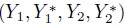
- Can a method, say, method 1, agree more with another method than with itself? The answer depends on the data model and the agreement measure considered. This exercise explores this issue assuming model (5.1) for unlinked data and (5.9) for linked data, and TDI and CCC as agreement measures. With these measures, higher inter-method agreement than intra-method agreement of method 1 means TDI(p) < TDI1(p) and CCC > CCC1. To simplify matters, assume that β0 = 0 so that the inter-method agreement is solely determined by the variance components. It may be noted that a nonzero β0 will lead to worse inter-method agreement than when β0 = 0. The intra-method agreement is not affected by β0.
- In the unlinked case, show that
Argue that the conditions on the right are unlikely to hold in practice.
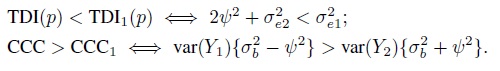
- In the linked case, show that
(The conditions on the right hold for parameter estimates based on the original oximetry data; see Section 5.7.2.) When
 , these conditions are equivalent to the condition that
  .
.
- In the unlinked case, show that
- Consider the kiwi data from Section 5.7.1.
- Fit model (5.1) to the data and verify the results in Table 5.1.
- Perform model diagnostics to verify the normality assumption for errors and random effects.
- Use the bootstrap approach described in Section 3.3.4 to compute analogs of the confidence intervals and bounds reported in Table 5.1. Compare the two sets of results.
- Consider the oximetry data from Section 5.7.2.
- The knee joint angle (in degrees) in a joint position called “full passive extension” is measured three consecutive times in 29 subjects using each of two goniometers. One is a Lamoreux-type electrogoniometer and the other is a plastic manual goniometer. The data are presented in Table 5.4. Assume unlinked repeated measurements.
- Perform an exploratory analysis of the data. Do you notice any outliers?
- Fit model (5.1) and check its adequacy. In particular, does the homoscedasticity assumption seem appropriate, possibly after removing outliers, if any?
- Evaluate similarity and repeatability of the methods.
- Evaluate agreement between the methods. Is the agreement high enough to justify using the methods interchangeably, possibly after a recalibration?
- Assess the impact of outliers, if any, on your conclusions.
- Cardiac ejection fraction (in %) is measured in 12 individuals using two methods—impedance cardiography (IC) and radionuclide ventriculography (RV). The data are presented in Table 5.5. Both methods have an equal number of repeated measurements on an individual, but this number varies between 3 and 6. Assume that the repeated measurements are paired over time, and they are taken in the order they appear in the table.
- Perform an exploratory analysis of the data.
- Fit model (5.9) and check its adequacy.
Table 5.4 Knee joint angle (in degrees) data for Exercise 5.8.
Subject Electro Manual 1 2, 1, 1 -2, 0, 1 2 12, 14, 13 16, 16, 15 3 4, 4, 4 5, 6, 6 4 9, 7, 8 11, 10, 10 5 5, 6, 6 7, 8, 6 6 -9, -10, -9 -7, -8, -8 7 17, 17, 17 18, 19, 19 8 5, 5, 5 4, 5, 5 9 -7, -6, -5 0, -3, -2 10 1, 2, 1 0, 0, -2 11 -4, -3, -3 -3, -2, -2 12 -1, -2, 1 3, -1, 1 13 4, 4, 2 7, 9, 9 14 -8, -10, -9 -6, -7, -6 15 -2, -2, -3 1, 1, 0 16 -12, -12, -12 -13, -14, -14 17 -1, 0, 0 2, 1, 0 18 7, 6, 4 4, 4, 3 19 -10, -11, -10 -10, -9, -10 20 2, 8, 8 8, 9, 8 21 8, 7, 7 7, 6, 7 22 -5, -5, -5 -3, -2, -4 23 -6, -8, -7 -5, -5, -7 24 3, 4, 4 5, 5, 5 25 -4, -3, -4 0, -1, -1 26 4, 4, 4 7, 6, 6 27 -10, -11, -10 -8, -8, -8 28 1, -1, 0 1, 1, 2 29 -5, -4, -5 -3, -3, -3 Adapted from Eliasziw et al. (1994), © 1994 American Physical Therapy Association, with permission from American Physical Therapy Association.
Table 5.5 Cardiac ejection fraction (in %) data for Exercise 5.9 (data provided by L. S. Bowling, see Bowling et al., 1993).
Subject IC RV 1 6.57, 5.62, 6.9, 6.57, 6.35 7.83, 7.42, 7.89, 7.12, 7.88 2 4.06, 4.29, 4.26, 4.09 6.16, 7.26, 6.71, 6.54 3 4.71, 5.5, 5.08, 5.02, 6.01, 5.67 4.75, 5.24, 4.86, 4.78, 6.05, 5.42 4 4.14, 4.2, 4.61, 4.68, 5.04 4.21, 3.61, 3.72, 3.87, 3.92 5 3.03, 2.86, 2.77, 2.46, 2.32, 2.43 3.13, 2.98, 2.85, 3.17, 3.09, 3.12 6 5.9, 5.81, 5.7, 5.76 5.92, 6.42, 5.92, 6.27 7 5.09, 4.63, 4.61, 5.09 7.13, 6.62, 6.58, 6.93 8 4.72, 4.61, 4.36, 4.2, 4.36, 4.2 4.54, 4.81, 5.11, 5.29, 5.39, 5.57 9 3.17, 3.12, 2.96 4.48, 4.92, 3.97 10 4.35, 4.62, 3.16, 3.53, 3.53 4.22, 4.65, 4.74, 4.44, 4.5 11 7.2, 6.09, 7, 7.1, 7.4, 6.8 6.78, 6.07, 6.52, 6.42, 6.41, 5.76 12 4.5, 4.2, 3.8, 3.8, 4.2, 4.5 5.06, 4.72, 4.9, 4.8, 4.9, 5.1 Reprinted from Bland and Altman (1999) with permission from SAGE.
- Evaluate similarity and repeatability of the methods using appropriate measures.
- Evaluate agreement between the methods. Do the methods agree sufficiently well to be used interchangeably? If not, is there any recalibration that may bring them closer?
- Table 5.6 provides measurements of peak expiratory flow rate (in l/min) made using a Wright peak flow meter and a mini Wright meter. Two measurements are taken by each meter on every subject. These data are from Bland and Altman (1986). They were collected to give a wide range of measurement, and are not representative of any population. Assume that the repeated measurements are unlinked. Analyze these data along the lines of the kiwi data case study discussed in Section 5.7 and Exercise 5.6.
Table 5.6 Peak expiratory flow rate (in l/min) data for Exercise 5.10.
Subject Wright Mini 1 494, 490 512, 525 2 395, 397 430, 415 3 516, 512 520, 508 4 434, 401 428, 444 5 476, 470 500, 500 6 557, 611 600, 625 7 413, 415 364, 460 8 442, 431 380, 390 9 650, 638 658, 642 10 433, 429 445, 432 11 417, 420 432, 420 12 656, 633 626, 605 13 267, 275 260, 227 14 478, 492 477, 467 15 178, 165 259, 268 16 423, 372 350, 370 17 427, 421 451, 443 Reprinted from Bland and Altman (1986), © 1986 The Lancet, with permission from Elsevier.
- Coronary artery calcium score is a measure of severity of arteriosclerosis, a risk factor for coronary heart disease. Two radiologists—A and B—make two replicate measurements of calcium score in 12 patients using the AJ-130 method. The data are given in Table 5.7. The repeated measurements are unlinked. Analyze these data.
Table 5.7 Coronary artery calcium score data for Exercise 5.11.
Subject A B 1 7, 6 6, 6 2 29, 31 30, 30 3 1, 1 0, 0 4 5, 6 5, 5 5 38, 32 40, 40 6 40, 29 30, 29 7 53, 49 50, 51 8 23, 23 23, 24 9 70, 70 70, 70 10 16, 15 16, 16 11 114, 116 120, 120 12 43, 43 43, 43 Reprinted from Haber et al. (2005) with permission from M. Haber.
- Consider the visceral fat data from the R package MethComp of Carstensen et al. (2015). They consist of measurements of thickness of visceral fat layer (in cm) in 43 patients taken by two observers—KL and SL. Each measurement is replicated three times. The repeated measurements are unlinked. Analyze these data.