CHAPTER 8
DATA WITH COVARIATES
8.1 PREVIEW
So far the method comparison data were assumed to solely consist of observations from the measurement methods of interest on a number of subjects. Frequently, however, additional data on a number of influential covariates are also available. These covariates may be categorical or continuous quantities and may affect either the means or the variances of the methods. This chapter coalesces ideas from previous chapters to present a unified method that incorporates covariates in the analysis. Both unreplicated and repeated measurements data are considered. As before, our approach is to first model the data and then use the assumed model for evaluating similarity and agreement, and possibly repeatability as well. A case study illustrates the methodology.
8.2 INTRODUCTION
Quite often in a method comparison study, data are collected on a number of covariates in addition to the observations from the measurement methods of interest. The covariates may be categorical or continuous. They are fixed, known quantities and are assumed to be measured without error. They include subject-level covariates, for example, gender of the subject, and method-level covariates. Of course, we always have the “measurement method” itself as a method-level categorical covariate in the analysis. The other covariates may affect the means of the methods, thereby explaining a portion of the variability in the measurements. We refer to them as the mean covariates. Incorporating them in the analysis adjusts the extent of agreement between the methods to account for their effects. A subset of the covariates may also interact with the methods in that the difference between the means of two methods depends on the covariates. In this case, the extent of agreement depends on the covariates. It may also be that the variance of a measurement method, particularly its error variance, depends on covariates. Such covariates are called variance covariates (as we saw in Chapter 6). Even in this case, the extent of agreement depends on the covariates. Thus, there is a clear need for identifying covariates and incorporating them in the analysis.
Let the study have r mean covariates, x1,..., xr, not including the effects of measurement methods. Each contributes one or more explanatory variables to the mean model. A categorical covariate with L levels is represented using L − 1 indicator explanatory variables. A continuous covariate may be included either on the original scale or on a transformed scale. Let x be the vector of all explanatory variables contributed by the r covariates, including the main effects as well as the interactions of interest. Let ![]() be a variance covariate that may depend on the mean covariates. It is taken to be a scalar quantity that can be continuous or categorical. The ranges of the covariates are taken to be their observed ranges in the data.
be a variance covariate that may depend on the mean covariates. It is taken to be a scalar quantity that can be continuous or categorical. The ranges of the covariates are taken to be their observed ranges in the data.
We assume that the study involves J (≥ 2) methods with single measurements or repeated measurements that may be linked or unlinked. The covariates do not change with time. Time-dependent covariates are discussed in Chapter 9 on longitudinal data. As before, let Yij, j = 1,..., J, i = 1 ,..., n denote the unreplicated data, and Yijk, k = 1,...,mij , j = 1,..., J, i = 1 ,..., n denote the repeated measurements data. Here i is the subject index, j is the method index, and k indexes the order in which the repeated measurements are taken. We use Mi to denote the number of observations on subject i. It equals J for unreplicated data and ![]() mij for repeated measurements data. Let
mij for repeated measurements data. Let ![]() Mi. Also, let (x1i,..., xri), xi, and
Mi. Also, let (x1i,..., xri), xi, and ![]() , respectively, denote for subject i the values of the vector of mean covariates (x1,...,xr), the vector of explanatory variables x, and the variance covariate
, respectively, denote for subject i the values of the vector of mean covariates (x1,...,xr), the vector of explanatory variables x, and the variance covariate ![]() .
.
As in previous chapters, we take a model-based approach. We include mean and variance covariates in the model and base our inferences on the expanded model.
8.3 MODELING OF DATA
We first discuss how the population means and variances of the methods can be modeled as functions of covariates.
8.3.1 Modeling Means of Methods
The population means of the methods have been assumed to be constants thus far. In particular, the mean µj of method j has the form
where β0j can be written in terms of model parameters (Exercise 8.1). We now let these means be functions of the explanatory variables x as in a linear regression analysis. The mean functions are linear in regression coefficients and are parametric in that they have specified functional forms. The forms are assumed to be the same for all the J methods to allow the data from different methods to have marginal distributions of the same form. As before, method 1 serves as the reference method. Two scenarios arise depending on whether or not covariates interact with the methods.
8.3.1.1 No Method X Covariates Interaction
When none of the covariates interacts with the methods, we can write the mean function for the jth method as
where β0j are intercepts and β1 is a vector of slope coefficients associated with x. Only the intercepts here depend on j; the slopes are free of j because there is no interaction with the method. It follows that the difference in mean functions of methods j and l with identical covariate data is
which does not depend on the covariates.
8.3.1.2 Method X Covariates Interaction
Suppose some of the r covariates interact with the methods. Let xI be the s × 1 vector of the interacting variables. The mean function for method j can be expressed as
where βIj is the s × 1 vector of regression coefficients associated with xI and depends on j due to the interaction. Moreover, because method 1 serves as the reference, its coefficients for the interacting variables are assumed to be zero, that is,
This assumption is necessary to enforce identifiability. The difference in mean functions of methods j and l is
The model (8.3) is a generalization of the model (8.1) and it reduces to the latter when there is no interaction, that is, βIj = 0 for all j . In this case, the differences (8.2) and (8.4) are identical. The general form (8.3) is used in the subsequent sections.
8.3.2 Modeling Variances of Methods
Ideally, to model variances of the methods in terms of the variance covariate ![]() , we model the error variances of the methods. However, we have seen earlier that reliable estimation of error variances requires either repeated measurements data or unreplicated data on more than two methods. In particular, the estimates are not reliable for paired measurements data in which case we can only model the overall variances. This suggests that we must consider the two scenarios separately.
, we model the error variances of the methods. However, we have seen earlier that reliable estimation of error variances requires either repeated measurements data or unreplicated data on more than two methods. In particular, the estimates are not reliable for paired measurements data in which case we can only model the overall variances. This suggests that we must consider the two scenarios separately.
Assume for now that we have repeated measurements data on J (≥ 2) methods. If ![]() is continuous, we can proceed exactly as in Chapter 6 to model error variances as functions of
is continuous, we can proceed exactly as in Chapter 6 to model error variances as functions of ![]() , that is,
, that is,
where gj is a specified variance function for method j that depends on the heteroscedasticity parameter vector δj and has the property that gj(![]() , 0) = 1. When δ1 = ... = δJ = 0, the model becomes homoscedastic. In practice, the variance functions gj in (8.5) may be taken to be the same for all methods. In this case, it may also be reasonable to impose some structure on the heteroscedasticity parameters. For example, they may be assumed to identical, that is, δ1 = ... = δJ, but having a nonzero value. The model (8.5) is same as (6.9) except that J can be more than two here, and the covariate is not necessarily a proxy for the magnitude of measurement. Thus, the discussion in Section 6.4 about how to specify the variance functions and evaluate their adequacy is relevant here as well.
, 0) = 1. When δ1 = ... = δJ = 0, the model becomes homoscedastic. In practice, the variance functions gj in (8.5) may be taken to be the same for all methods. In this case, it may also be reasonable to impose some structure on the heteroscedasticity parameters. For example, they may be assumed to identical, that is, δ1 = ... = δJ, but having a nonzero value. The model (8.5) is same as (6.9) except that J can be more than two here, and the covariate is not necessarily a proxy for the magnitude of measurement. Thus, the discussion in Section 6.4 about how to specify the variance functions and evaluate their adequacy is relevant here as well.
Suppose now that ![]() is a categorical variable with L levels and the error variance of method j changes with the level of
is a categorical variable with L levels and the error variance of method j changes with the level of ![]() . The JL error variances can be written as
. The JL error variances can be written as
However, this model has J + JL parameters, implying the need to impose J constraints on the parameters to make the model identifiable. One can assume
which amounts to interpreting the heteroscedasticity parameters ![]() for l =2,..., L as the ratio of error variances of method j under the lth and the first settings of the covariate
for l =2,..., L as the ratio of error variances of method j under the lth and the first settings of the covariate ![]() . The model is homoscedastic when all
. The model is homoscedastic when all ![]() are one. Also, as in the continuous case, some structure may be imposed on these heteroscedasticity parameters. The model (8.6) can be seen to be a special case of the model (8.5) by taking
are one. Also, as in the continuous case, some structure may be imposed on these heteroscedasticity parameters. The model (8.6) can be seen to be a special case of the model (8.5) by taking
as the variance function and
as the vector of heteroscedasticity parameters. The general model (8.5) is used in the subsequent sections.
The above discussion has assumed repeated measurements data. Nonetheless, the model (8.5) can also be used for modeling error variances in the case of unreplicated data from J ( > 2) methods, provided, of course, that var(eijk) is replaced with var(eij). As seen in Section 6.5, upon replacing var(eijk) with var(Yij), it can also be used for modeling overall variances of measurements when we have paired measurements data.
8.3.3 Data Models
Our task now is to generalize the data models of previous chapters by integrating them with the mean function model (8.3) in terms of the covariates x1,...,xr, and the variance function model (8.5) in terms of the covariate ![]() . The specific models to be generalized are as follows: the bivariate normal model (4.6) for paired data; the mixed-effects model (7.1) for unreplicated data from J > 2 methods; the mixed-effects models (5.1) and (5.9) for unlinked and linked repeated measurements data from J = 2 methods; and the extensions (7.4) and (7.14) of (5.1) and (5.9) for J > 2 methods. The new models are formulated in general terms. In practice, one has to go through the usual model building exercise to find which covariates, if any, are significant for modeling either the means or the variances, and hence should be included in the model. Setting βIj = 0 for all j in the new models gives their versions without the method × covariate interaction. Homoscedastic versions are obtained by setting δj = 0 for all j. Setting β1 and βIj and δj for all j equal to 0 gives back the versions without the covariates.
. The specific models to be generalized are as follows: the bivariate normal model (4.6) for paired data; the mixed-effects model (7.1) for unreplicated data from J > 2 methods; the mixed-effects models (5.1) and (5.9) for unlinked and linked repeated measurements data from J = 2 methods; and the extensions (7.4) and (7.14) of (5.1) and (5.9) for J > 2 methods. The new models are formulated in general terms. In practice, one has to go through the usual model building exercise to find which covariates, if any, are significant for modeling either the means or the variances, and hence should be included in the model. Setting βIj = 0 for all j in the new models gives their versions without the method × covariate interaction. Homoscedastic versions are obtained by setting δj = 0 for all j. Setting β1 and βIj and δj for all j equal to 0 gives back the versions without the covariates.
In what follows, the mean function µj (x1i,...,xri) is given by (8.3) with x and xI replaced by their respective values xi and xIi for subject i. Moreover, the mean difference function ξjl(x1,...,xr) is given by (8.4).
8.3.3.1 Repeated Measurements Data
Consider the model (7.4) for unlinked data from J > 2 methods. It assumes β1 = 0 for identifiability. We make three changes to the model. First, we write the term βj + bi in an equivalent form, β0j + ui, where ui = bi − µb and β0j = βj + µb. The ui represents the centered true value for subject i and β0j represents the mean µj of method j. Next, we replace the constant mean with the mean function (8.3). Finally, the constant error variance ![]() is replaced by the variance function (8.5). Thus, the model (7.4) generalizes to
is replaced by the variance function (8.5). Thus, the model (7.4) generalizes to
where
The other terms in (8.7) and the assumptions regarding them remain the same as in (7.4). The assumptions imply that the vector of Mi observations on subject i follows an independent Mi-variate normal distribution with
and the covariances, free of the covariates, are given by (7.6) and (7.7); see Exercise 8.2. It also follows from this exercise that the joint distribution of the population vector (Y1, ...,YJ) induced by the model (8.9) at covariate setting (x1, ...,xr, ![]() ) is a J-variate normal distribution with
) is a J-variate normal distribution with
for j ≠ l. Therefore, for the difference Djl = Yl − Yj we have
with
These distributions are used to derive measures of similarity and agreement. Moreover, as in Section 7.6.1, the distribution of the measurement pair (Yj, ![]() ) from method j is bivariate normal with identical marginals (Exercise 8.2). Therefore, for j = 1, ...,J, the mean and variance of
) from method j is bivariate normal with identical marginals (Exercise 8.2). Therefore, for j = 1, ...,J, the mean and variance of ![]() are same as those of Yj given in (8.10). Further, we can see that
are same as those of Yj given in (8.10). Further, we can see that
and
These distributions are needed to derive measures of repeatability.
For linked data from J (> 2) methods, we generalize the model (7.14) to write
where the distributions of ui and eijk are given by (8.8), and the rest of the terms are from (7.14). Exercise 8.3 derives the marginal distribution of these data. It also shows that the joint distribution of (Y1, ...,YJ) at (x1, ...,xr, ![]() ) is a J-variate normal distribution with E(Yj) = µj (x1, ...,x r),
) is a J-variate normal distribution with E(Yj) = µj (x1, ...,x r),
The distribution of the difference Djl is the same as in unlinked data and is given by (8.11). Further, it can be seen that (Yj, ![]() ) follows a bivariate normal distribution with identical marginals and covariance given by (8.13). For the distribution of their difference Dj, we have
) follows a bivariate normal distribution with identical marginals and covariance given by (8.13). For the distribution of their difference Dj, we have
Thus far in this section we assumed J > 2. Under this assumption, the variance ψj2 of subject × method interaction is allowed to depend on method (Section 7.6). All results hold for J = 2 as well, provided ψj2 for all j is replaced by a common variance ψ2 (Exercise 8.4). In particular, the model for unlinked repeated measurements data from J = 2 methods is
and its counterpart for linked data is
where
All other assumptions are same as in the J > 2 case. These models generalize the models (5.1) and (5.9) for unlinked and linked data, respectively. The model (8.18) also generalizes the heteroscedastic model (6.10) by not restricting the variance covariate to be a proxy for the true measurement and additionally allowing mean covariates in the model. The distributions of the various model-based quantities, for example, (Y1, Y2), D12, ![]() ,
, ![]() , D1, and D2, under (8.18) and (8.19) can be obtained from their counterparts for J > 2 by simply setting
, D1, and D2, under (8.18) and (8.19) can be obtained from their counterparts for J > 2 by simply setting ![]() .
.
8.3.3.2 Unreplicated Data from More Than Two Methods
The model (7.1) is extended as
The distributions of ui and eij are given by (8.8) with eij replacing eijk. Marginal distribution of the data under this model is obtained in Exercise 8.5. It is also seen that the joint distribution of (Y1, ...,YJ) at (x1, ...,xr, ![]() ) is a J-variate normal with E(Yj) = µj(x1, ...,xr) and covariance structure described by
) is a J-variate normal with E(Yj) = µj(x1, ...,xr) and covariance structure described by
The distribution of the difference Djl is
where
8.3.3.3 Paired Measurements Data
Proceeding as before, but using the variance function in (8.5) to model var(Yj), the bivariate normal distribution (4.6) of (Y1, Y2) at covariate value (x1, ..., xr, ![]() ) is replaced by the assumption
) is replaced by the assumption
 (8.24)
Thus, the observed pairs (Yi1, Yi2) are independently distributed as
 (8.25)
This model generalizes the heteroscedastic bivariate normal model (6.33) by letting the means depend on covariates. Here again the correlation ρ of the distribution is constant but the covariance depends on ![]() and heteroscedasticity parameters (δ1, δ2). Further,
and heteroscedasticity parameters (δ1, δ2). Further,
where
8.3.4 Model Fitting and Evaluation
The models introduced here need to be fit by the ML method using a statistical software package. For a given model, estimates of mean and variance functions are obtained by replacing the unknown parameters in them by their ML estimates. For the bivariate normal model, the estimated mean functions at the observed covariate values in the data also serve as the fitted values. For a mixed-effects model, the fitted values are obtained by adding the predicted values of the random effects to the estimated means. We obtain the residuals by subtracting the fitted values from the observed values and standardize them by dividing by their estimated standard deviations. These quantities are used for model evaluation (Section 3.2.4). It is important to check the adequacy of the assumed mean and variance function models. For the former, model diagnostics for a typical regression analysis can be carried out. For the latter, one can proceed as in Section 6.4.3 for a mixed-effects model and as in Section 6.5.3 for the bivariate normal model. The need for including a mean or a variance covariate in the model can be assessed using a likelihood ratio test or model comparison criterion (Section 3.3.7).
8.4 EVALUATION OF SIMILARITY, AGREEMENT, AND REPEATABILITY
For the evaluation of similarity and agreement, we proceed by combining ideas from Chapters 6 and 7. The distributions of (Y1,...,YJ) for J ≥ 2 obtained in Section 8.3.3 at a covariate setting (x1,..., xr,![]() ) can be used in the usual manner to derive measures of similarity and agreement. They are adjusted for mean covariates in the model. They are also functions of covariates if either a covariate × method interaction or a variance covariate is included in the model. Among the similarity measures, the analog of the difference in fixed biases or means of methods j and l is ξjl(x1,..., xr), given by (8.4). It reduces to β0l − β0j, simply a difference in intercepts if none of the covariates interact with the methods. Further, as in Section 6.4.5, the precision ratio for a mixed-effects model is
) can be used in the usual manner to derive measures of similarity and agreement. They are adjusted for mean covariates in the model. They are also functions of covariates if either a covariate × method interaction or a variance covariate is included in the model. Among the similarity measures, the analog of the difference in fixed biases or means of methods j and l is ξjl(x1,..., xr), given by (8.4). It reduces to β0l − β0j, simply a difference in intercepts if none of the covariates interact with the methods. Further, as in Section 6.4.5, the precision ratio for a mixed-effects model is
 (8.28)
Such a ratio is not defined for the bivariate normal model. Instead, as in Section 6.5.5, we use the variance ratio,
 (8.29)
The measures of agreement between methods j and l under a model are obtained by replacing the features of distributions of (Yj, Yl) and Djl used in their definitions by associated functions of model parameters (Exercise 8.6). However, the model depends on the study design, and hence we consider the various designs separately.
8.4.1 Measures of Agreement for Two methods
For unlinked repeated measurements data, the distributions of (Y1, Y2) and D12 are given by (8.10) and (8.11) with ![]() . By substituting their moments in (2.6) and (2.29) we obtain CCC12(x1, ..., xr,
. By substituting their moments in (2.6) and (2.29) we obtain CCC12(x1, ..., xr, ![]() ) as
) as
 (8.30)
and TDI12( p0, x1, ..., xr, ![]() ) as
) as
 (8.31)
where
For linked repeated measurements data, the distribution of (Y1, Y2) is given by (8.16) with ![]() . Using its moments in (2.6) we obtain CCC12(x1, ..., xr,
. Using its moments in (2.6) we obtain CCC12(x1, ..., xr, ![]() ) as
) as
 (8.33)
The distribution of D12 and hence the TDI function are identical to the unlinked case, given in (8.31).
For paired measurements data, the distributions of (Y1, Y2) and D12 are given by (8.24) and (8.26). Using their moments in the definitions of the agreement measures leads to
 (8.34)
and TDI12(p0, x1, ..., xr, ![]() ) as in (8.31), where
) as in (8.31), where ![]() is taken from (8.27).
is taken from (8.27).
8.4.2 Measures of Agreement for More Than Two Methods
For repeated measurements data, it follows directly from (2.6), (8.10), and (8.16) that CCCjl(x1, ..., xr, ![]() ) for unlinked and linked data are, respectively, given by
) for unlinked and linked data are, respectively, given by
 (8.35)
and
 (8.36)
It similarly follows from (2.29) and (8.11) that
 (8.37)
for both unlinked and linked data with ![]() given by (8.12).
given by (8.12).
For unreplicated data, we have
 (8.38)
from (2.6) and (8.21). We also see from (2.29) and (8.22) that TDIjl(p0, x1, ..., xr,, ![]() ) is given by (8.37), where
) is given by (8.37), where ![]() is taken from (8.23).
is taken from (8.23).
8.4.3 Measures of Repeatability
Measures of repeatability for evaluation of intra-method agreement for repeated measurements data are obtained using the distributions of (Yj, ![]() ) and Dj for j = 1, ..., J given in Section 8.3.3.1. Proceeding as in Sections 6.4.5 and 7.9, we get the repeatability analogs for CCC and TDI for unlinked data from J > 2 methods. They are
) and Dj for j = 1, ..., J given in Section 8.3.3.1. Proceeding as in Sections 6.4.5 and 7.9, we get the repeatability analogs for CCC and TDI for unlinked data from J > 2 methods. They are
 (8.39)
Their counterparts for linked data are
 (8.40)
These expressions are verified in Exercise 8.7. Expressions for the J = 2 case are obtained by replacing ψj2 in (8.39) and (8.40) with the common value ψ2. The resulting expressions are identical to (6.26) for unlinked data. Repeatability measures involve the variance covariate but not the mean covariates because their effects cancel out when Yj is compared with ![]() at the same covariate setting.
at the same covariate setting.
8.4.4 Inference on Measures
The measures are estimated by the ML method, and inference on them proceeds as described in Chapter 3. As usual, we use two-sided confidence intervals for measures of similarity and appropriate one-sided confidence bounds for measures of agreement and repeatability. Depending upon the objectives of the study, the bounds and intervals may be pointwise or simultaneous over specified method pairs or covariate values (see Section 3.3.5). If a measure is a function of a categorical covariate, it may be of interest to examine whether it can be taken to remain constant over the levels of the covariate. One can perform this task either using two-sided simultaneous confidence intervals for appropriately defined differences of the values of the measure or using a test of homogeneity that tests the null hypothesis of equality of the measure’s values (Section 3.3.6).
The 95 % limits of agreement for comparing methods j and l in all cases have the form
where ![]() and
and ![]() are the ML estimators of the mean and variance of the difference Djl. The repeatability analogs of this measure can be defined similarly.
are the ML estimators of the mean and variance of the difference Djl. The repeatability analogs of this measure can be defined similarly.
8.5 CASE STUDY
The methodology developed in this chapter is illustrated using a blood pressure dataset. The dataset consists of systolic blood pressure measurements of n = 384 subjects measured using a mercury sphygmomanometer (method 1) and an automatic monitor, OMRON 711 (method 2). Each subject is measured twice using each method. Thus, there is a total of 384 × 2 × 2 = 1536 blood pressure measurements. The replications are assumed to be unlinked. Three subject-level covariates—gender, age, and heart rate—are also recorded in the data. Gender is a categorical covariate with levels male and female. Age (in years) and heart rate (in beats per minutes) are continuous covariates. None of these covariates changes during replication. There are 196 female and 184 male subjects in the dataset and they are between 24 and 74 years of age. Their blood pressure ranges between 89 and 200 mm Hg. Their heart rate ranges between 43 and 160 beats per minute, with one subject at 160 and the rest at 121 or less.
Figure 8.1 presents separate trellis plots of data for each gender. The effect of gender is apparent at the low end of the measurement range where the males tend to have higher blood pressure than the females. Specifically, 99 is the smallest observation for the males, whereas 89 is the smallest for the females. There are 50 readings for females between 89 and 99. There are a handful of subjects with outlying observations. For example, among the four observations for the female in the topmost row, three are near 100 but one is near 200. We also see that the observations for the females from the mercury method tend to be a bit smaller than the automatic method. However, no such difference is apparent among the males. This provides evidence for a method × gender interaction. Next, the methods have comparable within-subject variations, but the variations appear to increase somewhat with the blood pressure level. Although these error variations appear small in relation to the between-subject variation, their magnitude is considerable. Figure 8.2 presents side-by-side boxplots of all measurements from the two methods for both genders. They corroborate the impressions regarding effect of gender and its interaction with method.
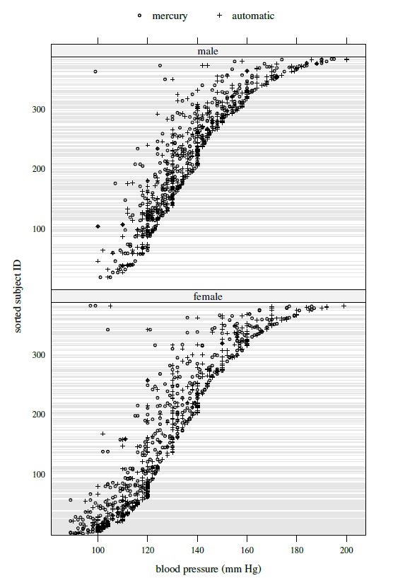
Figure 8.1 Trellis plots of blood pressure data by gender.
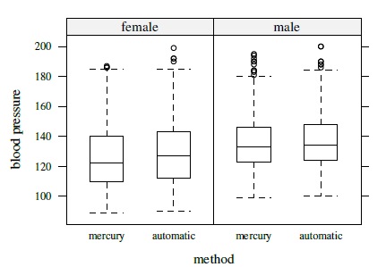
Figure 8.2 Side-by-side boxplots for blood pressure data by gender.
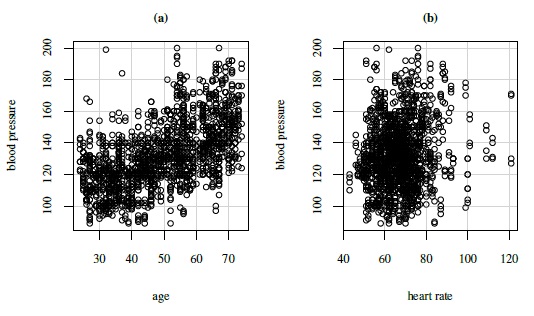
Figure 8.3 Scatterplots of blood pressure against age (left panel) and against heart rate (right panel).
Scatterplots of blood pressure against age and heart rate are presented in Figure 8.3. Blood pressure tends to increase with age. It also appears to have a mild positive correlation with heart rate. The latter plot excludes the subject with the unusually high heart rate of 160. The blood pressure readings for that subject, ranging from 146 to 155 mm Hg, are in the middle of the other values.
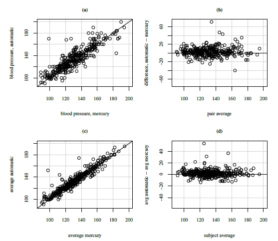
Figure 8.4 Plots for blood pressure data. Top panel (left to right): Scatterplot with line of equality and Bland-Altman plot with zero line based on randomly formed measurement pairs. Bottom panel (left to right): Same as top panel but based on average measurements.
Figure 8.4 displays scatterplots and Bland-Altman plots for the measurement pairs formed by randomly selecting one of the two replications of each method and also for the averages of the replications. The scatterplots show a moderately high correlation (0.87) between the measurements. The correlation is higher between the averages (0.95), but this is to be expected. Absence of any trend in the Bland-Altman plots suggest equal scales for the methods. All plots show a few outliers.
Our strategy is to first analyze the data without the covariates and then again with the covariates so that their impact on the results can be assessed. Therefore, first we fit the model (8.18) without any mean or variance covariates. This model is effectively the model (5.1). Evaluation of the fitted model reveals that the variance ψ2 of the subject × method interaction bij is practically zero. Besides, there are four standardized residuals with absolute values between 5 and 10 and the corresponding observations exert some influence on the error variance estimates. Therefore, these observations are deleted from all analysis hereafter. Upon refitting the model, we find clear evidence of magnitude-dependent heteroscedasticity in the methods (see Chapter 6). To incorporate this heteroscedasticity, we follow Section 6.4 to take the variance covariate ![]() i as the subject blood pressure average (6.20) and plot the log of the absolute residuals of the fitted model against log(
i as the subject blood pressure average (6.20) and plot the log of the absolute residuals of the fitted model against log(![]() i) separately for each method. The plots superimposed with fitted regression lines are displayed in Figure 8.5. The underlying trends in both plots can be approximated by a straight line, implying that the power model
i) separately for each method. The plots superimposed with fitted regression lines are displayed in Figure 8.5. The underlying trends in both plots can be approximated by a straight line, implying that the power model
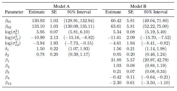
may be taken as the variance function models for both methods. Now these gj functions are used to fit the model (8.18) without any mean covariates, which is effectively the heteroscedastic model (6.10). The p-value of less than 0.001 for the likelihood ratio test of the null hypothesis δ1 = δ2 = 0 (Section 6.4.4) confirms the need for incorporating heteroscedasticity. The residual plots for the fitted model, shown in Figure 8.6, points to the adequacy of the power model for describing heteroscedasticity. Finally, we refit the model by deleting the interaction term bij from the model. The p-value of 0.99 for the likelihood ratio test of the null hypothesis ψ2 = 0 clearly justifies this deletion (Section 3.3.7). The ML estimates of parameters in the resulting model, called Model A, are presented in Table 8.1. They are virtually identical to the estimates for the previous model that includes the interaction (not shown).
Substituting the ML estimates in (8.3), (8.10), (8.11), and (8.12), we see that, under Model A, the fitted distributions of (Y1, Y2) and D12 at the blood pressure level ![]() are
are
 (8.42)
respectively. Here ![]() ranges over (89, 200) mm Hg, the observed measurement range in the data. The mercury method has a slightly smaller mean than the automatic method. The former’s error standard deviation, given by {(1.68 × 10⁻⁵)
ranges over (89, 200) mm Hg, the observed measurement range in the data. The mercury method has a slightly smaller mean than the automatic method. The former’s error standard deviation, given by {(1.68 × 10⁻⁵)![]() 3.00}1/2, increases from 3.4 to 11.5 and the same for the latter, given by {(1.95 × 10⁻²)
3.00}1/2, increases from 3.4 to 11.5 and the same for the latter, given by {(1.95 × 10⁻²)![]() 1.56}1/2, increases from 4.6 to 8.6. The two functions cross near
1.56}1/2, increases from 4.6 to 8.6. The two functions cross near ![]() = 135. These error standard deviations appear large relative to the magnitude of measurement. Nevertheless, they are dominated by the between-subject standard deviation of
= 135. These error standard deviations appear large relative to the magnitude of measurement. Nevertheless, they are dominated by the between-subject standard deviation of ![]() As a result, the overall standard deviations of both the methods show relatively little change over the measurement range—they vary between 20 and 23. Correlation between the methods, obtained using (8.42), decreases from 0.96 to 0.79. The mean of the difference in the measurements is 2.18 and its standard deviation increases from 5.7 to 14.4. Taken together, these results indicate somewhat weak intra-and inter-method agreement.
As a result, the overall standard deviations of both the methods show relatively little change over the measurement range—they vary between 20 and 23. Correlation between the methods, obtained using (8.42), decreases from 0.96 to 0.79. The mean of the difference in the measurements is 2.18 and its standard deviation increases from 5.7 to 14.4. Taken together, these results indicate somewhat weak intra-and inter-method agreement.
Our next task is to assess the effects of the three covariates—gender, age, and heart rate (labeled rate)—for inclusion in Model A as mean covariates. A standard model building exercise shows that the main effects of all three as well as gender × age and gender × method interactions are statistically significant, with p-values well under 0.05, and should be included. In the expanded model, called Model B, the mean functions (8.3) of the mercury (method 1) and automatic (method 2) methods are modeled as follows:
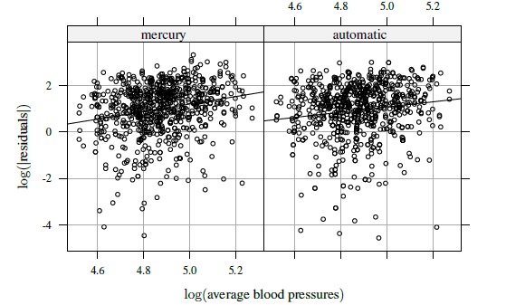
Figure 8.5 Plots of log of absolute residuals from a homoscedastic fit to blood pressure data against log( ) with as subject average blood pressure. A simple linear regression fit is superimposed on each plot.
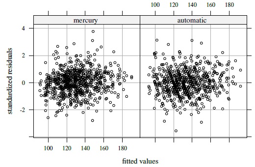
Figure 8.6 Residual plots from a heteroscedastic fit to blood pressure data using power variance function models.
Table 8.1 Summary of estimates of parameters of Models A (with variance covariate) and B (with mean and variance covariates) for blood pressure data. Methods 1 and 2 refer to mercury sphygmomanometer and automatic monitor, respectively.
 (8.43)
The rest of this model is identical to Model A. Table 8.1 provides estimates of the regression coefficients in (8.43) as well as other model parameters. The estimates of β01 and β02 show substantial change from Model A after accounting for variability in the blood pressure measurements due to the mean covariates. This also reduces the heterogeneity between the subjects vis-à-vis their blood pressure measurements, leading to a decrease in the estimate of ![]() . The estimates of
. The estimates of ![]() and
and ![]() decrease somewhat, while the estimates b of δ1 and δ2 increase slightly. In addition, there is a significant gender × method interaction effect βI2.
decrease somewhat, while the estimates b of δ1 and δ2 increase slightly. In addition, there is a significant gender × method interaction effect βI2.
A substitution of the estimates in (8.43) gives the fitted mean functions as
 (8.44)
The signs of the regression coefficients show that the mean blood pressure increases with age and also that blood pressure and heart rate are positively correlated. These findings are consistent with what we saw in Figure 8.3. To see the effect of gender, we can write the mean differences from (8.44) as
These differences obviously depend on age because of the gender × age interaction. Over the observed age interval of 24 to 74 years, the first difference decreases from 21.8 to 0.8, and the second difference decreases from 19.5 to 0 until age 70; thereafter it falls slightly below 0 to −1.5. While this finding confirms the observation that males tend to have higher blood pressure than females (Figure 8.2), it additionally shows that their mean difference decreases with age and essentially vanishes around age 70. This is true regardless of the method used for measuring blood pressure.
As in (8.42), the fitted distributions of (Y1, Y2) and D12 under Model B are also normal distributions. But their means now depend on the covariates values. Mean functions of the bivariate distribution are given in (8.44). The covariance matrix of the distribution is
 (8.45)
The mean function of the difference in the methods is
 (8.46)
Further, from (8.12), its variance function can be seen to be
The mean in (8.46) depends on gender because of the gender × method interaction, but is free of age and rate effects (see Section 8.3.1). Its value is 3.19 for females and 0.90 for males. The magnitudes and directions of these values are consistent with what we saw in Figures 8.1 and 8.2. The error standard deviation of the mercury method, given by {(9.09 × 10⁻⁶)![]() 3.11}1/2, increases from 3.3 to 11.7, and the same for the automatic method, given by {(9.92 × 10⁻³)
3.11}1/2, increases from 3.3 to 11.7, and the same for the automatic method, given by {(9.92 × 10⁻³)![]() 1.69}1/2, increases from 4.5 to 8.9. The overall standard deviations of these methods range from 14.8 to 18.6 and 15.1 to 17.0, respectively, and their correlation decreases from 0.93 to 0.66. Furthermore, the standard deviation of the difference in the methods ranges from 5.6 to 14.7. The 95 % limits of agreement as functions of
1.69}1/2, increases from 4.5 to 8.9. The overall standard deviations of these methods range from 14.8 to 18.6 and 15.1 to 17.0, respectively, and their correlation decreases from 0.93 to 0.66. Furthermore, the standard deviation of the difference in the methods ranges from 5.6 to 14.7. The 95 % limits of agreement as functions of ![]() can be computed using (8.41).
can be computed using (8.41).
Upon comparing these Model B results with those under Model A, we see that the earlier mean difference ![]() 12 of 2.18 between the methods now falls between the values 0.90 for males and 3.19 for females. That said, the difference between the three values may not be considered practically important. The error variations of the methods, although given by seemingly different functions, remain very similar under the two models. However, the between-subject variation decreases from 384.9 to 209.4, causing notable reductions in the overall variances of the methods and also in their correlation.
12 of 2.18 between the methods now falls between the values 0.90 for males and 3.19 for females. That said, the difference between the three values may not be considered practically important. The error variations of the methods, although given by seemingly different functions, remain very similar under the two models. However, the between-subject variation decreases from 384.9 to 209.4, causing notable reductions in the overall variances of the methods and also in their correlation.
We next proceed to the evaluation of similarity, agreement, and repeatability of the methods. For the measures that do not depend on the variance covariate ![]() , we report 95% individual confidence bounds or intervals. For those that do, 95% simultaneous one-or two-sided confidence bands computed on a grid of 30 equally spaced points in (89, 200) are reported. To evaluate similarity, we just recall that the estimates of the mean difference ξ12 are: 2.18 for Model A, and 0.90 for males and 3.19 for females in the case of Model B. The corresponding 95% confidence intervals are (1.57, 2.78), (0, 1.80), and (2.39, 3.99), respectively. Although these differences are either clearly statistically significant or on the borderline, none of the confidence limits is large from a practical viewpoint. Figure 8.7 presents estimates and 95% confidence bands for the precision ratio function λ12(
, we report 95% individual confidence bounds or intervals. For those that do, 95% simultaneous one-or two-sided confidence bands computed on a grid of 30 equally spaced points in (89, 200) are reported. To evaluate similarity, we just recall that the estimates of the mean difference ξ12 are: 2.18 for Model A, and 0.90 for males and 3.19 for females in the case of Model B. The corresponding 95% confidence intervals are (1.57, 2.78), (0, 1.80), and (2.39, 3.99), respectively. Although these differences are either clearly statistically significant or on the borderline, none of the confidence limits is large from a practical viewpoint. Figure 8.7 presents estimates and 95% confidence bands for the precision ratio function λ12(![]() ), defined by (8.28), under the two models. Estimates for Model B remain at or below those for Model A, but there is little practical difference between them. The bands are widest near the edges, as is usually the case. The estimates range from 0.5 to 1.8 and exceed 1 near
), defined by (8.28), under the two models. Estimates for Model B remain at or below those for Model A, but there is little practical difference between them. The bands are widest near the edges, as is usually the case. The estimates range from 0.5 to 1.8 and exceed 1 near ![]() = 130. Thus, the mercury method appears more precise than the automatic method at the low end of the measurement range, whereas the converse appears to hold at the opposite end. However, the difference is not statistically significant because 1 is contained within the bands throughout the range, albeit barely so near the edges. These findings appear to indicate that the methods can be considered to have similar means and precisions.
= 130. Thus, the mercury method appears more precise than the automatic method at the low end of the measurement range, whereas the converse appears to hold at the opposite end. However, the difference is not statistically significant because 1 is contained within the bands throughout the range, albeit barely so near the edges. These findings appear to indicate that the methods can be considered to have similar means and precisions.
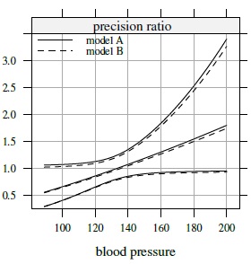
Figure 8.7 Estimates and two-sided 95% simultaneous confidence bands for the precision ratio λ12 under Models A and B.
For agreement evaluation, we compute estimates and one-sided confidence bands for CCC12 and TDI12(0.90) as functions of ![]() . The measures are obtained by setting ψ2 = 0 in (8.30) and (8.31) (Exercise 8.8). Due to the nature of the heteroscedasticity, the CCC function is decreasing in
. The measures are obtained by setting ψ2 = 0 in (8.30) and (8.31) (Exercise 8.8). Due to the nature of the heteroscedasticity, the CCC function is decreasing in ![]() whereas the TDI function is increasing in
whereas the TDI function is increasing in ![]() . In the case of Model B, the measures are adjusted for the effects of the covariates age, gender, and heart rate. They remain a function of gender because of its interaction with method. The estimated CCC ranges from 0.78 to 0.95 for Model A; and from 0.66 to 0.93 and 0.65 to 0.91, respectively, for males and females in the case of Model B. Likewise, the estimated TDI ranges from 10.1 to 23.9 for Model A; and from 9.3 to 24.2 and 10.5 to 24.7, respectively, for males and females in the case of Model B. The methods exhibit higher agreement for males than females because their estimated mean difference is smaller for males. Although gender affects the extent of agreement, its actual effect is quite small because it is tied to the estimated gender × method interaction effect of
. In the case of Model B, the measures are adjusted for the effects of the covariates age, gender, and heart rate. They remain a function of gender because of its interaction with method. The estimated CCC ranges from 0.78 to 0.95 for Model A; and from 0.66 to 0.93 and 0.65 to 0.91, respectively, for males and females in the case of Model B. Likewise, the estimated TDI ranges from 10.1 to 23.9 for Model A; and from 9.3 to 24.2 and 10.5 to 24.7, respectively, for males and females in the case of Model B. The methods exhibit higher agreement for males than females because their estimated mean difference is smaller for males. Although gender affects the extent of agreement, its actual effect is quite small because it is tied to the estimated gender × method interaction effect of ![]() I2 = −2.30 (Table 8.1), which itself is relatively small. The estimated CCC functions under Model B remain below their Model A counterpart. This is due to the fact that the inclusion of covariates leads to a marked reduction in the between-subject variation, which in turn reduces the CCC. In contrast, the estimated TDI functions remain similar under the two models because the covariates have no impact on the precisions of the methods.
I2 = −2.30 (Table 8.1), which itself is relatively small. The estimated CCC functions under Model B remain below their Model A counterpart. This is due to the fact that the inclusion of covariates leads to a marked reduction in the between-subject variation, which in turn reduces the CCC. In contrast, the estimated TDI functions remain similar under the two models because the covariates have no impact on the precisions of the methods.
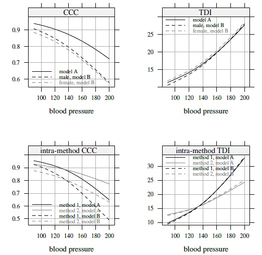
Figure 8.8 One-sided 95% simultaneous confidence bands for TDI(0.90) and CCC—lower bands for CCC and upper bands for TDI—and their intra-method versions for mercury (method 1) and automatic (method 2) methods.
Figure 8.8 presents simultaneous lower confidence bands for CCC and upper confidence bands for TDI under the two models. The covariates affect the bands in the same way as they affect the estimates. The CCC bands range from 0.7 to 0.95 for Model A and from 0.6 to 0.9 for Model B. The extent of agreement between the methods becomes progressively worse as the magnitude of measurement increases. Except possibly near the low end of the measurement range, the methods cannot be deemed to agree well enough to be used interchangeably. For both models, the same conclusion is provided by the TDI bands that increase from 11 to 28 as the blood pressure increases from 89 to 200.
For repeatability evaluation, Figure 8.8 presents simultaneous bands for intra-method CCCj and TDIj(0.90), j = 1, 2. These measures are obtained by setting ψj2 = 0 in (8.39); see Exercise 8.8. The intra-method TDI band ranges from 10 to 35 for the mercury method and from 13 to 25 for the automatic method. The smallest value of 10 implies that, when the true measurement is near 90, two replicate measurements from the same method on the same subject may differ by as much as 10. Relative to the measurement’s magnitude, this difference is too large to be considered acceptable. Therefore, it follows that none of the methods has acceptable repeatability. The same conclusion is reached on the basis of the CCC bands. In fact, when the true measurement is near 200, the mercury method agrees more with the automatic method than with itself on both measures (Exercise 8.8).
To conclude, the two methods under comparison do not agree well despite having similar characteristics. Further, the lack of agreement is driven by poor repeatability of the methods. Although the extent of agreement depends on gender, its actual effect is quite small. The inclusion of subject-level covariates in the model has different consequences for CCC and TDI. The covariates reduce the between-subject variation but have virtually no impact on the error variations of the methods. As a result, the CCC decreases but TDI remains practically unchanged. Thus, the adjusted CCC is smaller than its unadjusted counterpart, thereby making the agreement appear weaker after accounting for covariates. However, no such issue arises with TDI.
8.6 CHAPTER SUMMARY
- The methodologies of previous chapters are generalized to incorporate covariates of two types. The mean covariates affect the means of the methods and the variance covariates affect their variances.
- Covariates are assumed to be fixed, known quantities that are measured without error. They may be continuous or categorical.
- The number of methods may be two or more. They are assumed to have the same scale.
- Measurements may be unreplicated or repeated. In the latter case, they may be unlinked or linked.
- The measures of similarity and agreement do not depend on mean covariates that do not interact with the methods. But they are functions of those that do and also of the variance covariates.
- The measures of repeatability do not depend on mean covariates but depend on variance covariates.
- The agreement measures are adjusted for covariates in the model.
- Inclusion of subject-level mean covariates in the model tends to reduce between-subject variation, which in turn may reduce CCC. The same does not impact TDI unless the covariates interact with the methods or affect their error variations.
- The methodologies for estimating standard errors and constructing confidence intervals are valid only for large number of subjects.
8.7 TECHNICAL DETAILS
This section essentially combines ideas from Sections 6.7 and 7.12 to express the models in Section 8.3.3 in matrix form. Except for the model (8.25) for paired measurements data, all others are mixed-effects models that can be represented in the general form (3.1),
Therefore, it suffices to consider the various design scenarios and identify the terms in this general formulation. Then, the properties such as means, variances, and covariances of measurements obtained in Section 8.3.3 can also be derived using the fact that, under the general formulation, the Yi follow independent ![]() distributions.
distributions.
For the repeated measurements data, define Yi and ei using (7.35), and assume that ei ∼NMi (0, Ri(![]() i)), where
i)), where
Define β and Xi as
 (8.49)
The general representation of model (8.7) for unlinked data from J > 2 methods now follows upon taking Zi and ui given by (7.35). Taking instead Zi and ui given by (7.37) yields the same representation of model (8.15) for linked data from J > 2 methods. These representations hold for models (8.18) and (8.19) for J = 2 as well, provided ![]() in the covariance matrix G of ui is replaced by a common value ψ2. The vector θ of transformed parameters of these models consist of
in the covariance matrix G of ui is replaced by a common value ψ2. The vector θ of transformed parameters of these models consist of ![]() , and additionally, depending upon the model,
, and additionally, depending upon the model, ![]() or log(ψ2), and
or log(ψ2), and ![]() .
.
For unreplicated data from J > 2 methods, the representation for their model (8.20) is obtained by defining Yi, ui, Zi, and ei as in (7.34); taking β as in (8.49); and substituting mij = 1 in (8.48) and (8.49) to get Ri(![]() i) and Xi, respectively. The resulting ui and G are scalar quantities and the matrix Zi = 1J does not depend on the subject index i. The vector θ in this case consists of
i) and Xi, respectively. The resulting ui and G are scalar quantities and the matrix Zi = 1J does not depend on the subject index i. The vector θ in this case consists of ![]() , and δ1,... δJ.
, and δ1,... δJ.
Finally, we consider the paired measurements data Yi =(Yi1, Yi2)T, i = 1,...,n. These vectors follow independent bivariate normal distributions (8.25). The mean vector of this distribution can be written as Xiβ by taking J = 2 and mij = 1 in (8.49). Its covariance matrix is given in (8.25). In this case, ![]() .
.
The models of this chapter are fit by the ML method. For the mixed-effects models, any statistical software capable of fitting such models with heteroscedasticity can be used. For the bivariate normal model, one can use the algorithm described in Section 6.7.2 by modifying it to show that the mean vector µ for subject i is Xiβ and taking the vector θ1 there to be β.
8.8 BIBLIOGRAPHIC NOTE
A number of authors have considered incorporating covariates in the analysis of method comparison data. For paired measurements data, Bland and Altman (1999) use linear regression to model the trend in the Bland-Altman plot as a function of average measurement. The average serves as a proxy for the magnitude of the true measurement. The estimated trend is used to construct the limits of agreement as functions of the average. Geistanger et al. (2008) work with the same setup as Bland and Altman but use nonparametric regression to model the trend.
Barnhart and Williamson (2001) use a generalized estimating equations approach to model CCC as functions of covariates. They also provide a test of equality of CCCs over the covariate values. King and Chinchilli (2001a) develop a stratified CCC that adjusts for categorical covariates and provide a test of homogeneity of CCCs over the strata. Carrasco and Jover (2003) illustrate the importance of adjusting for covariates with a focus on CCC. Their approach involves including covariates in a mixed-effects model for data, but without the method × covariate interactions. They also assume homoscedasticity. Therefore, their CCC adjusted for covariates is a single index free of covariate values. Tsai (2015) recommends model selection to identify important covariates and suggests an estimator of CCC that is a weighted linear combination of the estimators proposed by Barnhart and Williamson (2001) and Carrasco and Jover (2003).
Choudhary and Ng (2006) work with paired measurements data and consider regression modeling of mean and variance of differences as functions of a covariate. Choudhary (2008) works with repeated measurements data and proposes a mixed-effects model that can incorporate covariates and heteroscedasticity. These articles also consider semiparametric modeling of mean functions using penalized splines, but they only focus on TDI as the measure of agreement. The model-based approach of this chapter is motivated by those of Carrasco and Jover (2003) and Choudhary (2008).
Data Source
The blood pressure data are from Carrasco and Jover (2003). They can be obtained from the book’s website.
EXERCISES
- Consider the models (7.1), (7.4), and (7.14) for data on J (≥ 2) methods from Chapter 7. Argue that in each case the mean µj of the marginal distribution of a measurement from method j can be written as µj = βj + µb, j = 1,...,J.
- Consider the model (8.7) for unlinked repeated measurements data from J > 2 methods.
- Verify that the mean and variance of Yijk are given by (8.9) and the covariances are given by (7.6)–(7.7). Verify also that the same expressions are obtained if one uses the model’s matrix representation from Section 8.7.
- Write the companion models for Yj and
 for j = 1,...,J at covariate setting (x1,..., xr, ).
 - Use part (b) to verify that the joint distribution of (Y1,..., YJ) is a J-variate normal distribution with moments given by (8.10). Deduce the distribution (8.11) for the difference Djl.
- Use part (b) to show that for each j = 1,...,J, (Yj, ) follows a bivariate normal distribution with identical univariate normal marginals and covariance given in (8.13). Deduce (8.14).
- This is an analog of Exercise 8.2 for linked data. Consider the model (8.15) for linked repeated measurements data from J > 2 methods.
- Use this model’s matrix representation in Section 8.7 to derive the marginal distribution of data.
- Write the companion models for Yj and for j = 1,..., J at covariate setting (x1,..., xr, ).
- Use part (b) to verify that the joint distribution of (Y1,..., YJ) is J-variate normal with moments given by (8.16). Verify also that the distribution of Djl is given by (8.11).
- Use part (b) to deduce that for each j = 1,..., J, (Yj, ) follows a bivariate normal distribution with identical univariate normal marginals and covariance given in (8.13). Verify (8.17).
- Consider the models (8.18) and (8.19) obtained by taking J = 2 in (8.7) and (8.15), respectively, and setting
 for j = 1, 2. By incorporating the mean function model (8.3) and the variance function model (8.5), show that they generalize, respectively, the models (5.1) and (5.9).
 - Obtain the marginal distribution of the data Yij, j = 1,..., J > 2, i = 1,..., n under the model (8.20) using its matrix representation from Section 8.7. Also, verify the expressions in (8.21)–(8.23).
- Verify the expressions for agreement measures given in Sections 8.4.1 and 8.4.2.
- Verify the expressions for repeatability measures given in Section 8.4.3.
- Consider the blood pressure data from Section 8.5.
- Fit Models A and B and verify the results in Table 8.1.
- Perform model diagnostics for both models. Are the model assumptions reasonable?
- Which model would you prefer? Why?
- Verify the expressions in (8.45)–(8.47).
- Obtain expressions for inter-and intra-method versions of CCC and TDI under Model B and verify the estimates reported in Section 8.5.
- Verify that the mercury method agrees more with the automatic method than with itself when is near 200. What explains this phenomenon?
Consider a study of eggshell thinning in black-headed gulls. The data are available at the book’s website. The study involved ten eggs from each of two stages of development—embryo and feathered. From each egg, three replicate measurements of thickness (µm) were taken in two pigment areas—plain and speckled—at three different locations on the eggshell—blunt, pointy, and equator. Thus, there are 3 × 2 × 3 = 18 observations from each egg, and there is a total of 10 × 2 × 18 = 360 observations in the dataset. The investigators wanted to quantify agreement between the two pigment areas and also to see whether the agreement depends on the stage of development or the eggshell location. In the terminology of this chapter, we can think of this study a method comparison study with eggs as subjects, pigment areas as measurement methods, and stage and location as covariates.
Let Yijkl denote the kth repeated measurement in the jth pigment area of the lth location on the ith egg, l = 1, 2, 3, k = 1, 2, 3, j = 1, 2, i = 1,...,20. Assume that the three repeated measurements are unlinked. Take plain category of pigment area, embryo category of stage, and equator category of location as reference categories.
- Perform an exploratory analysis of data.
- Do stage and location appear to have an effect ? Which interactions appear important?
- Fit the following model to the data:
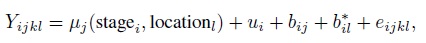
where µj is the mean function of jth pigment area; ui is the random effect of ith egg; bij and
 are random interaction effects between egg and pigment area and location, respectively; and eijkl is the random error term. The random terms are independent for different indices and also independent of each other. Their distributions are as follows:
In the mean function µj (stage, location), include an intercept for jth pigment area, main effects for stage and location, and stage × location interaction effect.
- Evaluate goodness of fit of the assumed model.
- Define Yj and as two replicate measurements of eggshell thickness in the jth pigment area of a given location on an egg of a given stage. Write the companion models for Yj and induced by the assumed model. Find the distributions of (Yj, ), (Y1, Y2), Yj − and Y2 − Y1 at the given stage and location.
- Follow Section 8.4 to derive expressions for measures of similarity between the two pigment areas and also for CCC and TDI for measuring intra-and inter-method agreement between the areas.
- Perform appropriate inference on the measures derived in part (f) to evaluate similarity and repeatability of the two pigment areas and agreement between them. Explain your findings.
- Do the measurements from two pigment areas agree well? Does the extent of agreement depend on either stage or location?