CHAPTER 11
SAMPLE SIZE DETERMINATION
11.1 PREVIEW
This chapter presents a simulation-based methodology to determine sample sizes for planing method comparison studies involving two methods. The focus is on two designs that are most common in practice, namely, the paired measurements design and the repeated measurements designs for unlinked data. For a paired design, we determine the number of subjects that ensure a specified level of precision for estimate of a measure of inter-method agreement. For a repeated measurements design, we determine the number of subjects as well as the number of replications of a measurement that ensure a specified level of precision for estimates of both inter-and intra-method versions of an agreement measure. The methodology is illustrated through an example.
11.2 INTRODUCTION
So far in this book we have focussed on analysis of method comparison data. This chapter considers sample size determination for planning a method comparison study involving two measurement methods. Generally, by “sample size” we mean n—the number of independent subjects in the study. A study with too small a sample size may not be conclusive. On the other extreme, a study with too large a sample size is wasteful. Therefore, statistical considerations are needed to determine a sample size that may be considered adequate.
Two approaches for sample size determination are common. One is designed for the situation when testing hypotheses is the inference of primary interest. In this case, the sample size is determined to ensure that the test with a specified level of significance has a desirable power at a given point in the alternative (research) hypothesis region. The other is designed for the situation when a two-sided confidence interval for a parameter is the inference of primary interest. In this case, the sample size is determined to achieve a specified value for either the width or the expected width of the confidence interval. The former is used if the width is a fixed quantity and the latter is used if the width is a random quantity.
In this book, we have primarily relied on confidence intervals for inference instead of hypotheses testing. Therefore, it is natural for us to adopt a sample size approach based on the confidence intervals. To consider this approach in more detail, note that the width of a two-sided confidence interval is often a constant multiple of the estimated standard error of the estimator used. This is certainly the case here because the 100(1 − α)% confidence interval for a parameter or a parametric function φ is based on a large-sample normal approximation for its estimator ![]() and has the form
and has the form
The standard error used above is estimated from the data. It depends on n, albeit this dependence is suppressed in the notation. From the large sample theory, both the true standard error that SE(![]() ) estimates and the expectation E{SE(
) estimates and the expectation E{SE(![]() )} of this estimator tend to zero as n → ∞. This implies that we can achieve a specified value for the expected width of the interval, 2z1−α/2 E{SE(
)} of this estimator tend to zero as n → ∞. This implies that we can achieve a specified value for the expected width of the interval, 2z1−α/2 E{SE(![]() )}, by taking a sufficiently large sample size.
)}, by taking a sufficiently large sample size.
As this sample size approach for a two-sided confidence interval focuses on the width of the interval, it cannot be directly used for the situation when a one-sided confidence interval of the form

is of primary interest. This is because such intervals have infinite width. However, by turning the focus away from the width of the interval to the standard error of the estimator, the approach can be easily generalized to handle one-sided intervals as well. The general approach determines the sample size that provides a specified value for E{SE(![]() )}. In the case of two-sided intervals, it is equivalent to the one based on the width because the expected width equals the expected standard error times a known constant.
)}. In the case of two-sided intervals, it is equivalent to the one based on the width because the expected width equals the expected standard error times a known constant.
We now consider some issues that come up while adopting this approach for method comparison studies. First, the analysis of method comparison data involves performing inference on a number of measures of similarity and agreement. In this situation, we may determine the sample size required for each measure and take the maximum of the resulting sample sizes. This maximum simultaneously satisfies the requirements for all the measures. However, given that agreement evaluation is the inference of primary interest, it seems appropriate for sample size determination to target only the agreement measures.
Second, herein we use one-sided confidence bounds for two agreement measures, TDI and CCC. The bounds are obtained by first computing them on transformed scales— log(TDI) and z(CCC)—and then applying the corresponding inverse transformations to the results. This means we need to consider standard errors for estimators on the transformed scale and not on the original scale.
Third, the practitioner may choose one of the agreement measures and base sample size computation on that measure. Alternatively, the computation may be done for both the measures and the larger of the two sample sizes may be taken.
Fourth, the expected standard errors do not have closed-form expressions. Therefore, they need to be computed using Monte Carlo simulation.
Finally, sample size determination necessarily depends on the data design and the model assumed for the data. Therefore, these as well as a ballpark value θ0 for the model parameter vector θ also needs to be specified.
We describe the sample size methodology for paired and repeated measurements designs in terms of a general agreement measure φ . These are the two of the most common designs used in method comparison studies. The methodology is illustrated using a case study. Robustness of the methodology with respect to the choice of θ0 is also discussed.
11.3 THE SAMPLE SIZE METHODOLOGY
11.3.1 Paired Measurements Design
Suppose that the data are to be collected using a paired measurements design and they will be modeled using the bivariate normal model (4.6). We need to determine the number of subjects n that would provide an acceptably small value for E{SE(![]() )}. For a given value of n and the ballpark value θ0, the expected standard error is computed as follows:
)}. For a given value of n and the ballpark value θ0, the expected standard error is computed as follows:
This algorithm is used to compute E{SE(![]() )} on a grid of realistic values of n. We can take L = 500 for this computation. The results can be summarized graphically by plotting E{SE(
)} on a grid of realistic values of n. We can take L = 500 for this computation. The results can be summarized graphically by plotting E{SE(![]() )} against n. The practitioner can examine this graph to come up with a level of standard error that is acceptable and take the corresponding n as the desired sample size.
)} against n. The practitioner can examine this graph to come up with a level of standard error that is acceptable and take the corresponding n as the desired sample size.
11.3.2 Repeated Measurements Design
Suppose now that unlinked repeated measurements data are to be collected and they will be modeled using the mixed-effects model (5.1). At the planning stage, it is reasonable to assume that the design is balanced with m replications from each method on every subject. In addition to the number of subjects n, we also need to determine m because it also affects precision of the estimates. For this, however, we restrict attention to m = 2 and 3 because more than 3 replications is rare in practice and is generally not needed (see Section 11.4).
Unlike the paired data, which only allow the evaluation of inter-method agreement, the repeated measurements data additionally allow the evaluation of intra-method agreement—a key objective of method comparison studies (Section 5.6). Therefore, the sample size determination should be targeted towards both the inferences. To this end, let φj denote the intra-method version of φ for jth method, j = 1, 2. We need to determine the number of subjects n and the number of replications m that would provide an acceptably small value for max {E{SE( ![]() )}, E{SE(
)}, E{SE(![]() 1)}, E{SE(
1)}, E{SE(![]() 2)}}. This would imply that all the three standard errors exceed the desired level of accuracy. Presumably, the expected standard errors involved in this criterion are decreasing functions of n. They are also assumed to decrease as m increases from 2 to 3. This assumption needs to be verified.
2)}}. This would imply that all the three standard errors exceed the desired level of accuracy. Presumably, the expected standard errors involved in this criterion are decreasing functions of n. They are also assumed to decrease as m increases from 2 to 3. This assumption needs to be verified.
Just like the paired design case, the expected standard errors for a given (n, m) combination and the ballpark value θ0 can be computed in the following manner:
This algorithm is used to compute the three expected standard errors on a grid of realistic values of n for both m = 2 and 3. We can take L = 500 for this computation. The results can be summarized graphically by plotting them against n separately for m = 2 and 3, possibly on the same graph. The practitioners can examine these results to come up with a level of max{E{SE(![]() )}, E{SE(
)}, E{SE(![]() 1)}, E{SE(
1)}, E{SE(![]() 2)}} that is acceptable and get the corresponding two combinations of (n, m) values. Thereafter, they can calculate the total cost of sampling associated with the options and choose the cheaper one.
2)}} that is acceptable and get the corresponding two combinations of (n, m) values. Thereafter, they can calculate the total cost of sampling associated with the options and choose the cheaper one.
11.4 CASE STUDY
To illustrate the sample size methodology, we need θ0—the ballpark value for the relevant parameter vector θ. For the paired design, this θ represents
the vector of parameters of the bivariate normal model (4.6). For the repeated measurements design, the relevant θ is the vector

of parameters of the mixed-effects model (5.1).
We use estimates obtained from the kiwi data analyzed in Section 5.7.1 to get the θ0. Since these data are unlinked repeated measurements data and are modeled using (5.1), we can directly use the estimates in Table 5.1. This means
 (11.1)
Further, the corresponding values of inter-and intra-method versions of log transformation of TDI(0.90) are

and those of Fisher’s z-transformation of CCC are

For the paired design, we take
 (11.2)
These are parameters of the fitted bivariate normal distribution (5.35) for kiwi data implied by (11.1). It also follows that the underlying values of TDI and CCC and hence their transformations are the same under the two models.
For the illustration, we target sample size determination on the agreement measure TDI. This is primarily because TDI is easier to interpret and, unlike CCC, is not influenced by the between-subject variation in the data. Nevertheless, we also examine the precision of the estimated z(CCC) for the TDI-based sample size.
We begin with sample size determination for a paired design with θ0 given by (11.2). The simulation algorithm from Section 11.3.1 is used with L = 500 to compute the expected standard errors of log {TDI(0.90)} and z(CCC) on a grid of values of n between 30 and 200. The results are presented in Figure 11.1. As anticipated, the expected standard error curves for both measures are decreasing in n. Specifically, the standard error decreases from 0.12 to 0.05 in the case of log {TDI} and from 0.17 to 0.05 in the case of z(CCC).
Suppose the target standard error for log {TDI(0.90)} is 0.06. If we would like to use a 95% upper confidence bound for log {TDI(0.90)}, the standard error of 0.06 implies that the true TDI(0.90) is no more than exp(1.645 × 0.06) = 1.1 times its estimate with 95% confidence (Exercise 11.1). Thus, for example, if the estimated TDI is exp(3.59) = 36.2, the 95% upper confidence bound for the true TDI would be 1.1 × 36.2 = 39.8. Figure 11.1 shows that the target 0.06 for the expected standard error is achieved by n = 125. Therefore, we may take n = 125 as the required sample size. This figure also shows that n = 125 yields 0.085 as the expected standard error for z(CCC). Thus, for example, if the estimated CCC is tanh(1.4) = 0.89, then with this standard error the 95% lower confidence bound for the true CCC would be

Next, we consider sample size determination for a repeated measurements design with θ0 given by (11.1). The simulation algorithm from Section 11.3.2 is used to compute expected standard errors of estimators of inter-and intra-method versions of log{TDI(0.90)} and z(CCC) on the same grid for n as before, separately for m = 2 and 3. Figure 11.2 presents the results. The results for the two intra-method versions of a measure are virtually indistinguishable. Therefore, only those for method 1 are shown. We see that all the expected standard error curves are decreasing in n for a fixed m, and also in m for a fixed n. Further, for both measures, the curve for the intra-method version remains above its counterpart for the inter-method version when m = 2. There is indication that the converse may be true for m = 3; nevertheless, the two curves in this case are quite similar.
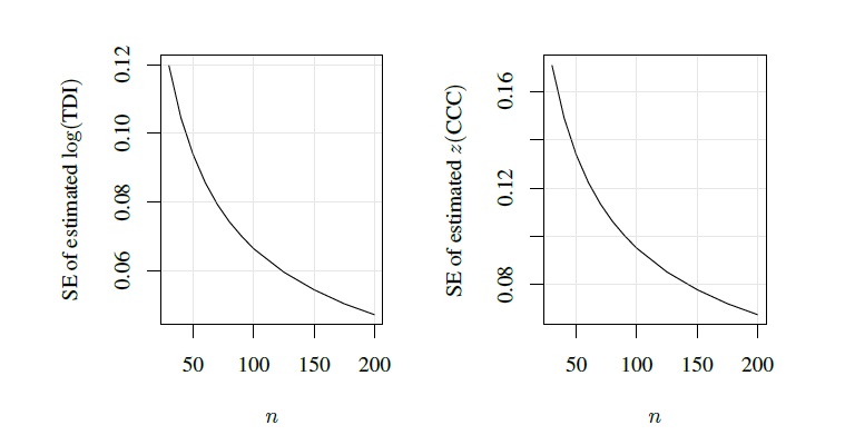
Figure 11.1 Expected standard errors for estimators of log{TDI(0.90)} (left panel) and z(CCC) (right panel) as functions of n for a paired measurements design.
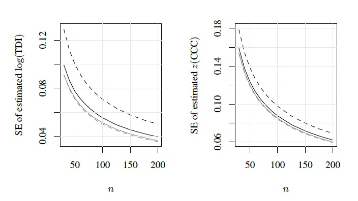
Figure 11.2 Expected standard errors for estimators of inter-and intra-method versions of log{TDI(0.90)} (left panel) and z(CCC) (right panel) as functions of n for a repeated measurements design with m = 2 and 3 replications. In both figures, solid curves are for the inter-method version, with black color for m = 2 and gray for m = 3. The broken curves are for intra-method version for method 1. (Method 2 results are similar and are not shown.)
Table 11.1 Expected standard errors for estimators of various measures.
| (n, m) | log{TDI(0.90)} | log {TDI1(0.90)} | z(CCC) | z(CCC1) |
| (140, 2) | 0.05 | 0.06 | 0.07 | 0.08 |
| (73, 3) | 0.06 | 0.06 | 0.10 | 0.10 |
| (73, 4) | 0.06 | 0.05 | 0.10 | 0.09 |
The target of 0.06 for the maximum of the expected standard errors for estimators of inter-and intra-method versions of log {TDI(0.90)} can be achieved by two (n, m) combinations—(140, 2) and (73, 3). Although a practitioner can now distinguish between the two options by bringing in sampling cost considerations, it seems rather obvious that (73, 3) is likely to be the cheaper option. This is because the cost of taking an additional replication on an existing subject is usually a small fraction of the cost of recruiting an entirely new subject. The maximum over the expected standard errors for the estimated z(CCC) is approximately 0.08 for the (140, 2) combination of (n, m) and is 0.10 for the (73, 3) combination.
These results indicate that there is much gain in increasing m from 2 to 3. It is then natural to wonder whether the same holds when m is increased from 3 to 4. Exercise 11.2 shows that for (n, m) = (73, 4), the expected standard errors, rounded to two decimal places, in the case of inter-and intra-method versions of log {TDI(0.90)} are 0.06 and 0.05, respectively. The corresponding values in the case of z(CCC) are 0.10 and 0.09, respectively. Thus, it is clear that there is little gain in increasing m from 3 to 4 because both (73, 3) and (73, 4) combinations of (n, m) lead to the same value for the maximum expected standard error for the estimators of interest. The actual expected standard errors for these (n, m) combinations are given in Table 11.1.
To examine the robustness of the sample sizes determined above, we repeat the calculation for both paired and repeated measurements designs by making a number of changes to θ0. For the paired design, we set
 (11.3)
where 2208 = exp(7.7) represents the common approximate value for the variances ![]() and
and ![]() reported in (11.2), and take c ∈{0.1, 0.5, 2, 4}. For the repeated measurements design, we set
reported in (11.2), and take c ∈{0.1, 0.5, 2, 4}. For the repeated measurements design, we set
 (11.4)
where σ2 is as defined in (11.3) and varies with c ∈{0.1, 0.5, 2, 4}. From (5.7) and (5.24), these choices imply that the methods have mean zero, their overall variances equal σ2, their correlation equals 0.9, and two measurements from the same method have a correlation of 0.95. Thus, for both paired and repeated measurements designs, we consider 4 parameter settings, with widely different values for σ2, that also differ substantially from the original θ0. It turns out that the results in all cases are practically the same as the ones presented for the original θ0(Exercise 11.2). This shows that the sample sizes are quite robust to the choice of θ0. Essentially, all one needs is a ballpark figure for σ2, the variance of the measurements. As then the sample size determination can proceed by taking the θ0 implied by either (11.3) for the paired measurements design or (11.4) for the repeated measurements design.
Finally, in this book, we have advocated the virtues of replicating measurements by arguing that it allows reliable estimation of error variances, which makes the evaluation of intra-method agreement possible. The above results also show that, even for estimation of measures of inter-method agreement, replicated data require fewer subjects than unreplicated data to achieve the same expected standard error. The reduction may be especially substantial in the case of m = 3. For example, to achieve the target of 0.06 in the case of log {TDI(0.90)}, we need n = 125 for a paired measurements design, whereas only n = 73 is needed for a repeated measurements design with m = 3. Moreover, we have seen that n = 125 for a paired measurements design leads to 0.085 as the expected standard error in the case of z(CCC). The same target is achieved by n = 100 for a repeated measurements design with m = 3. This is another advantage of a repeated measurements design over a paired measurements design.
11.5 CHAPTER SUMMARY
- Sample size can be determined by requiring a desirable precision for the estimate of an agreement measure.
- For a paired measurements design, sample size determination involves computing the number of subjects.
- For a repeated measurements design, sample size determination involves computing the number of subjects as well as the number of replications per subject.
- Generally, more than three replications are not necessary.
- A repeated measurements design may require fewer subjects than a paired measurements design to provide the same precision for estimated measure of inter-method agreement.
- The sample size methodology is quite robust to the choice of the ballpark values for the model parameters under the assumption of bivariate normality.
11.6 BIBLIOGRAPHIC NOTE
Sample size determination for method comparison studies based on power of a hypothesis test involving an agreement measure has been discussed by a number of authors. They include Lin (1992) using CCC, Lin et al. (2002) and Choudhary and Nagaraja (2007) using TDI and CP measures, and Lin et al. (1998) using limits of agreement. See Exercise 12.20 in Chapter 12 for an example of sample size calculation through power analysis. Liao (2009) provides an approach based on notions of discordance rate and tolerance probability. Yin et al. (2008) present a Bayesian approach for sample size determination. Giraudeau and Mary (2001) present a method for computing number of subjects and number of replicates per subject to get a specified expected width of a two-sided confidence interval for an intraclass correlation coefficient.
EXERCISES
- Let
 denote a 100(1 − α)% upper confidence bound for log {TDI(p0)}. For a given value s0 for the standard error, deduce that
Thus, the true TDI(p0) is no more than exp(z1 −αs0) times its estimated value with 100(1 − α)% confidence.
- Verify the various expected standard error estimates reported in Section 11.4 for sample size determination using estimates from the kiwi data given in Table 5.1 on page 129.
- Proceed as in Section 11.4 to perform sample size determination for paired and repeated measurements designs with m = 2 and 3 using estimates obtained from the knee joint angle data presented in Exercise 5.8 on page 138. Assess robustness of the sample sizes to the choice of the ballpark parameter value θ0. How do these sample sizes compare to those reported in Section 11.4?