
Chapter Nine
MATHEMATICAL MODELING USING DIFFERENTIAL EQUATIONS
Contents
9.1 Mathematical Modeling: Setting up a Differential Equation
The Quantity of a Drug in the Body
9.2 Solutions of Differential Equations
Another Look at Marine Harvesting
General Solutions and Particular Solutions
Existence and Uniqueness of Solutions
9.4 Exponential Growth and Decay
Continuously Compounded Interest
The Quantity of a Drug in the Body
The Quantity of a Drug in the Body
Newton's Law of Heating and Cooling
9.6 Modeling the Interaction of Two Populations
A Predator-Prey Model: Robins and Worms
The Slope Field and Equilibrium Points
Trajectories in the wr-Phase Plane
Other Forms of Species Interaction
9.7 Modeling the Spread of a Disease
Flu in a British Boarding School
PROJECTS: Harvesting and Logistic Growth, Population Genetics, The Spread of SARS
9.1 MATHEMATICAL MODELING: SETTING UP A DIFFERENTIAL EQUATION
Sometimes we do not know a function, but we have information about its rate of change, or its derivative. Then we may be able to write a new type of equation, called a differential equation, from which we can get information about the original function. For example, we may use what we know about the derivative of a population function (its rate of change) to predict the population in the future.
In this section, we use a verbal description to write a differential equation.
Marine Harvesting
We begin by investigating the effect of fishing on a fish population. Suppose that, left alone, a fish population increases at a continuous rate of 20% per year. Suppose that fish are also being harvested (caught) by fishermen at a constant rate of 10 million fish per year. How does the fish population change over time?
Notice that we have been given information about the rate of change, or derivative, of the fish population. Combined with information about the initial population, we can use this to predict the population in the future. We know that
![]()
Suppose the fish population, in millions, is P and its derivative is dP/dt, where t is time in years. If left alone, the fish population increases at a continuous rate of 20% per year, so we have
![]()
In addition,
![]()
Since the rate of change of the fish population is dP/dt, we have
![]()
This is a differential equation that models how the fish population changes. The unknown quantity in the equation is the function giving P in terms of t.
Net Worth of a Company
A company earns revenue (income) and also makes payroll payments. Assume that revenue is earned continuously, that payroll payments are made continuously, and that the only factors affecting net worth are revenue and payroll. The company's revenue is earned at a continuous annual rate of 5% times its net worth. At the same time, the company's payroll obligations are paid out at a constant rate of 200 million dollars a year.
We use this information to write a differential equation to model the net worth of the company, W, in millions of dollars, as a function of time, t, in years. We know that
![]()
Since the company's revenue is earned at a rate of 5% of its net worth, we have
![]()
Since payroll payments are made at a rate of 200 million dollars a year, we have
![]()
Putting these two together, since the rate at which net worth is changing is dW/dt, we have
![]()
This is a differential equation that models how the net worth of the company changes. The unknown quantity in the equation is the function giving net worth W as a function of time t.
Pollution in a Lake
If clean water flows into a polluted lake and a stream takes water out, the level of pollution in the lake will decrease (assuming no new pollutants are added).
| Example 1 | The quantity of pollutant in the lake decreases at a rate proportional to the quantity present. Write a differential equation to model the quantity of pollutant in the lake. Is the constant of proportionality positive or negative? Use the differential equation to explain why the graph of the quantity of pollutant against time is decreasing and concave up, as in Figure 9.1.
|
| Solution | Let Q denote the quantity of pollutant present in the lake at time t. The rate of change of Q is proportional to Q, so dQ/dt is proportional to Q. Thus, the differential equation is
Since no new pollutants are being added to the lake, the quantity Q is decreasing over time, so dQ/dt is negative. Thus, the constant of proportionality k is negative. Why does the differential equation dQ/dt = kQ, with k negative, give us the graph shown in Figure 9.1? Since k is negative and Q is positive, we know kQ is negative. Thus, dQ/dt is negative, so the graph of Q against t is decreasing as in Figure 9.1. Why is it concave up? Since Q is getting smaller and k is fixed, as t increases, the product kQ is getting smaller in magnitude, and so the derivative dQ/dt is getting smaller in magnitude. Thus, the graph of Q is more horizontal as t increases. Therefore, the graph is concave up. See Figure 9.1. |

The Quantity of a Drug in the Body
In the previous example, the rate at which pollutants leave a lake is proportional to the quantity of pollutants in the lake. This model works for any contaminants flowing in or out of a fluid system with complete mixing. Another example is the quantity of a drug in a person's body.
The Logistic Model
A population in a confined space grows proportionally to the product of the current population, P, and the difference between the carrying capacity, L, and the current population. (The carrying capacity is the maximum population the environment can sustain.) We use this information to write a differential equation for the population P.
The rate of change of P is proportional to the product of P and L − P, so
![]()
This is called a logistic differential equation. What does it tell us about the graph of P? The derivative dP/dt is the product of k and P and L − P, so when P is small, the derivative dP/dt is small and the population grows slowly. As P increases, the derivative dP/dt increases and the population grows more rapidly. However, as P approaches the carrying capacity L, the term L − P is small, and dP/dt is again small and the population grows more slowly. The logistic growth curve in Figure 9.2 satisfies these conditions.

Figure 9.2: The logistic growth curve is a solution to dP/dt = kP(L − P)
Problems for Section 9.1
1. Match the graphs in Figure 9.3 with the following descriptions.
(a) The temperature of a glass of ice water left on the kitchen table.
(b) The amount of money in an interest-bearing bank account into which $50 is deposited.
(c) The speed of a constantly decelerating car.
(d) The temperature of a piece of steel heated in a furnace and left outside to cool.

2. The graphs in Figure 9.4 represent the temperature, H(°C), of four eggs as a function of time, t, in minutes. Match three of the graphs with the descriptions (a)–(c). Write a similar description for the fourth graph, including an interpretation of any intercepts and asymptotes.
(a) An egg is taken out of the refrigerator (just above 0°C) and put into boiling water.
(b) Twenty minutes after the egg in part (a) is taken out of the fridge and put into boiling water, the same thing is done with another egg.
(c) An egg is taken out of the refrigerator at the same time as the egg in part (a) and left to sit on the kitchen table.

3. A population of insects grows at a rate proportional to the size of the population. Write a differential equation for the size of the population, P, as a function of time, t. Is the constant of proportionality positive or negative?
4. Money in a bank account earns interest at a continuous annual rate of 5% times the current balance. Write a differential equation for the balance, B, in the account as a function of time, t, in years.
5. Radioactive substances decay at a rate proportional to the quantity present. Write a differential equation for the quantity, Q, of a radioactive substance present at time t. Is the constant of proportionality positive or negative?
6. A bank account that initially contains $25,000 earns interest at a continuous rate of 4% per year. Withdrawals are made out of the account at a constant rate of $2000 per year. Write a differential equation for the balance, B, in the account as a function of the number of years, t.
7. A pollutant spilled on the ground decays at a rate of 8% a day. In addition, cleanup crews remove the pollutant at a rate of 30 gallons a day. Write a differential equation for the amount of pollutant, P, in gallons, left after t days.
8. Morphine is administered to a patient intravenously at a rate of 2.5 mg per hour. About 34.7% of the morphine is metabolized and leaves the body each hour. Write a differential equation for the amount of morphine, M, in milligrams, in the body as a function of time, t, in hours.
9. Alcohol is metabolized and excreted from the body at a rate of about one ounce of alcohol every hour. If some alcohol is consumed, write a differential equation for the amount of alcohol, A (in ounces), remaining in the body as a function of t, the number of hours since the alcohol was consumed.
10. Toxins in pesticides can get into the food chain and accumulate in the body. A person consumes 10 micrograms a day of a toxin, ingested throughout the day. The toxin leaves the body at a continuous rate of 3% every day. Write a differential equation for the amount of toxin, A, in micrograms, in the person's body as a function of the number of days, t.
11. A cup of coffee contains about 100 mg of caffeine. Caffeine is metabolized and leaves the body at a continuous rate of about 17% every hour.
(a) Write a differential equation for the amount, A, of caffeine in the body as a function of the number of hours, t, since the coffee was consumed.
(b) Use the differential equation to find dA/dt at the start of the first hour (right after the coffee is consumed). Use your answer to estimate the change in the amount of caffeine during the first hour.
12. A person deposits money into an account at a continuous rate of $6000 a year, and the account earns interest at a continuous rate of 7% per year.
(a) Write a differential equation for the balance in the account, B, in dollars, as a function of years, t.
(b) Use the differential equation to calculate dB/dt if B = 10,000 and if B = 100,000. Interpret your answers.
13. A quantity W satisfies the differential equation
![]()
(a) Is W increasing or decreasing at W = 10? W = 2?
(b) For what values of W is the rate of change of W equal to zero?
14. A quantity y satisfies the differential equation
![]()
Under what conditions is y increasing? Decreasing?
15. An early model of the growth of the Wikipedia assumed that every day a constant number, B, of articles are added by dedicated Wikipedians and that other articles are created by the general public at a rate proportional to the number of articles already there. Express this model as a differential equation for N(t), the total number of Wikipedia articles t days after it started on January 15, 2001.
16. A country's infrastructure is its transportation and communication systems, power plants, and other public institutions. The Solow model asserts that the value of national infrastructure K increases due to investment and decreases due to capital depreciation. The rate of increase due to investment is proportional to national income, Y. The rate of decrease due to depreciation is proportional to the value of existing infrastructure. Write a differential equation for K.
9.2 SOLUTIONS OF DIFFERENTIAL EQUATIONS
What does it mean to “solve” a differential equation? A differential equation is an equation involving the derivative of an unknown function. The unknown is not a number but a function. A solution to a differential equation is any function that satisfies the differential equation.
In this section, we see how to solve a differential equation numerically and how to check whether or not a function is a solution to a differential equation. In the next section, we see how to visualize a solution.
Another Look at Marine Harvesting
Let's take another look at the fish population discussed in Section 9.1. Left alone, the population increases at a continuous rate of 20% per year. The fish are being harvested at a constant rate of 10 million fish per year. If P is the fish population, in millions, in year t, then we have
![]()
Solving this differential equation means finding a function giving P in terms of t. Combined with information about the initial population, we can use the equation to predict the population at any time in the future.
Solving the Differential Equation Numerically
We can approximate the solution to this differential equation by observing that the change in P is approximately dP/dt · Δt when Δt is small.
| Example 1 | Suppose at time t = 0, the fish population is 60 million. Find approximate values for P(t) for t = 1, 2, 3,4, 5. |
| Solution | We can substitute P = 60 into the differential equation to compute the derivative, dP/dt:
Since at t = 0, the fish population is changing at a rate of 2 million fish a year, at the end of the first year, the fish population will have increased by about 2 million fish. So:
We use this new value of P to estimate dP/dt during the second year:
During the second year, the fish population increased by about 2.4 million fish, so:
We use this value of P to estimate the rate of change during the third year, and so on. Continuing in this fashion, we compute the approximate values of P in Table 9.1. This table gives approximate numerical values for P at future times. Table 9.1 Approximate values of the fish population as a function of time
|
A Formula for the Solution to the Differential Equation
A function P = f(t) which satisfies the differential equation
![]()
is called a solution of the differential equation. Table 9.1 shows approximate numerical values of a solution. It is sometimes (but not always) possible to find a formula for the solution. In this particular case, there is a formula; it is
![]()
We check that this is a solution to the differential equation by substituting it into the left and right sides of the differential equation separately. We find

Since we get the same expression on both sides, we say that P = 50 + Ce0.20t is a solution of this differential equation. Any choice of C works, so the solutions form a family of functions with parameter C. Several members of the family of solutions are graphed in Figure 9.5.
Finding the Arbitrary Constant: Initial Conditions
To find a value for the constant C—in other words, to select a single solution from the family of solutions—we need an additional piece of information, usually the initial population. In this case, we know that P = 60 when t = 0, so substituting into
![]()
gives

The function P = 50 + 10e0.20t satisfies the differential equation and the initial condition that P = 60 when t = 0.

Figure 9.5: Solution curves for dP/dt = 0.20P − 10: Members of the family P = 50 + Ce0.20t
General Solutions and Particular Solutions
For the differential equation dP/dt = 0.20P − 10, it can be shown that every solution is of the form P = 50 + Ce0.20t for some value of C. We say that the general solution of the differential equation dP/dt = 0.20P − 10 is the family of functions P = 50 + Ce0.20t. The solution P = 50 + 10e0.20t that satisfies the differential equation together with the initial condition that P = 60 when t = 0 is called a particular solution. The differential equation and the initial condition together are called an initial-value problem.
| Example 2 | (a) Check that P = Ce2t is a solution to the differential equation
(b) Find the particular solution satisfying the initial condition P = 100 when t = 0. |
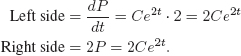
| Solution | (a) Since P = Ce2t where C is a constant, we find expressions for each side:
Since the two expressions are equal, P = Ce2t is a solution to the differential equation. (b) We substitute P = 100 and t = 0 into the general solution P = Ce2t, and solve for C:
The particular solution for this initial-value problem is P = 100e2t. |

| Example 3 | Decide whether or not y = e−2x is a solution of the differential equation y′ − 2y = 0. |
| Solution | Note that y′ = dy/dx. Differentiating y = e−2x gives y′ = −2e−2x. Substituting, we have
and so y = e−2x is not a solution to this differential equation. |
| Example 4 | (a) What conditions must be imposed on the constants C and k if y = Cekt is a solution to the differential equation
(b) What additional conditions must be imposed on C and k if y = Cekt also satisfies the initial condition that y = 10 when t = 0? |
| Solution | (a) If y = Cekt, then dy/dt = Ckekt. Substituting into the equation dy/dt = −0.5y gives
and therefore, assuming C ≠ 0, so Cekt ≠ 0, we have
So y = Ce−0.5t is a solution to the differential equation. If C = 0, then Cekt = 0 is a solution to the differential equation. No conditions are imposed on C. (b) Since k = −0.5, we have y = Ce−0.5t. Substituting y = 10 when t = 0 gives
So y = 10e−0.5t is a solution to the differential equation together with the initial condition. |
Problems for Section 9.2
1. Decide whether or not each of the following is a solution to the differential equation xy′ − 2y = 0.
(a) y = x2
(b) y = x3
2. Check that y = t4 is a solution to the differential equation ![]() .
.
3. Find the general solution to the differential equation
![]()
In Problems 4–12, use the fact that the derivative gives the slope of a curve to decide which of the graphs (A)–(F) in Figure 9.6 could represent a solution to the differential equation.

4. ![]()
5. ![]()
6. ![]()
7. ![]()
8. ![]()
9. ![]()
10. ![]()
11. ![]()
12. ![]()
13. Fill in the missing values in Table 9.2 given that dy/dt = 4 − y. Assume the rate of growth, given by dy/dt, is approximately constant over each unit time interval.
14. Fill in the missing values in Table 9.3 given that dy/dt = 0.5t. Assume the rate of growth, given by dy/dt, is approximately constant over each unit time interval.
15. Fill in the missing values in Table 9.4 given that dy/dt = 0.5y. Assume the rate of growth, given by dy/dt, is approximately constant over each unit time interval.
16. For a certain quantity y, assume that ![]() . Fill in the value of y in Table 9.5. Assume that the rate of growth, dy/dt, is approximately constant over each unit time interval.
. Fill in the value of y in Table 9.5. Assume that the rate of growth, dy/dt, is approximately constant over each unit time interval.
17. If the initial population of fish is 70 million, use the differential equation dP/dt = 0.2P − 10 to estimate the fish population after 1, 2, 3 years.
18. Show that, for any constant P0, the function P = P0et satisfies the equation
![]()
19. Suppose Q = Cekt satisfies the differential equation
![]()
What (if anything) does this tell you about the values of C and k?
20. Is there a value of n which makes y = xn a solution to the equation 13x(dy/dx) = y? If so, what value?
21. Find the values of k for which y = x2 + k is a solution to the differential equation 2y − xy′ = 10.
22. Match solutions and differential equations. (Note: Each equation may have more than one solution, or no solution.)

9.3 SLOPE FIELDS
In this section, we see how to visualize a differential equation and its solutions. Let's start with the equation
![]()
Any solution to this differential equation has the property that at any point in the plane, the slope of its graph is equal to its y coordinate. (That's what the equation dy/dx = y is telling us!) This means that if the solution goes through the point (0, 1), its slope there is 1; if it goes through a point with y = 4 its slope is 4. A solution going through (0, 2) has slope 2 there; at the point where y = 8 the slope of this solution is 8. (See Figure 9.7.)


Figure 9.8: Visualizing the slope of y, if ![]()
In Figure 9.8 a small line segment is drawn at the marked points showing the slope of the solution curve there. Since dy/dx = y, the slope at the point (1, 2) is 2 (the y-coordinate), and so we draw a line segment there with slope 2. We draw a line segment at the point (0, −1) with slope −1, and so on. If we draw many of these line segments, we have the slope field for the equation dy/dx = y shown in Figure 9.9. Above the x-axis, the slopes are positive (because y is positive there), and the slopes increase as we move upward (as y increases). Below the x-axis, the slopes are negative, and get more so as we move downward. Notice that on any horizontal line (where y is constant) the slopes are constant. In the slope field you can see the ghost of the solution curve lurking. Start anywhere on the plane and move so that the slope lines are tangent to your path; you will trace out one of the solution curves. Try penciling in some solution curves on Figure 9.9, some above the x-axis and some below. The curves you draw should have the shape of exponential functions. By substituting y = Cex into the differential equation, you can check that each curve in the family of exponentials, y = Cex, is a solution to this differential equation.

In most problems, we are interested in getting the solution curves from the slope field. Think of the slope field as a set of signposts pointing in the direction you should go at each point. Imagine starting anywhere in the plane: look at the slope field at that point and start to move in that direction. After a small step, look at the slope field again, and alter your direction if necessary. Continue to move across the plane in the direction the slope field points, and you'll trace out a solution curve. Notice that the solution curve is not necessarily the graph of a function, and even if it is, we may not have a formula for the function. Geometrically, solving a differential equation means finding the family of solution curves.
| Example 1 | Figure 9.10 shows the slope field of the differential equation (a) What do you notice about the slope field? (b) Compare the solution curves in Figure 9.11 with the formula y = x2 + C for the solutions to this differential equation.
|
| Solution | (a) In Figure 9.10, notice that on any vertical line (where x is constant) the slopes are all the same. This is because in this differential equation dy/dx depends on x only. (In the previous example, dy/dx = y, the slopes depended on y only.)
(b) The solution curves in Figure 9.11 look like parabolas. It is easy to check by substitution that
so the parabolas y = x2 + C are solution curves; they can also be obtained by using antiderivatives. |


| Example 2 | Using the slope field, guess the equation of the solution curves of the differential equation
|
| Solution | The slope field is shown in Figure 9.12. Notice that on the y-axis, where x is 0, the slope is 0. On the x-axis, where y is 0, the line segments are vertical and the slope is undefined. At the origin the slope is undefined and there is no line segment.
What do the solution curves of this differential equation look like? The slope field suggests they are circles centered at the origin. We guess that the general solution to this differential equation is
This solution is derived in the Focus on Theory section at the end of the chapter.
|

The previous example shows that the solutions to differential equations may sometimes be expressed as implicit functions. Implicit functions are ones which have not been “solved” for y; in other words, the dependent variable is not expressed as an explicit function of x.
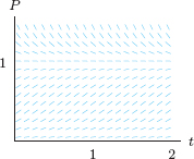
| Example 3 | The slope fields for (a) Which slope field corresponds to which differential equation? (b) Sketch solution curves on each slope field with initial conditions (i) y = 1 when t = 0 (ii) y = 3 when t = 0 (iii) y = 0 when t = 1 (c) For each solution curve, can you say anything about the long-run behavior of y? In particular, as t → ∞, what happens to the value of y?
|
| Solution | (a) Consider the slopes at different points for the two differential equations. In particular, look at the line y = 2 in Figure 9.13. The equation dy/dt = 2 − y has slope 0 all along this line, whereas the line dy/dt = t/2 has slope t/2. Since slope field (I) looks horizontal at y = 2, slope field (I) corresponds to dy/dt = 2 − y and slope field (II) corresponds to dy/dt = t/y.
(b) The initial conditions (i) and (ii) give the value of y when t is 0, that is, the y-intercept. To draw the solution curve satisfying the condition (i), draw the solution curve with y-intercept 1. For (ii), draw the solution curve with y-intercept 3. For (iii), the solution goes through the point (1, 0), so draw the solution curve passing through this point. See Figures 9.14 and 9.15. (c) For dy/dt = 2 − y, all solution curves have y = 2 as a horizontal asymptote, so y → 2 as t → ∞. For dy/dt = t/y with initial conditions (0, 1) and (0, 3), we see that y → ∞ as t → ∞. The graph has asymptotes which appear to be diagonal lines. In fact, they are y = t and y = −t, so y → ±∞ as t → ∞.
Figure 9.14: Solution curves for
|


Existence and Uniqueness of Solutions
Since differential equations are used to model many real situations, the question of whether a solution exists and is unique can have great practical importance. If we know how the velocity of a satellite is changing, can we know its velocity for all future time? If we know the initial population of a city, and we know how the population is changing, can we predict the population in the future? Common sense says yes: if we know the initial value of some quantity and we know exactly how it is changing, we should be able to figure out the future value of the quantity.
In the language of differential equations, an initial-value problem (that is, a differential equation and an initial condition) representing a real situation almost always has a unique solution. One way to see this is by looking at the slope field. Imagine starting at the point representing the initial condition. Through that point there will usually be a line segment pointing in the direction the solution curve must go. By following the line segments in the slope field, we trace out the solution curve. Several examples with different starting points are shown in Figure 9.16. In general, at each point there is one line segment and therefore only one direction for the solution curve to go. Thus the solution curve exists and is unique provided we are given an initial point.
It can be shown that if the slope field is continuous as we move from point to point in the plane, we can be sure that the solution curve exists around every point. Ensuring that each point has only one solution curve through it requires a slightly stronger condition.

Figure 9.16: There is one and only one solution curve through each point in the plane for this slope field
Problems for Section 9.3
1. Sketch three solution curves for each of the slope fields in Figure 9.17.

2. Sketch the slope field for dy/dx = y2 at the points marked in Figure 9.18.


3. Sketch the slope field for dy/dx = x/y at the points marked in Figure 9.19.
4. Figure 9.20 is a slope field for dy/dx = y − 10.
(a) Draw the solution curve for each of the following initial conditions:
(i) y = 8 when x = 0
(ii) y = 12 when x = 0
(iii) y = 10 when x = 0
(b) Since dy/dx = y − 10, when y = 10, we have dy/dx = 10 − 10 = 0. Explain why this matches your answer to part (iii).

Figure 9.20: Slope field for dy/dx = y − 10
5. Figure 9.21 is the slope field for the equation y′ = x + y.
(a) Sketch the solutions that pass through the points
(i) (0, 0)
(ii) (−3, 1)
(iii) (−1, 0)
(b) From your sketch, guess the equation of the solution passing through (−1, 0).
(c) Check your solution to part (b) by substituting it into the differential equation.

Figure 9.21: Slope field for y′ = x + y
6. (a) For dy/dx = x2−y2, find the slope at the following points:
(1, 0), (0, 1), (1, 1), (2, 1), (1, 2), (2, 2)
(b) Sketch the slope field at these points.
7. Match the slope fields in Figure 9.22 with their differential equations:
(a) y′ = 1 + y2
(b) y′ = x
(c) y′ = sin x
(d) y′ = y
(e) y′ = x − y
(f) y′ = 4 − y

Figure 9.22: Each slope field is graphed for −5 ≤ x ≤ 5, −5 ≤ y ≤ 5
8. Match the slope fields in Figure 9.23 with their differential equations. Explain your reasoning.
(a) y′ = −y
(b) y′ = y
(c) y′ = x
(d) y′ = 1/y
(e) y′ = y2

Figure 9.23: Each slope field is graphed for −5 ≤ x ≤ 5, −5 ≤ y ≤ 5
9. Which one of the following differential equations best fits the slope field shown in Figure 9.24? Explain.
I. dP/dt = P − 1
II. dP/dt = P(P − 1)
III. dP/dt = 3P(1 − P)
IV. dP/dt = 1/3P(1−P)
10. (a) Consider the slope field for dy/dx = xy. What is the slope of the line segment at the point (2, 1)? At (0, 2)? At (−1, 1)? At (2, −2)?
(b) Sketch part of the slope field by drawing line segments with the slopes calculated in part (a).
For Problems 11–16, consider a solution curve for each of the slope fields in Problem 7. Write one or two sentences describing qualitatively the long-run behavior of y. For example, as x increases, does y → ∞, or does y remain finite? You may get different limiting behavior for different starting points. In each case, your answer should discuss how the limiting behavior depends on the starting point.
11. Slope field (I)
12. Slope field (IV)
13. Slope field (III)
14. Slope field (V)
15. Slope field (II)
16. Slope field (VI)
17. The Gompertz equation, which models growth of animal tumors, is y′ = −ay ln(y/b), where a and b are positive constants. Use Figures 9.25 and 9.26 to write a paragraph describing the similarities and/or differences between solutions to the Gompertz equation with a = 1 and b = 2 and solutions to the equation y′ = y(2 − y).

Figure 9.25: Slope field for y′ = −y ln(y/2)

Figure 9.26: Slope field for y′ = y(2 − y)
9.4 EXPONENTIAL GROWTH AND DECAY
What is a solution to the differential equation
![]()
A solution is a function that is its own derivative. The function y = et has this property, so y = et is a solution. In fact, any multiple of et also has this property. The family of functions y = Cet is the general solution to this differential equation. If k is a constant, the differential equation
![]()
is similar. This differential equation says that the rate of change of y is proportional to y. The constant k is the constant of proportionality. By substituting y = Cekt into the differential equation, you can check that y = Cekt is a solution. For another derivation of the solution, see the Focus on Theory section at the end of the chapter. We have the following result:
The general solution to the differential equation ![]() is
is
![]()
- This is exponential growth for k > 0, and exponential decay for k < 0.
- The constant C is the value of y when t is 0.
Graphs of solution curves for some k > 0 are in Figure 9.27. For k < 0, the graphs are reflected about the y-axis. See Figure 9.28.
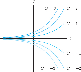
Figure 9.27: Graphs of y = Cekt, which are solutions to ![]() for some fixed k > 0
for some fixed k > 0

Figure 9.28: Graphs of y = Cekt, which are solutions to ![]() for some fixed k < 0
for some fixed k < 0
Population Growth
Consider the population P of a region where there is no immigration or emigration. The rate at which the population is growing is often proportional to the size of the population. This means larger populations grow faster, as we expect since there are more people to have babies. If the population has a continuous growth rate of 2% per unit time, then we know
![]()
so
![]()
This equation is of the form dP/dt = kP for k = 0.02 and has the general solution P = Ce0.02t. If the initial population at time t = 0 is P0, then P0 = Ce0.02(0) = C. So C = P0 and we have
![]()
Continuously Compounded Interest
In Chapter 1 we introduced continuous compounding as the limiting case in which interest was added more and more often. Here we approach continuous compounding from a different point of view. We imagine interest being accrued at a rate proportional to the balance at that moment. Thus, the larger the balance, the faster interest is earned and the faster the balance grows.
| Example 2 | A bank account earns interest continuously at a rate of 5% of the current balance per year. Assume that the initial deposit is $1000 and that no other deposits or withdrawals are made.
(a) Write a differential equation satisfied by the balance in the account. (b) Solve the differential equation and graph the solution. |
| Solution | (a) We are looking for B, the balance in the account in dollars, as a function of t, time in years. Interest is being added continuously to the account at a rate of 5% of the balance at that moment,
so
Thus, a differential equation that describes the process is
Notice that it does not involve the $1000, the initial condition, because the initial deposit does not affect the process by which interest is earned. (b) Since B0 = 1000 is the initial value of B, the solution to this differential equation is
This function is graphed in Figure 9.29.
|

You may wonder how we can represent an amount of money by a differential equation, since money can only take on discrete values (you can't have fractions of a cent). In fact, the differential equation is only an approximation, but for large amounts of money, it is a pretty good approximation.
Pollution in the Great Lakes
In the 1960s pollution in the Great Lakes became an issue of public concern. We will set up a model for how long it would take the lakes to flush themselves clean, assuming no further pollutants were being dumped in the lake.
Let Q be the total quantity of pollutant in a lake of volume V at time t. Suppose that clean water is flowing into the lake at a constant rate r and that water flows out at the same rate. Assume that the pollutant is evenly spread throughout the lake, and that the clean water coming into the lake immediately mixes with the rest of the water.
How does Q vary with time? First, notice that since pollutants are being taken out of the lake but not added, Q decreases, and the water leaving the lake becomes less polluted, so the rate at which the pollutants leave decreases. This tells us that Q is decreasing and concave up. In addition, the pollutants will never be completely removed from the lake though the quantity remaining will become arbitrarily small. In other words, Q is asymptotic to the t-axis. (See Figure 9.30.)
Setting Up a Differential Equation for the Pollution
To understand how Q changes with time, we write a differential equation for Q. We know that
![]()
where the negative sign represents the fact that Q is decreasing. At time t, the concentration of pollutants is Q/V and water containing this concentration is leaving at rate r. Thus,
![]()
So the differential equation is
![]()
and its general solution is
![]()
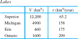
Table 9.6 contains values of r and V for four of the Great Lakes.1 We use this data to calculate how long it would take for certain fractions of the pollution to be removed from Lake Erie.

Figure 9.30: Pollutant in lake versus time
| Example 3 | How long will it take for 90% of the pollution to be removed from Lake Erie? For 99% to be removed? |
| Solution | For Lake Erie, r/V = 175/460 = 0.38, so at time t we have
When 90% of the pollution has been removed, 10% remains, so Q = 0.1Q0. Substituting gives
Canceling Q0 and solving for t gives
Similarly, when 99% of the pollution has been removed, Q = 0.01Q0, so we solve
giving
|
The Quantity of a Drug in the Body
As we saw in Section 9.1, the rate at which a drug leaves a patient's body is proportional to the quantity of the drug left in the body. If we let Q represent the quantity of drug left, then
![]()
The negative sign indicates the quantity of drug in the body is decreasing. The solution to this differential equation is Q = Q0e−kt; the quantity decreases exponentially. The constant k depends on the drug and Q0 is the amount of drug in the body at time zero. Sometimes physicians convey information about the relative decay rate with a half life, which is the time it takes for Q to decrease by a factor of 1/2.
| Example 4 | Valproic acid is a drug used to control epilepsy; its half-life in the human body is about 15 hours.
(a) Use the half-life to find the constant k in the differential equation dQ/dt = −kQ, where Q represents the quantity of drug in the body t hours after the drug is administered. (b) At what time will 10% of the original dose remain? |
| Solution | (a) Since the half-life is 15 hours, we know that the quantity remaining Q = 0.5Q0 when t = 15. We substitute into the solution to the differential equation, Q = Q0e−kt, and solve for k:
(b) To find the time when 10% of the original dose remains in the body, we substitute 0.10Q0 for the quantity remaining, Q, and solve for the time, t.
There will be 10% of the drug still in the body at t = 49.84, or after about 50 hours. |


Problems for Section 9.4
Find solutions to the differential equations in Problems 1–6, subject to the given initial condition.
1. ![]()
2. ![]()
3. ![]()
4. ![]()
5. ![]()
6. ![]()
7. A deposit of $5000 is made to a bank account paying 1.5% annual interest, compounded continuously.
(a) Write a differential equation for the balance in the account, B, as a function of time, t, in years.
(b) Solve the differential equation.
(c) How much money is in the account in 10 years?
8. Money in a bank account grows continuously at an annual rate of r (when the interest rate is 5%, r = 0.05, and so on). Suppose $2000 is put into the account in 2010.
(a) Write a differential equation satisfied by M, the amount of money in the account at time t, measured in years since 2010.
(b) Solve the differential equation.
(c) Sketch the solution until the year 2040 for interest rates of 5% and 10%.
9. A bank account that earns 10% interest compounded continuously has an initial balance of zero. Money is deposited into the account at a continuous rate of $1000 per year.
(a) Write a differential equation that describes the rate of change of the balance B = f(t).
(b) Solve the differential equation.
10. The amount of ozone, Q, in the atmosphere is decreasing at a rate proportional to the amount of ozone present. If time t is measured in years, the constant of proportionality is −0.0025. Write a differential equation for Q as a function of t, and give the general solution for the differential equation. If this rate continues, approximately what percent of the ozone in the atmosphere now will decay in the next 20 years?
11. Using the model in the text and the data in Table 9.6 on page 427, find how long it would take for 90% of the pollution to be removed from Lake Michigan and from Lake Ontario, assuming no new pollutants are added. Explain how you can tell which lake will take longer to be purified just by looking at the data in the table.
12. Use the model in the text and the data in Table 9.6 on page 427 to determine which of the Great Lakes would require the longest time and which would require the shortest time for 80% of the pollution to be removed, assuming no new pollutants are being added. Find the ratio of these two times.
13. The rate at which a drug leaves the bloodstream and passes into the urine is proportional to the quantity of the drug in the blood at that time. If an initial dose of Q0 is injected directly into the blood, 20% is left in the blood after 3 hours.
(a) Write and solve a differential equation for the quantity, Q, of the drug in the blood after t hours.
(b) How much of this drug is in a patient's body after 6 hours if the patient is given 100 mg initially?
14. In some chemical reactions, the rate at which the amount of a substance changes with time is proportional to the amount present. For example, this is the case as δ-glucono-lactone changes into gluconic acid.
(a) Write a differential equation satisfied by y, the quantity of δ-glucono-lactone present at time t.
(b) If 100 grams of δ-glucono-lactone is reduced to 54.9 grams in one hour, how many grams will remain after 10 hours?
15. Oil is pumped continuously from a well at a rate proportional to the amount of oil left in the well. Initially there were 1 million barrels of oil in the well; six years later 500,000 barrels remain.
(a) At what rate was the amount of oil in the well decreasing when there were 600,000 barrels remaining?
(b) When will there be 50,000 barrels remaining?
16. Hydrocodone bitartrate is used as a cough suppressant. After the drug is fully absorbed, the quantity of drug in the body decreases at a rate proportional to the amount left in the body. The half-life of hydrocodone bitartrate in the body is 3.8 hours and the dose is 10 mg.
(a) Write a differential equation for the quantity, Q, of hydrocodone bitartrate in the body at time t, in hours since the drug was fully absorbed.
(b) Solve the differential equation given in part (a).
(c) Use the half-life to find the constant of proportionality, k.
(d) How much of the 10-mg dose is still in the body after 12 hours?
17. The amount of land in use for growing crops increases as the world's population increases. Suppose A(t) represents the total number of hectares of land in use in year t. (A hectare is about 2![]() acres.)
acres.)
(a) Explain why it is plausible that A(t) satisfies the equation A′(t) = kA(t). What assumptions are you making about the world's population and its relation to the amount of land used?
(b) In 1966 about 4.55 billion hectares of land were in use; in 1996 the figure was 4.93 billion hectares.2 If the total amount of land available for growing crops is thought to be 6 billion hectares, when does this model predict it will be exhausted? (Let t = 0 in 1966.)
9.5 APPLICATIONS AND MODELING
In the last section, we considered several situations modeled by the differential equation
![]()
In this section, we consider situations where the rate of change of y is a linear function of y of the form
![]()
The Quantity of a Drug in the Body
A patient is given the drug warfarin, an anticoagulant, intravenously at the rate of 0.5 mg/hour. Warfarin is metabolized and leaves the body at the rate of about 2% per hour. A differential equation for the quantity, Q (in mg), of warfarin in the body after t hours is given by

What does this tell us about the quantity of warfarin in the body for different initial values of Q?
If Q is small, then 0.02Q is also small and the rate the drug is excreted is less than the rate at which the drug is entering the body. Since the rate in is greater than the rate out, the rate of change is positive and the quantity of drug in the body is increasing. If Q is large enough that 0.02Q is greater than 0.5, then 0.5 − 0.02Q is negative, so dQ/dt is negative and the quantity is decreasing.
For small Q, the quantity will increase until the rate in equals the rate out. For large Q, the quantity will decrease until the rate in equals the rate out. What is the value of Q at which the rate in exactly matches the rate out? We have

If the amount of warfarin in the body is initially 25 mg, then the amount being excreted exactly matches the amount being added. The quantity of drug Q will stay constant at 25 mg. Notice also that when Q = 25, the derivative dQ/dt is zero, since
![]()
If the initial quantity is 25, then the solution is the horizontal line Q = 25. This solution is called an equilibrium solution.
The slope field for this differential equation is shown in Figure 9.31, with solution curves drawn for Q0 = 20, Q0 = 25, and Q0 = 30. In each case, we see that the quantity of drug in the body is approaching the equilibrium solution of 25 mg. The solution curve with Q0 = 30 should remind you of an exponential decay function. It is, in fact, an exponential decay function that has been shifted up 25 units.

Figure 9.31: Slope field for dQ/dt = 0.5 − 0.02Q
Solving the Differential Equation dy/dt = k(y − A)
The drug concentration in the previous example satisfies a differential equation of the form
![]()
Let us find the general solution to this equation. Since A is a constant, dA/dt = 0 so that we have
![]()
Thus y − A satisfies an exponential differential equation, so y − A must be of the form
![]()
For an alternative derivation of the solution, see the Focus on Theory section at the end of the chapter.
The general solution to the differential equation
![]()
is
![]()
Warning: Notice that, for differential equations of this form, the arbitrary constant C is not the initial value of the variable, but rather the initial value of y − A.
| Example 2 | At the start of this section, we gave the following differential equation for the quantity of warfarin in the body:
Write the general solution to this differential equation. Find particular solutions for Q0 = 20, Q0 = 25, and Q0 = 30. |
| Solution | We first rewrite the differential equation in the form dQ/dt = k(Q − A) by factoring out −0.02:
The general solution to this differential equation is
To find the particular solution when Q0 = 20, we use the initial condition to solve for C:
The particular solution when Q0 = 20 is Q = 25 − 5e−0.02t. When Q0 = 25, we have C = 0 and the particular solution is the horizontal line Q = 25. When Q0 = 30, we have C = 5 and the particular solution is Q = 25 + 5e−0.02t. These three solutions are the three we saw earlier in Figure 9.31. |
| Example 3 | A company's revenue is earned at a continuous annual rate of 5% of its net worth. At the same time, the company's payroll obligations are paid out at a constant rate of 200 million dollars a year. We saw in Section 9.1 that the differential equation governing the net worth, W (in millions of dollars), of this company in year t is given by
(a) Solve the differential equation, assuming an initial net worth of W0 million dollars. (b) Sketch the solution for W0 = 3000, 4000 and 5000. For which of these values of W0 does the company go bankrupt? In which year? |
| Solution | (a) Factor out 0.05 to get
The general solution is
To find C we use the initial condition that W = W0 when t = 0.
Substituting this value for C into W = 4000 + Ce0.05t gives
(b) If W0 = 4000, then W = 4000, the equilibrium solution. If W0 = 5000, then W = 4000 + 1000e0.05t. If W0 = 3000, then W = 4000 − 1000e0.05t. The graphs of these functions are in Figure 9.32. Notice that if the net worth starts with W0 near, but not equal to, $4000 million, then W moves further away. We see that if W0 = 3000, the value of W goes to 0, and the company goes bankrupt. Solving W = 0 gives t ≈ 27.7, so the company goes bankrupt in its twenty-eighth year.
|


Equilibrium Solutions
Figure 9.31 shows the quantity of warfarin in the body for several different initial quantities. All these curves are solutions to the differential equation
![]()
and all the solutions have the form
![]()
for some C. Notice that Q → 25 as t → ∞ for all solutions because e−0.02t → 0 as t → ∞. In other words, in the long run, the quantity approaches the equilibrium solution of Q = 25 no matter what the initial quantity.
Notice that the equilibrium solution can be found directly from the differential equation by solving dQ/dt = 0:
![]()
giving Q = 25. Because Q always gets closer and closer to the equilibrium value of 25 as t → ∞, we call Q = 25 a stable equilibrium for Q.
A different situation is shown in Figure 9.32 with the solutions to the differential equation dW/dt = 0.05W − 200. We find the equilibrium by looking at the solution curves or by setting dW/dt = 0:
![]()
giving W = 4000 as the equilibrium solution. This equilibrium solution is called unstable because if W starts near, but not equal to, 4000, the net worth W moves further away from 4000 as t → ∞.
- An equilibrium solution is constant for all values of the independent variable. The graph is a horizontal line. Equilibrium solutions can be identified by setting the derivative of the function to zero.
- An equilibrium solution is stable if a small change in the initial conditions gives a solution which tends toward the equilibrium as the independent variable tends to positive infinity.
- An equilibrium solution is unstable if a small change in the initial conditions gives a solution curve which veers away from the equilibrium as the independent variable tends to positive infinity.
In general, a differential equation may have more than one equilibrium solution or no equilibrium solution.
| Example 4 | Find the equilibrium solution for each of the following differential equations. Determine whether the equilibrium solution is stable or unstable.
(a) (b) |
| Solution | (a) To find equilibrium solutions, we set dH/dt = 0:
giving H = 20 as the equilibrium solution. The general solution to this differential equation is H = 20 + Ce−2t. The solution curves for H0 = 10, H0 = 20, and H0 = 30 are shown in Figure 9.33. We see that the equilibrium solution is stable.
Figure 9.33: H = 20 is stable equilibrium
Figure 9.34: B = 10 is unstable equilibrium (b) To find equilibrium solutions, we set dB/dt = 0:
giving B = 10 as the equilibrium solution. The general solution to this differential equation is B = 10 + Ce2t. The solution curves for B0 = 9, B0 = 10, and B0 = 11 are shown in Figure 9.34. We see that the equilibrium solution is unstable. |


Newton's Law of Heating and Cooling
Newton proposed that the temperature of a hot object decreases at a rate proportional to the difference between its temperature and that of its surroundings. Similarly, a cold object heats up at a rate proportional to the temperature difference between the object and its surroundings.
For example, a hot cup of coffee standing on a table cools at a rate proportional to the temperature difference between the coffee and the surrounding air. As the coffee cools, the rate at which it cools decreases because the temperature difference between the coffee and the air decreases. In the long run, the rate of cooling tends to zero and the temperature of the coffee approaches room temperature. Figure 9.35 shows the temperature of two cups of coffee against time, one starting at a higher temperature than the other, but both tending toward room temperature in the long run.

Figure 9.35: Temperature of coffee versus time
Let H be the temperature at time t of a cup of coffee in a 70°F room. Newton's Law says that the rate of change of H is proportional to the temperature difference between the coffee and the room:
![]()
The rate of change of temperature is dH/dt. The temperature difference between the coffee and the room is (H − 70), so
![]()
What about the sign of the constant? If the coffee starts out hotter than 70° (that is, H − 70 > 0), then the temperature of the coffee decreases (i.e., dH/dt < 0) and so the constant must be negative:
![]()
What can we learn from this differential equation? Suppose we take k = 1. The slope field for this differential equation in Figure 9.36 shows several solution curves. Notice that, as we expect, the temperature of the coffee is approaching the temperature of the room. The general solution to this differential equation is
![]()
where C is an arbitrary constant.

| Example 5 | The body of a murder victim is found at noon in a room with a constant temperature of 20°C. At noon the temperature of the body is 35°C; two hours later the temperature of the body is 33°C.
(a) Find the temperature, H, of the body as a function of t, the time in hours since it was found. (b) Graph H against t. What happens to the temperature in the long run? (c) At the time of the murder, the victim's body had the normal body temperature, 37°C. When did the murder occur? |
| Solution | (a) Newton's Law of Cooling says that
Since the temperature difference is H − 20, we have for some constant k
The general solution is
To determine C, we use the fact that H = 35 at t = 0:
So C = 15 and we have
To find k, we use the fact that H = 33 when t = 2:
We isolate the exponential and solve for k:
Therefore, the temperature, H, of the body as a function of time, t, is given by
(b) The graph of H = 20 + 15e−0.072t has a vertical intercept of H = 35, the initial temperature. The temperature decays exponentially with a horizontal asymptote of H = 20. (See Figure 9.37.) “In the long run” means as t → ∞. The graph shows that H → 20 as t → ∞.
Figure 9.37: Temperature of dead body (c) We want to know when the temperature was 37°C. We substitute H = 37 and solve for t:
Taking natural logs on both sides gives
so
The murder occurred about 1.74 hours before noon, that is, about 10:15 am. |


Problems for Section 9.5
Find particular solutions in Problems 1–8.
1. ![]()
2. ![]()
3. ![]()
4. ![]()
5. ![]()
6. ![]()
7. ![]()
8. ![]()
9. Check that y = A + Cekt is a solution to the differential equation
![]()
10. A bank account earns 5% annual interest, compounded continuously. Money is deposited in a continuous cash flow at a rate of $1200 per year into the account.
(a) Write a differential equation that describes the rate at which the balance B = f(t) is changing.
(b) Solve the differential equation given an initial balance B0 = 0.
(c) Find the balance after 5 years.
11. Money in an account earns interest at a continuous rate of 8% per year, and payments are made continuously out of the account at the rate of $5000 a year. The account initially contains $50,000. Write a differential equation for the amount of money in the account, B, in t years. Solve the differential equation. Does the account ever run out of money? If so, when?
12. A company earns 2% per month on its assets, paid continuously, and its expenses are paid out continuously at a rate of $80,000 per month.
(a) Write a differential equation for the value, V, of the company as a function of time, t, in months.
(b) What is the equilibrium solution for the differential equation? What is the significance of this value for the company?
(c) Solve the differential equation found in part (a).
(d) If the company has assets worth $3 million at time t = 0, what are its assets worth one year later?
13. A bank account earns 7% annual interest compounded continuously. You deposit $10,000 in the account, and withdraw money continuously from the account at a rate of $1000 per year.
(a) Write a differential equation for the balance, B, in the account after t years.
(b) What is the equilibrium solution to the differential equation? (This is the amount that must be deposited now for the balance to stay the same over the years.)
(c) Find the solution to the differential equation.
(d) How much is in the account after 5 years?
(e) Graph the solution. What happens to the balance in the long run?
14. One theory on the speed an employee learns a new task claims that the more the employee already knows, the more slowly he or she learns. Suppose that the rate at which a person learns is equal to the percentage of the task not yet learned. If y is the percentage learned by time t, the percentage not yet learned by that time is 100 − y, so we can model this situation with the differential equation
(a) Find the general solution to this differential equation.
(b) Sketch several solutions.
(c) Find the particular solution if the employee starts learning at time t = 0 (so y = 0 when t = 0).
15. A patient is given the drug theophylline intravenously at a rate of 43.2 mg/hour to relieve acute asthma. The rate at which the drug leaves the patient's body is proportional to the quantity there, with proportionality constant 0.082 if time, t, is in hours. The patient's body contains none of the drug initially.
(a) Describe in words how you expect the quantity of theophylline in the patient to vary with time.
(b) Write a differential equation satisfied by the quantity of theophylline in the body, Q(t).
(c) Solve the differential equation and graph the solution. What happens to the quantity in the long run?
16. A chain smoker smokes five cigarettes every hour. From each cigarette, 0.4 mg of nicotine is absorbed into the person's bloodstream. Nicotine leaves the body at a rate proportional to the amount present, with constant of proportionality −0.346 if t is in hours.
(a) Write a differential equation for the level of nicotine in the body, N, in mg, as a function of time, t, in hours.
(b) Solve the differential equation from part (a). Initially there is no nicotine in the blood.
(c) The person wakes up at 7 am and begins smoking. How much nicotine is in the blood when the person goes to sleep at 11 pm (16 hours later)?
17. As you know, when a course ends, students start to forget the material they have learned. One model (called the Ebbinghaus model) assumes that the rate at which a student forgets material is proportional to the difference between the material currently remembered and some positive constant, a.
(a) Let y = f(t) be the fraction of the original material remembered t weeks after the course has ended. Set up a differential equation for y. Your equation will contain two constants; the constant a is less than y for all t.
(b) Solve the differential equation.
(c) Describe the practical meaning (in terms of the amount remembered) of the constants in the solution y = f(t).
18. (a) Find the equilibrium solution of the equation
![]()
(b) Find the general solution of this equation.
(c) Graph several solutions with different initial values.
(d) Is the equilibrium solution stable or unstable?
19. (a) What are the equilibrium solutions for the differential equation
![]()
(b) Use a graphing calculator or computer to sketch a slope field for this differential equation. Use the slope field to determine whether each equilibrium solution is stable or unstable.
20. Figure 9.38 gives the slope field for a differential equation. Estimate all equilibrium solutions and indicate whether each is stable or unstable.

21. A yam is put in a 200°C oven and heats up according to the differential equation
![]()
(a) If the yam is at 20°C when it is put in the oven, solve the differential equation.
(b) Find k using the fact that after 30 minutes the temperature of the yam is 120°C.
22. At 1:00 pm one winter afternoon, there is a power failure at your house in Wisconsin, and your heat does not work without electricity. When the power goes out, it is 68°F in your house. At 10:00 pm, it is 57°F in the house, and you notice that it is 10°F outside.
(a) Assuming that the temperature, T, in your home obeys Newton's Law of Cooling, write the differential equation satisfied by T.
(b) Solve the differential equation to estimate the temperature in the house when you get up at 7:00 am the next morning. Should you worry about your water pipes freezing?
(c) What assumption did you make in part (a) about the temperature outside? Given this (probably incorrect) assumption, would you revise your estimate up or down? Why?
23. A detective finds a murder victim at 9 am. The temperature of the body is measured at 90.3°F. One hour later, the temperature of the body is 89.0°F. The temperature of the room has been maintained at a constant 68°F.
(a) Assuming the temperature, T, of the body obeys Newton's Law of Cooling, write a differential equation for T.
(b) Solve the differential equation to estimate the time the murder occurred.
24. A drug is administered intravenously at a constant rate of r mg/hour and is excreted at a rate proportional to the quantity present, with constant of proportionality α > 0.
(a) Solve a differential equation for the quantity, Q, in milligrams, of the drug in the body at time t hours. Assume there is no drug in the body initially. Your answer will contain r and α. Graph Q against t. What is Q∞, the limiting long-run value of Q?
(b) What effect does doubling r have on Q∞? What effect does doubling r have on the time to reach half the limiting value, ![]() ?
?
(c) What effect does doubling α have on Q∞? On the time to reach ![]() ?
?
25. Some people write the solution of the initial value problem
![]()
in the form
![]()
Show that this formula gives the correct solution for y, assuming y0 ≠ A.
9.6 MODELING THE INTERACTION OF TWO POPULATIONS
So far we have used a differential equation to model the growth of a single quantity. We now consider the growth of two interacting populations, a situation which requires a system of two differential equations. Examples include two species competing for food, one species preying on another, or two species helping each other (symbiosis).
A Predator-Prey Model: Robins and Worms
We model a predator-prey system using what are called the Lotka-Volterra equations. Let's look at a simplified and idealized case in which robins are the predators and worms the prey.3 Suppose there are r thousand robins and w million worms. If there were no robins, the worms would increase exponentially according to the equation
![]()
If there were no worms, the robins would have no food and so their population would decrease according to the equation4
![]()
Now imagine the effect of the two populations on one another. Clearly, the presence of the robins is bad for the worms, so
![]()
On the other hand, the robins do better with the worms around, so
![]()
How exactly do the two populations interact? Let's assume the effect of one population on the other is proportional to the number of “encounters.” (An encounter is when a robin eats a worm.) The number of encounters is likely to be proportional to the product of the populations because if one population is held fixed, the number of encounters should be directly proportional to the other population. So we assume
![]()
where c and k are positive constants.
To analyze this system of equations, let's look at the specific example with a = b = c = k = 1:
![]()
The Phase Plane
To see the growth of the populations, we want graphs of r and w against t. However, it is easier to obtain a graph of r against w first. If we plot a point (w, r) representing the number of worms and robins at any moment, then, as the populations change, the point moves. The wr-plane on which the point moves is called the phase plane and the path of the point is called the phase trajectory.
To find the phase trajectory, we need a differential equation relating w and r directly. We have the two differential equations
![]()
Thinking of r as a function of w and w as a function of t, the chain rule gives
![]()
This tells us that
![]()
so we have
![]()
Figure 9.39 shows the slope field of this differential equation in the phase plane.
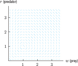
The Slope Field and Equilibrium Points
We can get an idea of what solutions of this equation look like from the slope field. At the point (1, 1) there is no slope drawn because dr/dw is undefined there since the rates of change of both populations with respect to time are zero:
![]()
In terms of worms and robins, this means that if at some moment w = 1 and r = 1 (that is, there are 1 million worms and 1 thousand robins), then w and r remain constant forever. The point w = 1, r = 1 is therefore an equilibrium solution. The origin is also an equilibrium point, since if w = 0 and r = 0, then w and r remain constant. The slope field suggests that there are no other equilibrium points. We check this by solving
![]()
which yields only w = 0, r = 0 and w = 1, r = 1 as solutions.
Trajectories in the wr-Phase Plane
Let's look at the trajectories in the phase plane. A point on a curve represents a pair of populations (w, r) existing at the same time t (though t is not shown on the graph). A short time later, the pair of populations is represented by a nearby point. As time passes, the point traces out a trajectory. It can be shown that the trajectory is a closed curve. See Figure 9.40.
In which direction does the point move on the trajectory? Look at the original pair of differential equations. They tell us how w and r change with time. Imagine, for example, that we are at the point P0 in Figure 9.41, where w = 2.2 and r = 1; then
![]()
Therefore, r is increasing, so the point is moving in the direction shown by the arrow in Figure 9.41.

Figure 9.40: Solution curve is closed

| Example 1 | Suppose that at time t = 0, there are 2.2 million worms and 1 thousand robins. Describe how the robin and worm populations change over time. |
| Solution | The trajectory through the point P0 where w = 2.2 and r = 1 is shown on the slope field in Figure 9.40 and by itself in Figure 9.41.
Initially there are lots of worms so the robin population does well. The robin population is increasing and the worm population is decreasing until there are about 2.2 thousand robins and 1 million worms (point P1 in Figure 9.41). At this point, there are too few worms to sustain the robin population; it begins to decrease and the worm population continues to fall as well. The robin population falls dramatically until there are about 1 thousand robins and 0.4 million worms (point P2 in Figure 9.41). With so few robins, the worm population starts to recover, but the robin population is still decreasing. The worm population increases until there are about 0.4 thousand robins and 1 million worms (P3 in Figure 9.41). Now there are lots of worms for the small population of robins so both populations increase. The populations return to the starting values (since the trajectory forms a closed curve) and the cycle starts over. |
Problem 17 at the end of the section shows how to calculate approximate coordinates of points on the curve.
The Populations as Functions of Time
The shape of a trajectory tells us how the populations vary with time. We use this information to graph each population against time, as in Figure 9.42. The fact that the trajectory is a closed curve means that both populations oscillate periodically. Both populations have the same period, and the worms (the prey) are at their maximum a quarter of a cycle before the robins.

Figure 9.42: Populations of robins (in thousands) and worms (in millions) over time
Lynxes and Hares
A predator-prey system for which there are long-term data is the Canadian lynx and the hare. Both animals were of interest to fur trappers and the records of the Hudson Bay Company shed some light on their populations through much of the 20th century. These records show that both populations oscillated up and down, quite regularly, with a period of about ten years. This is the behavior predicted by Lotka-Volterra equations.
Other Forms of Species Interaction
The methods of this section can be used to model other types of interactions between two species, such as competition and symbiosis.
Problems for Section 9.6
Problems 1–3 give the rates of growth of two populations, x and y, measured in thousands.
(a) Describe in words what happens to the population of each species in the absence of the other.
(b) Describe in words how the species interact with one another. Give reasons why the populations might behave as described by the equations. Suggest species that might interact in that way.
1. ![]()
![]()
2. ![]()
![]()
3. ![]()
![]()
4. The following system of differential equations represents the interaction between two populations, x and y.

(a) Describe how the species interact. How would each species do in the absence of the other? Are they helpful or harmful to each other?
(b) If x = 2 and y = 1, does x increase or decrease? Does y increase or decrease? Justify your answers.
(c) Write a differential equation involving dy/dx.
(d) Use a computer or calculator to draw the slope field for the differential equation in part (c).
(e) Draw the trajectory starting at point x = 2, y = 1 on your slope field, and describe how the populations change as time increases.
Create a system of differential equations to model the situations in Problems 5–7. You may assume that all constants of proportionality are 1.
5. The concentrations of two chemicals are denoted by x and y, respectively. Alone, each decays at a rate proportional to its concentration. Together, they interact to form a third substance. As the third substance is created, the concentrations of the initial two populations get smaller.
6. Two businesses are in competition with each other. Both businesses would do well without the other one, but each hurts the other's business. The values of the two businesses are given by x and y.
7. A population of fleas is represented by x, and a population of dogs is represented by y. The fleas need the dogs in order to survive. The dog population, however, is unaffected by the fleas.
8. Two companies, A and B, are in competition with each other. Let x represent the net worth (in millions of dollars) of Company A, and y represent the net worth (in millions of dollars) of Company B. Four trajectories are given in Figure 9.43. For each trajectory: Describe the initial conditions. Describe what happens initially: Do the companies gain or lose money early on? What happens in the long run?

For Problems 9–19, let w be the number of worms (in millions) and r the number of robins (in thousands) living on an island. Suppose w and r satisfy the following differential equations, which correspond to the slope field in Figure 9.44.
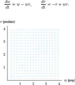
9. Explain why these differential equations are a reasonable model for interaction between the two populations. Why have the signs been chosen this way?
10. Solve these differential equations in the two special cases when there are no robins and when there are no worms living on the island.
11. Describe and explain the symmetry you observe in the slope field. What consequences does this symmetry have for the solution curves?
12. Assume w = 2 and r = 2 when t = 0. Do the numbers of robins and worms increase or decrease at first? What happens in the long run?
13. For the case discussed in Problem 12, estimate the maximum and the minimum values of the robin population. How many worms are there at the time when the robin population reaches its maximum?
14. On the same axes, graph w and r (the worm and the robin populations) against time. Use initial values of 1.5 for w and 1 for r. You may do this without units for t.
15. People on the island like robins so much that they decide to import 200 robins all the way from England, to increase the initial population from r = 2 to r = 2.2 when t = 0. Does this make sense? Why or why not?
16. Assume that w = 3 and r = 1 when t = 0. Do the numbers of robins and worms increase or decrease initially? What happens in the long run?
17. At t = 0 there are 2.2 million worms and 1 thousand robins.
(a) Use the differential equations to calculate the derivatives dw/dt and dr/dt at t = 0.
(b) Use the initial values and your answer to part (a) to estimate the number of robins and worms at t = 0.1.
(c) Using the method of part (a) and (b), estimate the number of robins and worms at t = 0.2 and 0.3.
18. (a) Assume that there are 3 million worms and 2 thousand robins. Locate the point corresponding to this situation on the slope field given in Figure 9.44. Draw the trajectory through this point.
(b) In which direction does the point move along this trajectory? Put an arrow on the trajectory and justify your answer using the differential equations for dr/dt and dw/dt given in this section.
(c) How large does the robin population get? What is the size of the worm population when the robin population is at its largest?
(d) How large does the worm population get? What is the size of the robin population when the worm population is at its largest?
19. Repeat Problem 18 if initially there are 0.5 million worms and 3 thousand robins.
20. For each system of differential equations in Example 2, determine whether x increases or decreases and whether y increases or decreases when x = 2 and y = 2.
For Problems 21–25, suppose x and y are the populations of two different species. Describe in words how each population changes with time.
21.

22.

23.

24.

25. A kidney removes toxin from the blood. If a kidney does not function, the toxin can be removed by dialysis. This problem explores a model for Q1(t), the quantity of toxin in the body outside the blood, and Q2(t), the quantity of toxin in the blood, where t is the time after dialysis started.
(a) The quantity Q1 changes for three reasons. First, toxin is created outside the blood at a constant rate, say A. Second, toxin flows into the blood at a rate proportional to the quantity outside the blood. Third, toxin flows out of the blood at a rate proportional to the quantity in the blood. Write a differential equation for Q1.
(b) The quantity Q2 changes for three reasons. First, dialysis removes toxin from the blood at a rate proportional to the toxin in the blood. Second and third, the same flows into and out of the blood that change Q1 also change Q2. Write a differential equation for Q2.
26. For each system of equations in Example 2, write a differential equation involving dy/dx. Use a computer or calculator to draw the slope field for x, y > 0. Then draw the trajectory through the point x = 3, y = 1.
9.7 MODELING THE SPREAD OF A DISEASE
Differential equations can be used to predict when an outbreak of a disease becomes so severe that it is called an epidemic5 and to decide what level of vaccination is necessary to prevent an epidemic. Let's consider a specific example.
Flu in a British Boarding School
In January 1978, 763 students returned to a boys' boarding school after their winter vacation. A week later, one boy developed the flu, followed immediately by two more. By the end of the month, nearly half the boys were sick. Most of the school had been affected by the time the epidemic was over in mid-February.6
Being able to predict how many people will get sick, and when, is an important step toward controlling an epidemic. This is one of the responsibilities of Britain's Communicable Disease Surveillance Centre and the US's Center for Disease Control and Prevention.
The S-I-R model
We apply one of the most commonly used models for an epidemic, called the S-I-R model, to the boarding school flu example. Imagine the population of the school divided into three groups:
| S = | the number of susceptibles, the people who are not yet sick but who could become sick |
| I = | the number of infecteds, the people who are currently sick |
| R = | the number of recovered, or removed, the people who have been sick and can no longer infect others or be reinfected. |
In this model, the number of susceptibles decreases with time, as people become infected. We assume that the rate people become infected is proportional to the number of contacts between susceptible and infected people. We expect the number of contacts between the two groups to be proportional to both S and I. (If S doubles, we expect the number of contacts to double; similarly, if I doubles, we expect the number of contacts to double.) Thus, we assume that the number of contacts is proportional to the product, SI. In other words, we assume that for some constant a > 0,
![]()
(The negative sign is used because S is decreasing.)
The number of infecteds is changing in two ways: newly sick people are added to the infected group and others are removed. The newly sick people are exactly those people leaving the susceptible group and so accrue at a rate of aSI (with a positive sign this time). People leave the infected group either because they recover (or die), or because they are physically removed from the rest of the group and can no longer infect others. We assume that people are removed at a rate proportional to the number sick, or bI, where b is a positive constant. Thus,
![]()
Assuming that those who have recovered from the disease are no longer susceptible, the recovered group increases at the rate of bI, so
![]()
We are assuming that having the flu confers immunity on a person, that is, that the person cannot get the flu again. (This is true for a given strain of flu, at least in the short run.)
We can use the fact that the total population S+I+R is not changing. (The total population, the total number of boys in the school, did not change during the epidemic; see Problem 2 on page 448.) Thus, once we know S and I, we can calculate R. So we restrict our attention to the two equations

The Constants a and b
The constant a measures how infectious the disease is—that is, how quickly it is transmitted from the infecteds to the susceptibles. In the case of the flu, we know from medical accounts that the epidemic started with one sick boy, with two more becoming sick about a day later. Thus, when I = 1 and S = 762, we have dS/dt ≈ −2, enabling us to roughly7 approximate a:
![]()
The constant b represents the rate at which infected people are removed from the infected population. In this case of the flu, boys were generally taken to the infirmary within one or two days of becoming sick. Assuming half the infected population was removed each day, we take b ≈ 0.5. Thus, our equations are:
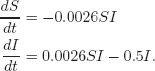
The Phase Plane
As in Section 9.6, we look at trajectories in the phase plane. Thinking of I as a function of S, and S as a function of t, we use the chain rule to get
![]()
so
![]()
Substituting for dI/dt and dS/dt, we get
![]()
Assuming I is not zero, this equation simplifies to approximately
![]()
The slope field of this differential equation is shown in Figure 9.45. The trajectory with initial condition S0 = 762, I0 = 1 is shown in Figure 9.46. Time is represented by the arrow showing the direction that a point moves on the trajectory. The disease starts at the point S0 = 762, I0 = 1. At first, more people become infected and fewer are susceptible. In other words, S decreases and I increases. Later, I decreases as S continues to decrease.

Figure 9.45: Slope field for dI/dS = −1 + 192/S

Figure 9.46: Trajectory for S0 = 762, I0 = 1
What does the SI-Phase Plane Tell Us?
To learn how the disease progresses, look at the shape of the curve in Figure 9.46. The value of I first increases, then decreases to zero. This peak value of I occurs when S ≈ 200. We can determine exactly when the peak value occurs by solving
![]()
which gives
![]()
Notice that the peak value for I always occurs at the same value of S, namely S = 192. The graph shows that if a trajectory starts with S0 > 192, then I first increases and then decreases to zero. On the other hand, if S0 < 192, there is no peak, since I decreases right away.
For this example, the value S =192 is called a threshold population. If S0 is around or below 192, there is no epidemic. If S0 is significantly greater than 192, an epidemic occurs.8
The phase diagram makes clear that the maximum value of I is about 300, which is the maximum number infected at any one time. In addition, the point at which the trajectory crosses the S-axis represents the time when the epidemic has passed (since I = 0). Thus, the S-intercept shows how many boys never get the flu and, hence, how many do get sick.
| Example 1 | In the boarding school model, if S = 400 and I = 250, use Figure 9.46 to decide the signs of dI/dt and dS/dt. Confirm your answers using the differential equations. |
| Solution | Since S = 400 is greater than the peak value of S = 192, we expect that the infected population is still increasing, so dI/dt > 0. The susceptible population is always decreasing (until the disease dies out)), so dS/dt < 0. Checking the differential equations when S = 400 and I = 250, we see dS/dt = −0.0026SI = −260 and dI/dt = 0.0026SI − 0.5I = 135. |
Threshold Value
For the general SIR model, we have the following result:
![]()
If S0, the initial number of susceptibles, is above b/a, there is an epidemic; if S0 is below b/a, there is no epidemic. See Problem 11.
How Many People Should Be Vaccinated?
Faced with an outbreak of the flu or, as happened on several US campuses in the 1980s, of the measles, many institutions consider a vaccination program. How many students must be vaccinated in order to control an outbreak? To answer this, we can think of vaccination as removing people from the S category (without increasing I), which amounts to moving the initial point on the trajectory to the left, parallel to the S-axis. To avoid an epidemic, the initial value of S0 should be around or below the threshold value. Therefore, the boarding-school epidemic would have been avoided if all but 192 students had been vaccinated.
Graphs of S and I Against t
On the trajectory in Figure 9.46, the number of susceptible people decreases throughout the epidemic. This makes sense since people are getting sick and then well again, and thus are no longer susceptible to infection. The trajectory also shows that the number of infected people increases and then decreases. Graphs of S and I against time, t, are shown in Figure 9.47.
To get the scale on the time axis, we would need to use numerical methods. It turns out that the number of infecteds peaked after about 6 days and then dropped. The epidemic ran its course in about 20 days.

Figure 9.47: Progress of the flu over time
Problems for Section 9.7
1. Let I be the number of infected people and S be the number of susceptible people in an outbreak of a disease. Explain why it is reasonable to model the interaction between these two groups by the differential equations

Why have the signs been chosen this way? Why is the constant a the same in both equations?
2. Show that if S, I, and R satisfy the differential equations in Problem 1, the total population, S + I + R, is constant.
3. Explain how you can tell from the graph of the trajectory shown in Figure 9.46 that most people at the British boarding school eventually got sick.
4. (a) In a school of 150 students, one of the students has the flu initially. What is I0? What is S0?
(b) Use these values of I0 and S0 and the equation
![]()
to determine whether the number of infected people initially increases or decreases. What does this tell you about the spread of the disease?
5. Repeat Problem 4 for a school with 350 students.
6. (a) On the slope field for dI/dS in Figure 9.45 trajectory through the point where I = 1 and S = 400.
(b) How many susceptible people are there when the number of infected people is at its maximum?
7. Use Figure 9.47 to estimate the maximum number of infecteds. What does this represent? When does it occur?
8. Compare the diseases modeled by each of the following differential equations with the flu model in this section. Match each set of differential equations with one of the following statements. Write a system of differential equations corresponding to each of the unmatched statements.

(a) More infectious; infecteds removed more slowly.
(b) More infectious; infecteds removed more quickly.
(c) Less infectious; infecteds removed more slowly.
(d) Less infectious; infecteds removed more quickly.
(e) Infecteds never removed.
9. For the equations (I) in Problem 8, what is the threshold value of S?
10. For the equations (II) in Problem 8, suppose S0 = 100. Does the disease spread initially? What if S0 = 200?
11. Let S and I satisfy the differential equations in Problem 1. Assume I ≠ 0.
(a) If dI/dt = 0, find S.
(b) Show that I increases if S is greater than the value you found in part (a). Show that I decreases if S is less than the value you found in part (a).
(c) Explain how you know that your answer to part (a) is the threshold value.
12. During World War I, a particularly lethal form of flu killed about 40 million people around the world.9 The epidemic started in an army camp of 45,000 soldiers outside of Boston, where the first soldier fell sick on September 7, 1918. With time, t, in days since September 7, values of the constants in the SIR model,

are estimated to be a = 0.000267, b = 9.865.
(a) What are the initial values, S0 and I0?
(b) Explain how you know that this model predicts an epidemic in this case.
(c) Find the differential equation for dI/dS. Sketch its slope field and estimate the total number of soldiers infected over the course of the disease.
(d) Solve the differential equation for dI/dS analytically. Use the solution to solve approximately for the number of soldiers affected over the course of the disease.
CHAPTER SUMMARY
- Differential equations terminology
Family of solutions, particular solution, initial conditions, stable/unstable equilibrium solutions
- Estimating values of a solution
- Slope fields
Visualizing the solution to a differential equation
- Solving differential equations analytically
Solutions to dy/dt = ky, and dy/dt = k(y − A)
- Modeling with differential equations
Growth and decay, pollution in a lake, quantity of drug in the body, Newton's law of heating and cooling, net worth of a company
- Systems of differential equations
Interaction of two species or businesses, predator-prey model, spread of a disease
REVIEW PROBLEMS FOR CHAPTER NINE
1. Match the graphs in Figure 9.48 with the following descriptions.
(a) The population of a new species introduced onto a tropical island.
(b) The temperature of a metal ingot placed in a furnace and then removed.
(c) The speed of a car traveling at uniform speed and then braking uniformly.
(d) The mass of carbon-14 in a historical specimen.
(e) The concentration of tree pollen in the air over the course of a year.

2. (a) Determine which of the following functions is a solution to the differential equation
![]()
(i) y = Cx2
(ii) y = Cx3
(iii) y = x3 + C
(b) For any function which is a solution, find C if y = 40 when x = 2.
3. Is y = x3 a solution to the differential equation xy′ − 3y = 0? Justify your answer.
4. For a certain quantity y, assume that dy/dt = −0.20y. Fill in the values of y in Table 9.7. Assume that the rate of growth given by dy/dt is approximately constant over each unit time interval.
5. Slope fields for dy/dx = 1 + x and dy/dx = 1 + y are in Figures 9.49 and 9.50.
(a) Which slope field corresponds to which equation?
(b) On each slope field, draw the solution curve through the origin.
(c) For each slope field, list all equilibrium solutions and indicate whether each is stable or unstable.


6. (a) Sketch the slope field for the equation y′ = x − y in Figure 9.51 at the points indicated.
(b) Check that y = x − 1 is the solution to the differential equation passing through the point (1, 0).

7. Which one of the following differential equations best fits the slope field shown in Figure 9.52? Explain.
I. y′ = 1 + y
II. y′ = 2 − y
III. y′ = (1 + y)(2 − y)
IV. y′ = 1 + x
V. y′ = xy

8. Match each of the slope field segments in (I)–(VI) with one or more of the differential equations in (a)–(f).
(a) y′ = e−x2
(b) y′ = cos y
(c) y′ = cos(4 − y)
(d) y′ = y(4 − y)
(e) y′ = y(3 − y)
(f) y′ = x(3 − x)

9. A deposit is made to a bank account paying an annual interest rate of 7% compounded continuously. No other deposits or withdrawals are made to the account.
(a) Write a differential equation satisfied by B, the balance in the account after t years.
(b) Solve the differential equation given in part (a).
(c) If the initial deposit is $5000, give the particular solution satisfying this initial condition.
(d) How much is in the account after 10 years?
10. Radioactive iodine decays at a continuous rate of about 9% per day. Write a differential equation to model this behavior. Find the general solution.
Solve the differential equations in Problems 11–20.
11. ![]()
12. ![]()
13. ![]()
14. ![]()
15. ![]()
16. ![]()
17. ![]()
18. ![]()
19. ![]()
20. ![]()
21. Write a differential equation whose solution is the temperature as a function of time of a bottle of orange juice taken out of a 40°F refrigerator and left in a 65°F room. Solve the equation and graph the solution.
22. The rate of growth of a tumor is proportional to the size of the tumor.
(a) Write a differential equation satisfied by S, the size of the tumor, in mm, as a function of time, t.
(b) Find the general solution to the differential equation.
(c) If the tumor is 5 mm at time t = 0, what does that tell you about the solution?
(d) If, in addition, the tumor is 8 mm at time t = 3, what does that tell you about the solution?
23. The radioactive isotope carbon-14 is present in small quantities in all life forms, and it is constantly replenished until the organism dies, after which it decays to stable carbon-12 at a rate proportional to the amount of carbon-14 present, with a half-life of 5730 years. Suppose C(t) is the amount of carbon-14 present at time t.
(a) Find the value of the constant k in the differential equation C′ = −kC.
(b) In 1988 three teams of scientists found that the Shroud of Turin, which was reputed to be the burial cloth of Jesus, contained 91% of the amount of carbon-14 contained in freshly made cloth of the same material.10 How old is the Shroud of Turin, according to these data?
24. A bank account earns 5% annual interest compounded continuously. Continuous payments are made out of the account at a rate of $12,000 per year for 20 years.
(a) Write a differential equation describing the balance B = f(t), where t is in years.
(b) Solve the differential equation given an initial balance of B0.
(c) What should the initial balance be such that the account has zero balance after precisely 20 years?
25. Warfarin is a drug used as an anticoagulant. After administration of the drug is stopped, the quantity remaining in a patient's body decreases at a rate proportional to the quantity remaining. The half-life of warfarin in the body is 37 hours.
(a) Sketch the quantity, Q, of warfarin in a patient's body as a function of the time, t, since stopping administration of the drug. Mark the 37 hours on your graph.
(b) Write a differential equation satisfied by Q.
(c) How many days does it take for the drug level in the body to be reduced to 25% of the original level?
26. Dead leaves accumulate on the ground in a forest at a rate of 3 grams per square centimeter per year. At the same time, these leaves decompose at a continuous rate of 75% per year. Write a differential equation for the total quantity of dead leaves (per square centimeter) at time t. Sketch a solution showing that the quantity of dead leaves tends toward an equilibrium level. What is that equilibrium level?
27. Morphine is often used as a pain-relieving drug. The half-life of morphine in the body is 2 hours. Suppose morphine is administered to a patient intravenously at a rate of 2.5 mg per hour, and the rate at which the morphine is eliminated is proportional to the amount present.
(a) Use the half-life to show that, to three decimal places, the constant of proportionality for the rate at which morphine leaves the body (in mg/hour) is k = −0.347.
(b) Write a differential equation for the quantity, Q, of morphine in the blood after t hours.
(c) Use the differential equation to find the equilibrium solution. (This is the long-term amount of morphine in the body, once the system has stabilized.)
28. (a) Find all equilibrium solutions for the equation
![]()
(b) With a calculator or computer, draw a slope field for this differential equation. Use it to determine whether each equilibrium solution is stable or unstable.
29. According to a simple physiological model, an athletic adult male needs 20 Calories per day per pound of body weight to maintain his weight. If he consumes more or fewer Calories than those required to maintain his weight, his weight changes at a rate proportional to the difference between the number of Calories consumed and the number needed to maintain his current weight; the constant of proportionality is 1/3500 pounds per Calorie.
Suppose that a particular person has a constant caloric intake of I Calories per day. Let W(t) be the person's weight in pounds at time t (measured in days).
(a) What differential equation has solution W(t)?
(b) Find the equilibrium solution of the differential equation. Based on the context, do you expect the equilibrium to be stable or unstable?
(c) Solve this differential equation.
(d) Graph W(t) if the person starts out weighing 160 pounds and consumes 3000 Calories a day.
30. (a) Graph f(y) = y − y2.
(b) Sketch the slope field of the differential equation
![]()
(c) Describe how the two graphs are related. In particular, explain how you can determine the equilibrium solutions to the differential equation from the graph of f(y) and how you can tell if the equilibrium solutions are stable.
31. (a) What are the equilibrium solutions to the differential equation y′ = f(y), where f(y) is graphed in Figure 9.53?
(b) Sketch the slope field for y′ = f(y).
(c) For each of the following initial conditions, sketch the solution curve on your slope field:
(i) y(0) = 0
(ii) y(0) = 1
(iii) y(0) = 6
(iv) y(0) = 8
(v) y(0) = 10
(vi) y(0) = 16
(vii) y(0) = 17
(d) Which of the equilibrium solutions are stable? Which are unstable?

STRENGTHEN YOUR UNDERSTANDING
In Problems 1–50, indicate whether the statement is true or false.
1. If a quantity Q is increasing at a constant rate of 8 grams per hour and Q is in grams and t is in hours, then the quantity satisfies the differential equation dQ/dt = 8.
2. If a population P is decreasing at a continuous rate of 5% per year with t in years, then the population satisfies the differential equation dP/dt = −5.
3. If a population P is decreasing at a continuous rate of 5% per year with t in years, then the population satisfies the differential equation dP/dt = 0.05P.
4. If the balance B in a bank account earns 3% interest a year compounded continuously, and there are no other deposits to or withdrawals from the account, then the balance satisfies the differential equation dB/dt = 0.03B, where t is in years.
5. If the rate at which an investment I (in dollars) grows as a function of time t (in years) is proportional to the size of the investment, then dI/dt = kI.
6. If fish in a population are harvested at a rate of 200 tons of fish per year and the fish population would stay stable without the harvesting, then the size of the fish population P in tons satisfies the differential equation dP/dt = −200P where t is in years.
7. If the balance, B, in a bank account is earning interest at a rate of 5 percent per year, compounded continuously, and payments are being made out of the account at a rate of 8000 dollars per year, then the balance B satisfies the differential equation dB/dt = 0.05B − 8000 where B is in dollars and t is in years.
8. If the rate at which the quantity Q of pollutants (in tons) in a lake decreases as a function of time (in years) is proportional to Q, and if new pollutants are being dumped into the lake at a rate of 200 tons per year, then dQ/dt = kQ − 200.
9. If a drug is entering a patient's body through an intravenous line at a continuous rate of 12 mg per hour and if the drug is being metabolized at a continuous rate of 6.3% per hour, then the quantity, Q, in mg, of the drug in the body at time t hours satisfies the differential equation dQ/dt = 12 − 0.063Q.
10. A deposit of $10,000 is made into a bank account and the account earns interest at a rate of 3.2% per year, compounded continuously. The balance, B, in the account in t years satisfies the differential equation dB/dt = 10,000 + 0.032B.
11. The differential equation dP/dt = 3P(10 − P) has P = 10 as a solution.
12. The differential equation dP/dt = 3P(10 − P) has P = 0 as a solution.
13. The differential equation dP/dt = 3P(10 − P) has P = 5 as a solution.
14. If y = Ce0.05t is the general solution to a differential equation, then y = 40e0.05t is the particular solution satisfying the initial condition y(0) = 40.
15. If y = 25 + Ce0.05t is the general solution to a differential equation, then y = 25 + 40e0.05t is the particular solution satisfying the initial condition y(0) = 40.
16. If y = 25 + Ce0.05t is the general solution to a differential equation, then y = 25 + 15e0.05t is the particular solution satisfying the initial condition y(0) = 40.
17. If y(0) = 100 and y′ = 0.2y, then y(1) ≈ 20. Assume the rate of growth is approximately constant over unit intervals.
18. If y(0) = 100 and y′ = 0.2y, then y(1) ≈ 120. Assume the rate of growth is approximately constant over unit intervals.
19. If dQ/dt = 5Q − 200 then when Q = 10, the quantity Q will be decreasing.
20. If dQ/dt = 5Q − 200 there is a solution of the form Q(t) = C for some constant C.
21. The slope field of the differential equation dy/dx = 2x has slope 5 at the point (3, 5).
22. The slope field of the differential equation dy/dx = 2x has slope 6 at the point (3, 5).
23. The slope field of the differential equation dy/dx = 3xy has slope −6 at the point (1, −2).
24. The slope field of the differential equation dy/dx = 3xy has slope 6 at the point (2,2).
25. The slope field of the differential equation dy/dx = 3xy has slope 18 at the point (3, 2).
26. The slope field of the differential equation dy/dx = 2x has positive slopes when y > 0.
27. The slope field of the differential equation dy/dx = 2y has slope 2 at the points (a, 1) for all a.
28. The slope field of the differential equation dy/dx = 5(x–3)(y–2) has horizontal line segments when x = 3.
29. The slope field of the differential equation dP/dt = 12 − 4P has positive slopes when P > 3.
30. The lines in a slope field for a differential equation are tangent to solutions of the differential equation.
31. The general solution of the differential equation dy/dt = ky is y = keCt.
32. The general solution of the differential equation dQ/dt = 0.25Q is Q = Ce0.25t.
33. The general solution of the differential equation dw/dr = 0.3r is w = Ce0.3r.
34. The function H = 57e0.5t is one solution to the differential equation dH/dt = 0.5t.
35. There is exactly one solution of the differential equation dy/dt = 3y which has y(0) = 5.
36. The particular solution of dy/dt = −2y satisfying y = 3 when t = 0 is y = Ce−2t.
37. The balance B in a bank account that earns interest continuously at a rate of 3% per year on an initial deposit of $5000 has differential equation dB/dt = 5000B.
38. If Q(t) is the quantity of a drug in a patient's bloodstream at time t, and the rate at which the drug leaves the bloodstream is proportional to the quantity in the bloodstream, then dQ/dt = −kQ where k is some negative constant.
39. A quantity, Q, of dead leaves decomposes at a rate proportional to the quantity present. We can model this with the differential equation Q = Cekt, where k is negative and t represents time.
40. A quantity, Q, of dead leaves decomposes at a rate proportional to the quantity present. We can model this with the differential equation dQ/dt = kQ, where k is negative and t represents time.
41. The general solution to the differential equation dy/dt = 0.3(y − 75) is y = 75 + Ce0.3t.
42. The general solution to the differential equation dP/dt = 2P − 100 is P = 100 + Ce2t.
43. The general solution to the differential equation dQ/dt = 0.5(Q + 20) is Q = 20 + Ce0.5t.
44. The general solution to the differential equation dW/dt = 600 − 3W is W = 200 + Ce−3t.
45. The solution to the differential equation dA/dt = 0.25(A − 40) with initial condition A(0) = 50 is A = 40 + 50e0.25t.
46. The solution to the differential equation dQ/dt = 50 − 2Q with initial condition Q(0) = 100 is Q = 25 + 75e−2t.
47. The balance, B, in a bank account earns 4% interest per year, compounded continuously, and payments are made out of the account at a rate of $12,000 per year. If t is in years, the differential equation to model this situation is B = 12,000 + Ce0.04t.
48. A drug enters a patient's body intravenously at a continuous rate of 12 mg per hour, and the drug is metabolized at a continuous rate of 18% per hour. If A gives the quantity of drug in the body at hour t, then the differential equation to model this situation is dA/dt = 12 − 0.18A.
49. An equilibrium solution for the differential equation dH/dt = −0.037(H − 225) is H = 225.
50. The graph of an equilibrium solution for a differential equation is a horizontal line.
In Problems 51–60, indicate whether the statement is true or false. Assume x and y represent the sizes of populations of two interacting species X and Y with system of differential equations as given.
51. Assume dx/dt = ax + bxy and dy/dt = cy + dxy. If X would do fine if Y did not exist, then b must be positive.
52. Assume dx/dt = ax + bxy and dy/dt = cy + dxy. If species X eats species Y, then c must be negative.
53. Assume dx/dt = ax + bxy and dy/dt = cy + dxy. If species X eats species Y, then d must be negative.
54. Assume dx/dt = ax + bxy and dy/dt = cy + dxy. If species X cannot survive without species Y and does fine with species Y, then a must be negative and b must be positive.
55. If dx/dt = 0.02x − 0.15xy and dy/dt = 0.05y − 0.18xy, then both populations need the other to survive.
56. If dx/dt = 0.02x − 0.15xy and dy/dt = 0.05y − 0.18xy, then both populations would do fine if the other population did not exist.
57. If dx/dt = 0.02x − 0.15xy and dy/dt = 0.05y − 0.18xy, then the two populations have a negative impact on each other.
58. If dx/dt = −0.12x + 0.07xy and dy/dt = −0.10y + 0.25xy, then the two populations need each other to survive..
59. Assume dx/dt = −3x + xy and dy/dt = 2y −5xy. If x = 1 and y = 2, then both populations will decrease in size.
60. Assume dx/dt = −3x + xy and dy/dt = 2y − 5xy. If x = 2 and y = 5, then both populations will decrease in size.
In Problems 61–70, indicate whether the statement is true or false. The problems refer to the S − I − R model, in which the variable S represents the number of people susceptible to becoming sick, the variable I represents the number of people currently infected, and R represents the rest of the population. We have

61. The derivative dS/dt is negative because people are dying from the epidemic.
62. The parameter a in dS/dt = −aSI is the same as the parameter a in dI/dt = aSI − bI because people are moving from one group to the other.
63. The term −bI in dI/dt = aSI − bI is negative because people are moving back to the susceptible group.
64. The term −bI in dI/dt = aSI − bI is negative because people are either recovering or dying or being separated from the rest of the population and are no longer in either the S group or the I group.
65. If Type I flu is much more contagious than Type II flu, then the parameter b will be larger for Type I flu.
66. If Type I flu is much more contagious than Type II flu, then the parameter a will be larger for Type I flu.
67. If Type I flu lasts 10 days and Type II flu lasts 3 days, then the parameter b will be larger for Type I flu.
68. If Type I flu lasts 10 days and Type II flu lasts 3 days, then the parameter b will be smaller for Type I flu.
69. If a = 0.001 and b = 0.3 and if current numbers are S = 500 and I = 100, then the number of sick people will increase.
70. If a = 0.001 and b = 0.3 and if current numbers are S = 100 and I = 500, then the number of sick people will increase.
PROJECTS FOR CHAPTER NINE
1. Harvesting and Logistic Growth In this project, we look at the effects of harvesting a population which is growing logistically. Harvesting could be, for example, fishing or logging. An important question is what level of harvesting leads to a sustainable yield. In other words, how much can be harvested without having the population depleted in the long run?
(a) When there is no fishing, a population of fish is governed by the differential equation
![]()
where N is the number of fish at time t in years. Sketch a graph of dN/dt against N. Mark on your graph the equilibrium values of N.
Notice on your graph that if N is between 0 and 200, then dN/dt is positive and N increases. If N is greater than 200, then dN/dt is negative and N decreases. Check this by sketching a slope field for this differential equation. Use the slope field to sketch solutions showing N against t for various initial values. Describe what you see.
(b) Fish are now removed by fishermen at a continuous rate of 75 fish/year. Let P be the number of fish at time t with harvesting. Explain why P satisfies the differential equation
![]()
(c) Sketch dP/dt against P. Find and label the intercepts.
(d) Sketch the slope field for the differential equation for P.
(e) Recall that if dP/dt is positive for some values of P, then P increases for these values, and if dP/dt is negative for some values of P, then P decreases for these values. The value of P, however, never goes past an equilibrium value. Use this information and the graph from part (c) to answer the following questions:
(i) What are the equilibrium values of P?
(ii) For what initial values of P does P increase? At what value does P level off?
(iii) For what initial values of P does P decrease?
(f) Use the slope field in part (d) to sketch graphs of P against t, with the initial values:
(i) P(0) = 40
(ii) P(0) = 50
(iii) P(0) = 60
(iv) P(0) = 150
(v) P(0) = 170
(g) Using the graphs you drew, decide what the equilibrium values of the populations are and whether or not they are stable.
(h) We now look at the effect of different levels of fishing on a fish population. If fishing takes place at a continuous rate of H fish/year, the fish population P satisfies the differential equation
![]()
(i) For each of the values H = 75, 100, 200, plot dP/dt against P.
(ii) For which of the three values of H that you considered in part (i) is there an initial condition such that the fish population does not die out eventually?
(iii) Looking at your answer to part (ii), decide for what values of H there is an initial value for P such that the population does not die out eventually.
(iv) Recommend a policy to ensure long-term survival of the fish population.
2. Population Genetics
Population genetics is the study of hereditary traits in a population. A specific hereditary trait has two possibilities, one dominant, such as brown eyes, and one recessive, such as blue eyes11. Let b denote the gene responsible for the recessive trait and B denote the gene responsible for the dominant trait. Each member of the population has a pair of these genes—either BB (dominant individuals), bb (recessive individuals), or Bb (hybrid individuals). The gene frequency of the b gene is the total number of b genes in the population divided by the total number of all genes (b and B) controlling this trait. The gene frequency is essentially constant when there are no mutations or outside influences on the population. In this project, we consider the effect of mutations on the gene frequency.
Let q denote the gene frequency of the b gene. Then q is between 0 and 1 (since it is a fraction of a whole) and, since b and B are the only genes influencing this trait, the gene frequency of the B gene is 1 − q. Let time t be measured in generations. Every generation, a fraction k1 of the b genes mutate to become B genes, and a fraction k2 of the B genes mutate to become b genes.
(a) Explain why the gene frequency q satisfies the differential equation:
![]()
(b) If k1 = 0.0001 and k2 = 0.0004, simplify the differential equation for q and solve it. The initial value is q0. Sketch the solutions with q0 = 0.1 and q0 = 0.9. What is the equilibrium value of q? Explain how you can tell that the gene frequency gets closer to the equilibrium value as generations pass. Explain how you can tell that the equilibrium value is completely determined by the relative mutation rates.
(c) Repeat part (b) if k1 = 0.00003 and k2 = 0.00001.
3. The Spread of SARS
In the spring of 2003, SARS (Severe Acute Respiratory Syndrome) spread rapidly in several Asian countries and Canada. Predicting the course of the disease—how many people would be infected, how long it would last—was important to officials trying to minimize the impact of the disease. This project analyzes the spread of SARS through interaction between infected and susceptible people.
The variables are S, the number of susceptibles, I, the number of infecteds who can infect others, and R, the number removed (this group includes those in quarantine and those who die, as well as those who have recovered and acquired immunity). Time, t, is in days since March 17, 2003, the date the World Health Organization (WHO) started to publish daily SARS reports. On March 17, Hong Kong reported 95 cases. In this model

and S + I + R = 6.8 million, the population of Hong Kong in 2003.12 Estimates based on WHO data give a = 1.25 · 10−8.
(a) What are S0 and I0, the initial values of S and I?
(b) During March 2003, the value of b was about 0.06. Using a calculator or computer, sketch the slope field for this system of differential equations and the solution trajectory corresponding to the initial conditions. (Use 0 ≤ S ≤ 7 · 106, 0 ≤ I ≤ 0.4 · 106.)
(c) What does your graph tell you about the total number of people infected over the course of the disease if b = 0.06? What is the threshold value? What does this value tell you?
(d) During April, as public health officials worked to get the disease under control, people who had been in contact with the disease were quarantined. Explain why quarantining has the effect of raising the value of b.
(e) Using the April value, b = 0.24, sketch the slope field. (Use the same value of a and the same window.)
(f) What is the threshold value for b = 0.24? What does this tell you? Comment on the quarantine policy.
(g) Comment on the effectiveness of each of the following policies intended to prevent an epidemic and protect a city from an outbreak of SARS in a nearby region.
I Close off the city from contact with the infected region. Shut down roads, airports, trains, and other forms of direct contact.
II Institute a quarantine policy. Isolate anyone who has been in contact with a SARS patient or anyone who shows symptoms of SARS.
FOCUS ON THEORY
SEPARATION OF VARIABLES
We have seen how to sketch solution curves of a differential equation using a slope field. Now we see how to solve certain differential equations analytically, finding an equation for the solution curve.
First, we look at a familiar example, the differential equation
![]()
whose solution curves are the circles
![]()
We can check that these circles are solutions by differentiation; the question now is how they were obtained. The method of separation of variables works by putting all the xs on one side of the equation and all the ys on the other, giving
![]()
We then integrate each side separately:
This gives the circles we were expecting:
![]()
You might worry about whether it is legitimate to separate the dx and the dy. The reason it can be done is explained at the end of this section.
The Exponential Growth and Decay Equations
We use separation of variables to derive the general solution of the equation
![]()
Separating variables, we have
![]()
and integrating,
![]()
gives
![]()
Solving for |y| leads to
![]()
where A = eC, so A is positive. Thus,
![]()
where B = ±A, so B is any nonzero constant. Even though there's no C leading to B = 0, we can have B = 0 because y = 0 is a solution to the differential equation. We lost this solution when we divided through by y at the first step. Thus we have derived the solution used earlier in the chapter:
![]()
| Example 1 | Find all solutions of
|
| Solution | We separate variables and integrate:
This gives
where D is a constant of integration. Solving for y leads to
or
Also, C = 0 gives a solution. This is the same result we used earlier. |
| Example 2 | Find and sketch the solution to
|
| Solution | Factoring the right-hand side gives
Separating variables, we get
so
Solving for P leads to
with A = eC, so A > 0. In addition, A = 0 gives a solution. Thus the general solution to the differential equation is
To find the value of B, substitute P = 5 and t = 0 into the general solution, giving
Figure 9.54: Bell-shaped solution curve so
The graph of this function is in Figure 9.54. Since the solution can be rewritten as
the graph has the same shape as the graph of y = e−t2, the bell-shaped curve of statistics. Here the maximum, normally at t = 0, is shifted one unit to the right to t = 1. |

Justification for Separation of Variables
Suppose a differential equation can be written in the form
![]()
Provided f(y) ≠ 0, we write f(y) = 1/h(y) so the right-hand side can be thought of as a fraction,
![]()
If we multiply through by h(y) we get
![]()
Thinking of y as a function of x, so y = y(x), and dy/dx = y′(x), we can rewrite the equation as
![]()
Now integrate both sides with respect to x:
![]()
The form of the integral on the left suggests that we use the substitution y = y(x). Since dy = y′(x) dx, we get
![]()
If we can find antiderivatives of h and g, then this gives the equation of the solution curve.
Note that transforming the original differential equation,
![]()
into
![]()
looks as though we have treated dy/dx as a fraction, cross-multiplied and then integrated. Although that's not exactly what we have done, you may find this a helpful way of remembering the method. In fact, the dy/dx notation was introduced by Leibniz to allow shortcuts like this (more specifically, to make the chain rule look like cancellation).
Problems on Separation of Variables
In Problems 1–12, use separation of variables to find the solutions to the differential equations subject to the given initial conditions.
1. ![]()
2. ![]()
3. ![]()
4. ![]()
5. ![]()
6. ![]()
7. ![]()
8. ![]()
9. ![]()
10. ![]()
11. ![]()
12. ![]()
13. Determine which of the following differential equations are separable. Do not solve the equations.
(a) y′ = y
(b) y′ = x + y
(c) y′ = xy
(d) y′ = sin(x + y)
(e) y′ − xy = 0
(f) y′ = y/x
(g) y′ = ln (xy)
(h) y′ = (sin x)(cos y)
(i) y′ = (sin x)(cos xy)
(j) y′ = x/y
(k) y′ = 2x
(l) y′ = (x+y)/(x+2y)
Use separation of variables to solve the differential equations in Problems 14–19. Assume a, b, and k are nonzero constants.
14. ![]()
15. ![]()
16. ![]()
17. ![]()
18. ![]()
19. ![]()
20. (a) Find the general solution to the differential equation modeling how a person learns:
![]()
(b) Plot the slope field of this differential equation and sketch solutions with y(0) = 25 and y(0) = 110.
(c) For each of the initial conditions in part (b), find the particular solution and add to your sketch.
(d) Which of these two particular solutions could represent how a person learns?
21. (a) Sketch the slope field for the differential equation dy/dx = xy.
(b) Sketch several solution curves.
(c) Solve the differential equation analytically.
1Data from William E. Boyce and Richard C. DiPrima, Elementary Differential Equations (New York: Wiley, 1977).
2http://www.farmingsolutions.org/facts/factscontent_det.asp, accessed June 6, 2011.
3Based on work by Thomas A. McMahon.
4This assumption unrealistically predicts that the robin population will decay exponentially, rather than die out in finite time.
5Exactly when a disease should be called an epidemic is not always clear. The medical profession generally classifies a disease an epidemic when the frequency is higher than usually expected—leaving open the question of what is usually expected. See, for example, Epidemiology in Medicine by C. H. Hennekens and J. Buring (Boston: Little, Brown, 1987).
6Data from the Communicable Disease Surveillance Centre (UK); reported in “Influenza in a Boarding School,” British Medical Journal March 4, 1978, and by J. D. Murray in Mathematical Biology (New York: Springer Verlag, 1990).
7The values of a and b are close to those obtained by J. D. Murray in Mathematical Biology (New York: Springer Verlag, 1990).
8Here we are using J. D. Murray's definition of an epidemic as an outbreak in which the number of infecteds increases from the initial value, I0. See Mathematical Biology (New York: Springer Verlag, 1990).
9“Capturing a Killer Flu Virus,” J. Taukenberger, A. Reid, T. Fanning, in Scientific American, Vol. 292, No. 1, January 2005.
10The New York Times, October 18, 1988.
11Adapted from C. C. Li, Population Genetics (Chicago: University of Chicago Press, 1995).
12www.census.gov, International Data Base (IDB), accessed June 8, 2004.