
6
System Coupling Mechanism and Vehicle Dynamic Model
6.1 Overview of Vehicle Dynamic Model
With the development of automobile technology, the demands for vehicle handling, comfort, safety and other properties have become higher and higher. The corresponding control technology has emerged, and can be seen in the literature[1–6], which relates to vehicle suspension, steering, braking, and other subsystems. Since Segel made a comprehensive summary of vehicle dynamics on ImechE held in 1993[7], entitled “Vehicle ride and handling stability”, vehicle dynamic model has been developed rapidly. With the requirements of improving the overall vehicle performance, the integrated control method has been proposed to achieve this goal.
Many scholars have carried out much research on the modeling of integrated systems. However, the established vehicle dynamics models are mostly a combination of various subsystems. The derived dynamic equations don’t fully reflect the nonlinear coupled relationships and the interrelated effect among the vehicle longitudinal, lateral, and vertical movements. In the actual movements of a moving car, the longitudinal, lateral, and vertical motions are usually coupled tightly, and it is difficult to strictly separate them. In addition, the suspension, braking, and steering control input does not directly control the vehicle longitudinal, lateral, and vertical movements, nor the roll, pitch, and yaw movements although this is done indirectly through the impact of the tyre forces. Therefore, key isues are: the analysis of the braking, steering, suspension, and other chassis subsystem coupling mechanisms; the study of the nonlinear interaction between the tyre and road characteristics; and the establishment of the nonlinearly coupled dynamic models.
6.2 Analysis of the Chassis Coupling Mechanisms
The vehicle chassis is a complex system which includes brakes, steering, suspension and other subsystems. The suspension is a bridge between the body and wheel. The role of the suspension is to transfer the vertical, lateral, and longitudinal forces to the vehicle body. This will have a direct impact on the vehicle ride comfort. The steering system controls the direction of the vehicle and has a direct impact on the steering sensitivity, portability, and handling stability. The role of the braking system is to slow or stop the vehicle motion. The braking safety of a vehicle is determined by its braking performance and directional stability[8].
The suspension, steering, and braking systems determine the vehicle ride comfort, steering portability, handling stability, and driving safety. On the one hand, the movement of individual subsystems has an impact on the performance of the vehicle. However, there is a relationship between the motions of these subsystems. If a subsystem is improved based on individual performance (the design of mechanical structure or the optimization of control parameters), then the simple performance superposition of several subsystems cannot achieve an ideal comprehensive performance of a full vehicle. Therefore, in order to improve vehicle dynamic performance, the coupling relationship between the chassis subsystems must be studied in depth.
There is a strong coupling relationship between the longitudinal dynamics control systems (ABS, TCS, etc.), the lateral dynamics control systems (EPS, AFS and 4WS, etc.), and the vertical dynamics control systems (ASS, SASS, etc.)[9]. The coupling relationship is shown in Figure 6.1.

Figure 6.1 Coupling effects of typical chassis subsystems.
6.2.1 Coupling of Tyre Forces
A car tyre model describes the motion of the tyre, its 6-component forces, and the relationship between its inputs and outputs under specific working conditions. The longitudinal tyre slip ratio, slip angle, radial deformation, camber angle, rotary speed of wheels, and yaw angle determine the output of the models, such as tyre longitudinal force, lateral force, vertical force, roll torque, rolling resistance moment, and aligning torque. There is not only a nonlinear relationship between the inputs and outputs of the tyre model, but also a coupling relationship between the tyres and their 6-component forces.
- The longitudinal force of a tyre is a nonlinear function of the vertical force and longitudinal slip rate. If the longitudinal slip rate increases to a certain value, the longitudinal force decreases slightly. In addition, if the longitudinal slip rate stays unchanged, there is a linear relationship between the longitudinal and vertical forces.
- The lateral force of the tyre is a nonlinear function of the side slip angle and vertical force. If the vertical force is a constant value, there is a linear relationship between the lateral force and slip angle.
- In certain cases of the side slip angle and the vertical force, the tyre lateral force and the longitudinal force influence each other. First, with the increase of the longitudinal slip rate, the tyre longitudinal force increases; if the slip rate reaches a certain value, the longitudinal force gradually decreases and is stabilized[10]. However, the tyre lateral force gradually decreases when the longitudinal slip rate increases; and when the longitudinal slip rate approaches 1, the tyre lateral force is almost 0.
6.2.2 Coupling of the Dynamic Load Distribution
The comprehensive performance of a full vehicle is determined by the external forces. For example, the yaw rate is related to the tyre lateral force, the vertical vibration acceleration of the vehicle body is determined by the vertical force of the sprung mass, and the braking distance is affected by the tyre longitudinal force. Thus, the tyre longitudinal force, lateral force, and sprung mass vertical force are directly or indirectly influenced by the tyre vertical loads. The tyre vertical loads consist of the dynamic and static load. The static load is determined by the vehicle parameters, and the calculation of the dynamic load is affected by the vehicle movements and inertial forces. The coupling of the dynamic load distribution is described as follows.
- When a car is turning, the lateral force is changed as a result of the change of the steering-angle of the front wheel. In addition, the vertical load of the left tyre is not equal to the vertical load of the right tyre, which can affect the steady-state response and even make the car go from an understeer into an oversteer state.
- When a car is steering and braking, the suspension movement will make the front and rear vertical load change, thereby affecting the front and rear longitudinal forces. Furthermore, when the tyre is operating in a saturation state, the increase of the lateral force results in the decrease of the longitudinal force, then the braking distance increases, which reduces the braking safety of the car.
6.2.3 Coupling of Movement Relationship
The vehicle movements are mainly controlled by the accelerator pedal, brake pedal, and steering wheel, and are made up of the longitudinal movement, vertical movement, lateral movement, roll movement, pitch movement, and yaw movement. These movements have a direct or indirect effect on braking, steering and suspension subsystems.
- While a car is steering (or braking), the roll (or pitch) torque affects the sprung mass acceleration, which affects the vehicle ride comfort.
- While a car is steering and braking, the change in the longitudinal and lateral acceleration results in the variation of the longitudinal inertia force and lateral inertia force. Then, a redistribution of the vertical load acting on the wheels occurs, and the lateral force and yaw rate changes, which directly affects the stability and safety of the car.
6.2.4 Coupling of Structure Parameters and Control Parameters
The chassis is a complex system made up of mechanical structures and control systems. There are two methods for designing a traditional chassis system[11].
- The mechanical structure parameters and design objectives are known, the key issue is to choose the appropriate controller and control parameters.
- The controller parameters are known, the design variables are the structure parameters.
The above two methods can be used to obtain a local optimum performance but not a global optimum performance. The reason is the coupling relationship between the mechanical structure system and control system.
In an integrated chassis control system, there is a strong coupling relationship between the control parameters and structural parameters. For example, when designing an active suspension system, first, the mechanical structure parameters (suspension stiffness, damping, sprung mass, etc.), are designed by optimization methods, and then a better static performance is obtained. Second, in order to improve the dynamic performance of the suspension, a controller is designed. However, it is difficult to reach the desired performance requirement, mainly because the internal coupling of the active and passive components is ignored.
6.3 Dynamic Model of the Nonlinear Coupling for the Integrated Controls of a Vehicle[12]
In order to build a nonlinear dynamic model which can reflect each subsystem coupled relationship, a 14-DOF nonlinear coupling dynamic model of a vehicle is built using the Newton-Euler method. Thus, the longitudinal, lateral, vertical, yaw, roll, and pitch movement and the rotation of the wheels are fully reflected[13].
In order to facilitate the derivation of the mathematical models, the following two parallel vehicle coordinate systems are defined.
- The full vehicle coordinate system (xc, yc, zc). The coordinate origin is the centroid position of the vehicle, the xc and yc axes are parallel to the ground, and the zc axis is perpendicular to the ground.
- The sprung mass coordinate system(xs, ys, zs). The coordinate origin is the center of the sprung mass.
In order to build the mathematical model of the full vehicle, the vehicle system is divided into the sprung mass and unsprung mass systems. The simplified model of the vehicle system is shown in Figure 6.2. The relationship between the centers of the vehicle mass and sprung mass is shown in Figure 6.3.

Figure 6.2 Simplified full vehicle system.
Figure 6.3 Relationship between the vehicle centroid and sprung mass centroid.
The position vector of the full vehicle centroid is Rc, the position vector of the sprung mass centroid is rs, and the position vector of the unsprung mass centroid is rui.
The centroid motion of the full vehicle is:
where uc is the longitudinal velocity of the full vehicle centroid, vc is the lateral velocity of the full vehicle centroid, and wc is the vertical velocity of the full vehicle centroid.
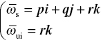
According to the transformation relationship of the coordinate system, the position vector of the sprung mass centroid and the unsprung mass centroid are:

where ρs is the position vector of the sprung mass centroid to the full vehicle mass centroid, ρui is the position vector of the unsprung mass centroid to the full vehicle mass centroid, ![]() are the left front, right front, left rear and right rear wheels, respectively.
are the left front, right front, left rear and right rear wheels, respectively.
From equation (6.2), the absolute velocities of the sprung mass centroid and the unsprung mass centroid are:

where ![]() is the angular velocity of the sprung mass around the centroid axis, and
is the angular velocity of the sprung mass around the centroid axis, and ![]() is the angular velocity of the unsprung mass around the centroid axis.
is the angular velocity of the unsprung mass around the centroid axis.
![]() and
and ![]() can be expressed as follows:
can be expressed as follows:
where p is the roll rate, q is the pitch rate, and r is the yaw rate.
According to Figures 6.2 and 6.3, the position vectors of the sprung mass centroid to the full vehicle mass centroid and the unsprung mass centroid are:

where lF, lR are the distances between the vehicle centroid and the front and rear axles, respectively; hF, hR are the vertical distances from the front and rear sprung mass centroids to the roll axis, respectively; dF, dR are the half front wheel track and the half rear wheel track, respectively; cs is the longitudinal distance from the full vehicle centroid to the sprung mass centroid; and hs is the vertical distance from the full vehicle centroid to the sprung mass centroid.
The absolute velocity vectors of the sprung mass and the unsprung mass are:

The acceleration vectors of the sprung mass and the unsprung mass are:

In order to simplify the calculations, we assume the vehicle longitudinal velocity is constant. According to equation (6.6) and the Newton-Euler method, the differential equations of a vehicle longitudinal, lateral, vertical, roll, yaw, and pitch motion are obtained.
The longitudinal movement of a vehicle is:
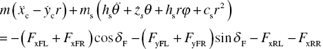
where m is the full vehicle mass, ms is the sprung mass, Fxi is each longitudinal force of the four wheels, Fyi is each lateral force of the four wheels, and δF is the steering-wheel angle.
The lateral movement of a vehicle is:

The vertical movement of a vehicle is:
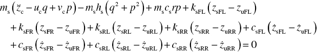
where ksi is the spring stiffness of the four suspensions; csi is the shock absorber damping of the four suspensions; zsi is the vertical displacement of the four sprung masses; and zui is the vertical displacement of the four unsprung masses.
The roll movement of a vehicle is:

where Ixu is the rotary inertia of the sprung mass around the xc axis; Ixzu is the product of inertia of the sprung mass around the xc and zc axes; Iys is the rotary inertia of the sprung mass around the ys axis; Izs is the rotary inertia of the sprung mass around the zs axis; g is the acceleration of gravity; and h is the height of the full vehicle centroid.
The yaw movement of a vehicle is:

where Iz is the rotary inertia of the vehicle around the zc axis, and Ixs is the rotary inertia of the sprung mass around the xs axis.
The pitch movement of a vehicle is:

The vertical movements of the unsprung mass are:

where mui is the unsprung mass, kti is the equivalent spring stiffness of the tyres.
The rotational movements of tyres are:

where Iui is the rotary inertia of the four wheels; ωi is the angular velocity of the four wheels; Ri is the radius of the four wheels; and Tbi is the braking torque of the four wheels, respectively.
The vertical loads of tyres are calculated as[14]:

where Fzi is the vertical load of the four wheels; L is the wheelbase; R0 is the turning radius; h0 is the distance from the vehicle centroid to the roll axis; kφF is the equivalent roll stiffness of the front axle; and kφR is the equivalent roll stiffness of the rear axle.
The slip angles of the tyres are obtained:

6.4 Simulation Analysis
6.4.1 Simulation
In order to verify the results of the analysis of the vehicle dynamics coupling mechanism, according to the nonlinear Magic Formula tyre model described in Chapter 2, the nonlinear coupling dynamic simulation models are built, as shown in Figure 6.4.

Figure 6.4 The simulation models of a nonlinear coupled dynamic system.
The simulation models contain three translational movements along the axes (longitudinal, lateral, and vertical), three rotational movements around the axes (roll, pitch, and yaw), the tyre vertical load calculations, the tyre slip angle calculations, the nonlinear Magic Formula tyre model, and the road input model. The road input model uses a filtered white noise, which is defined as follows[15]:
where G0 is the road roughness coefficient, f0 is the lower cut-off frequency, and w(t) is the Gaussian white noise.
The transfer function between the left and right road input is GRL(s), and the transfer function between the front and rear road input is GFR(s)[12].


where ![]() .
.
The simulation parameters are shown in Table 6.1.
Table 6.1 The vehicle model parameters.
| Parameter | Value | Unit |
| m/ms | 1375/1055 | kg |
| L | 2.4 | m |
| l F/lR | 1.19/1.21 | m |
| c s | 0.15 | m |
| c F/cR | 1.08/1.32 | m |
| h/hs | 0.94/0.1 | m |
| d F/dR | 0.7/0.6 | m |
|
|
40/40/35/35 | kN/m |
|
|
1.4/1.4/1.2/1.2 | kN.s /m |
| I xs/Iys/Izs | 1100/3000/4285 | kg.m2 |
| I xu | 1996 | kg.m2 |
| I xzu | 377.8 | kg.m2 |
| I z/Izx | 5428/47.5 | kg.m2 |
|
|
220/220/220/220 | kN.m−1 |
|
|
12/12/12/12 | kN.m−1 |
|
|
0.25/0.25/0.25/0.25 | m |
| k ϕF/kϕR | 7989/5096 | N/rad |
| f 0 | 0.1 | Hz |
| G 0 | 5×10⁻⁶ | m3/cycle |
6.4.2 Results Analysis
6.4.2.1 Simulation for Vehicle Ride Comfort
- Setting the initial braking speed to 70km/h, the simulation condition studied is emergency braking. The tyre vertical load, the pitch angle of the vehicle body, and the vertical acceleration of vehicle centroid are shown in Figures 6.5–6.7.
- In Figure 6.5, because the vertical loads of the tyres are changed, the front wheel vertical loads increase, and the rear wheel vertical loads are reduced. In Figure 6.6, because of the emergency braking, the pitch angle of the vehicle body increases greatly. In Figure 6.7, the emergency braking not only causes the front and rear axle loads to transfer and the body posture to change, but also causes the vehicle centroid vertical acceleration to increase greatly, which also affects the ride comfort.
The vehicle braking distance curves are shown in Figure 6.8. Because the suspension damper consumes the vehicle vibration energy, the braking distance is reduced in the coupling model.
- In Figure 6.5, because the vertical loads of the tyres are changed, the front wheel vertical loads increase, and the rear wheel vertical loads are reduced. In Figure 6.6, because of the emergency braking, the pitch angle of the vehicle body increases greatly. In Figure 6.7, the emergency braking not only causes the front and rear axle loads to transfer and the body posture to change, but also causes the vehicle centroid vertical acceleration to increase greatly, which also affects the ride comfort.
- Setting the simulation time to 5s, the initial speed of the vehicle to 50km/h, and a step input applied to the steering wheel. The results of the vertical tyre load, lateral acceleration, and roll angle are shown in Figures 6.9–6.11.
- In Figure 6.9, the vertical loads cause a lateral shift. The features seen are that the vertical loads of the inside of the tyres are reduced, while the vertical loads of the outside of the tyres are increased, but the sum of the longitudinal force is constant. However, due to the tyre longitudinal force and lateral force being coupled to each other, the braking distance increases under steering and braking conditions. In Figure 6.10, with the steering peak angle increasing, the body roll angle becomes larger and larger, and the ride comfort deteriorates. In Figure 6.11, with the steering angle increasing, the lateral acceleration becomes larger and larger, and even results in the tyre skidding, so the driving safety is degraded.

Figure 6.5 Vertical load of the tyres during braking.

Figure 6.6 Pitch angle of the vehicle body.

Figure 6.7 Vertical acceleration of the vehicle centroid.

Figure 6.8 Brake distance curves.

Figure 6.9 Vertical loads of the tyres during steering.

Figure 6.10 Roll angles during steering.

Figure 6.11 Lateral acceleration of the vehicle centroid during steering.
6.4.2.2 Simulation for Vehicle Handling Stability
The road surface level is B grade, the initial speed of the vehicle is 70km/h, and a sinusoidal curve is applied to the steering wheel (Figure 6.12). The road adhesion coefficients are 0.9 and 0.5 respectively, and the simulation results are shown in Figures.6.13–6.15.
Figure 6.12 The curve of the steering wheel angle.
Figure 6.13 Yaw rate curves (adhesion coefficient is 0.9).

Figure 6.14 Sideslip angle phase diagram (adhesion coefficient is 0.9).

Figure 6.15 Yaw rate (adhesion coefficient is 0.5).
In Figures 6.13 and 6.14, with the steering angle increasing, the yaw rate and the sideslip angle increase linearly in the linear model. However, the tyre lateral force becomes saturated with the sideslip angle increasing in the nonlinear model, and the deviation between the linear model and the nonlinear model becomes larger and larger.
In Figures 6.15 and 6.16, the yaw rate and sideslip angle of the linear model stay in a linear increasing state, even if the road adhesion coefficient is very low. However, the lateral force of the tyre reaches saturation, an increase of tyre sideslip angle does not make the corresponding lateral force become large, so a driver cannot even control the vehicle in a sudden cornering state; thus, skidding, spin, and other dangerous conditions may occur.

Figure 6.16 Sideslip angle phase diagram (adhesion coefficient is 0.5).
The simulation results show that the nonlinear coupling dynamic models can reflect the coupling relationship among the braking, steering, suspension, and other subsystems. On a low adhesion coefficient road, the yaw rate and sideslip angle obtained from the vehicle dynamic models cannot keep increasing with the increase of the front wheel angle, which can reflect the nonlinear characteristics of the tyres.
References
- [1] Sato Y, Ejiri A, Iida Y, et al. Micro-G emulation system using constant tension suspension for a space manipulator. Proceedings of the IEEE International Conference on Robotics and Automation Sacramento. California, 1991.
- [2] Yao Y S, Mei T. Dynamic modeling and simulation on suspension module. Chinese Journal of Mechanical Engineering, 2006, 42(7): 30–34.
- [3] Liao Y G, Du H I. Modeling and analysis of electric power steering system and its effect on vehicle dynamic behavior. International Journal of Vehicle Autonomous Systems, 2003, 1(3): 351–362.
- [4] Ikenaga S, Lewis F L, Campos J, et al. Active suspension control of ground vehicle based on a full vehicle model. Proceedings of the American Control Conference Chicago, Illinois June, 2000.
- [5] Lee B R, Sin K H. Slip-ration control of ABS using sliding mode control. School of Mechanical and Automotive Engineering University of Ulsan, 1993, 1(2):72–77.
- [6] Segawa M, Nakano S, Nishibara O, et al. Vehicle stability control strategy for steer by wire system. JSAE Review, 2001, 22(4): 383–388.
- [7] Segel L. An overview of developments in road vehicle dynamics: Past, present and future. Proceedings of Imech E Conference on Vehicle Ride and Handling, 1993.
- [8] Chen J R. Automobile Structure. Beijing: Machinery Industry Press, 2000.
- [9] Lu S B. Study on Vehicle Chassis Key Subsystems and its Integrated Control Strategy. PhD Thesis, Chongqing: Chongqing University, 2009.
- [10] Wang Q D, Wang X, Chen W W. Coordination control of active front wheel steering and ABS. Agricultural Machinery Journal, 2008, 39(3): 1–4.
- [11] Wang Q D, Jiang W H, et al. Simultaneous optimization of mechanical and control parameters for integrated control system of active suspension and electric power steering. Chinese Journal of Mechanical Engineering, 2008, 44(8): 67–72.
- [12] Zhu M F. Research on Decoupling Control Method of Vehicle Chassis and Time-delay Control of Chassis Key Subsystems. PhD Thesis, Hefei University of Technology, Hefei, 2011.
- [13] Cui S M, Xiao L S, et al. A research on computer simulation for vehicle handling dynamics with 18 DOFs. Automotive Engineering, 1998, 20(4): 212–219.
- [14] Zhu H. Vehicle Chassis Integrated Control Based on Magneto-rheological Semi-active Suspension. PhD Thesis, Hefei: Hefei University of Technology, 2009.
- [15] Yu F, Lin Y. Automotive System Dynamics. Beijing: Machinery Industry Press, 2008.