
Chapter 14: Spatiotemporal Dynamics and Light Bullets in Nematic Liquid Crystals
Institute for Complex Systems, ISC-CNR, Rome, Italy
We see only what we know.
Johann Wolfgang von Goethe (1749–1832)
14.1 Introduction
Electromagnetic wave packets tend to spread out as they evolve, whatever dimension (time or space) is involved. The fundamental cause of this phenomenon is the propagation at different velocities or directions of the wave packet frequency components. Hence, similar to the beam diffracting in space, pulses spread in time because of the so-called group-velocity-dispersion (GVD), as the energy associated to the various Fourier components of the field tends to temporally shift in propagation. One of the most challenging goals in the study of multidimensional nonlinear field–matter interactions is the generation of wave packets confined in both time and space or light bullets. This term was coined in 1990 by Silberberg [1] to stress the particle nature of such nonlinear objects. We refer to these self-confined waves, or spatiotemporal solitons (STSs), as (2 + 1 + 1)D solitary waves, where the “2” refers to the confinement along the two transverse spatial dimensions, the former “1” relates to the confinement in the time coordinate and the latter “1” refers to the spatial propagation direction.
The formation of STSs requires the simultaneous nonlinear compensation of GVD and diffraction, respectively, occurring in the (1 + 1)D temporal and (2 + 1)D spatial counterparts. Indeed, the number of dimensions in which the nonlinear dynamics evolve is a central issue in the soliton stability as it determines the strength of the nonlinear focusing in the competitive action with the linear diffraction and dispersion [2]. The general nematicon phenomenology is an interesting example of the general stability problem arising as dimensionality of the nonlinear propagation increases.
In a simple picture (as explained in the previous chapters), mechanisms such as saturations [3, 4], absorption [5–7], and the nonlocality [8, 9] can introduce higher-order terms in the nonlinear response, stabilizing the otherwise unstable (2 + 1)D Kerr solitary wave [10, 11].
The current investigation on (2 + 1 + 1)D optical bullets is then facing two major challenges: (i) the formalization of relevant models predicting the stable propagation of STS and (ii) the identification of suitable optical media or systems where such models apply. A number of specific nonlinear regimes are known to theoretically allow STS. For example, conditions for stable STS propagation have been theoretically derived in quadratic media, originating by the energy exchange between a fundamental frequency (FF) and a second harmonic (SH). However, the proposed regime implies a number of experimental constraints such as the requirements of a large enough anomalous GVD for both the FF and the SH [12–14], difficult to find in known optical systems. Similarly, it has been calculated that nonparaxiality, higher-order dispersion [15], or self-generation in nonlocal nonlinearities mediated by the rectification [16–20] could provide a suitable collapse arrest mechanism for (2 + 1 + 1)D soliton propagation. The feasibility of such regimes is still unclear and the formalization of consistent ways to realize an experimental verification is still a subject of intense investigation.
14.1.1 (2 + 1 + 1)D Nonlinear Wave Propagation in Kerr Media
We can formalize the spatiotemporal nonlinear dynamics considering a scalar field propagating along Z, centered at frequency ω0 and having field complex envelope ψ(X, Y, Z, t). We refer to a Kerr-like field–matter interaction, which is described by a nonlinear perturbation of the refractive index. Naming ![]() where Ft is the Fourier's operator acting along t, we can write the generalized nonlinear Schrödinger equation (NLS) ruling the propagation:
where Ft is the Fourier's operator acting along t, we can write the generalized nonlinear Schrödinger equation (NLS) ruling the propagation:
where k0 = 2πn(ω0)/λ is the field wave number, where n(ω0) is the refractive index at frequency ω0. k = 2π[n(ω) + ΔnNL]/λ represents the general dependence of the optical wavenumber from the frequency and the nonlinear index perturbation ΔnNL. By using the common approach to Taylor expanding the frequency dependence of the wave number [21] around ω0, we can recast Equation 14.1 in the time domain form:
14.2 ![]()
where β1 = ∂k/∂ω and β2 = ∂2k/∂ω2 are the group velocity and the GVD parameters, respectively. By considering a reference frame moving at the group velocity vg = 1/β1, that is redefining the temporal coordinates as T = t − zβ1, we get the (3 + 1)D evolution model:
Bright (2 + 1 + 1)D solitons can be stable general solution of the Equation 14.3 for specific nonlinear response ΔnNL. For example, Mihalache and coworkers [22] predicted that nonlocal media can support optical bullet with temporal duration within the scale of the nonlocal response time. The latter constraint makes those wave packets hard to be experimentally investigated, because of the high response time of the nonlocal nonlinearity, usually ranging from milliseconds to seconds scale in optical systems such as thermal [23, 24], photorefractive [25, 26], and reorientational [27–29].
As detailed in the next sections, a scenario of feasible verification conditions for optical bullets propagating in nonlocal media has been recently identified when multiple nonlinear media responses we taken into account.
14.2 Optical Propagation Under Multiple Nonlinear Contributions
14.2.1 Multiple Nonlinearities and Space–Time Decoupling of the Nonlinear Dynamics
The relatively large magnitude of several nonlocal nonlinearities (e.g., molecular, photovoltaic, or thermal) is usually connected to an inherent storage and accumulation of the energy of the propagating field. This is also the main cause of their characteristic large response time. Whatever the inner nature of such nonlinearity is, it usually coexists with other nonlinear mechanisms operating at different temporal scales. Considering, for example, the nematic liquid crystal (NLC), we can express the nonlinear index perturbation induced by an optical field as the superposition of contributions originating from the optical-induced reorientation ![]() and the electronic instantaneous Kerr response n2|ψ|2, that is,
and the electronic instantaneous Kerr response n2|ψ|2, that is, ![]() , where
, where ![]() is a temporal average operator of window τ to account for the slow response of molecular reorientation.
is a temporal average operator of window τ to account for the slow response of molecular reorientation.
If we consider the propagation of a pulse of duration T0 ![]() τ, its temporal profile is only affected by the instantaneous nonlinear response. If such response has no significant effect on the field spatial profile, a complete decoupling between the spatial and the temporal evolutions of the propagation is realized, the former governed by the slow nonlinear response, the latter ruled by the fast nonlinear process.
τ, its temporal profile is only affected by the instantaneous nonlinear response. If such response has no significant effect on the field spatial profile, a complete decoupling between the spatial and the temporal evolutions of the propagation is realized, the former governed by the slow nonlinear response, the latter ruled by the fast nonlinear process.
In this condition, the description of the dynamics of the field decouples in time and space, with a remarkable simplification of the field–matter model, which becomes accessible [30].
14.2.2 Suitable Excitation Conditions
The scenario described earlier can be easily reached by considering the propagation of a train of short pulses, like the one generated by mode-locked lasers. Hence, we assume a Gaussian light beam propagating along Z with wave vector ![]() consisting of a train of pulses of duration T0 and pulse-to-pulse separation σ:
consisting of a train of pulses of duration T0 and pulse-to-pulse separation σ:
14.4 ![]()
A(X, Y, Z) is the normalized field spatial profile with r = (X, Y, Z), the reference in physical coordinates. In the regime considered, both T0 and σ are much smaller than the characteristic nonlocal response time τ. Hence, by neglecting the spatial perturbation induced by the fast nonlinear response in Equation 14.3, the train profile evolution ξ is completely governed by the model [21]
where ![]() is the effective temporal nonlinearity that depends on the electronic Kerr coefficient n2, the optical angular frequency ω0, and the beam transverse effective area πW02, where W0 is the optical beam waist. Being γ > 0 for the electronic Kerr nonlinearity, the Equation 14.5 supports stable bright solitons for β2 < 0 and dark solitons β2 > 0 [21].
is the effective temporal nonlinearity that depends on the electronic Kerr coefficient n2, the optical angular frequency ω0, and the beam transverse effective area πW02, where W0 is the optical beam waist. Being γ > 0 for the electronic Kerr nonlinearity, the Equation 14.5 supports stable bright solitons for β2 < 0 and dark solitons β2 > 0 [21].
In both cases, if the pulses are also confined in a stable (2 + 1)D nonlocal soliton, the total field distribution is a (2 + 1 + 1)D soliton solution of the propagation (in the commonly accepted extension of the term to nonintegrable models) and consists in a train of stable light bullets. Their stability stems from decoupling the (2 + 1 + 1)D problem into a (2 + 1)D spatial (nonlocal) and a (1 + 1)D temporal (Kerr) cases, respectively, providing stable self-trapping. The condition of negligible spatial phenomena induced by the instantaneous Kerr response can be formalized from the simple assumption that in a spatial soliton the diffraction is compensated by the self-focusing. The diffraction angle for a paraxial Gaussian beam is ![]() , whereas the Kerr self-focusing angle can be expressed as
, whereas the Kerr self-focusing angle can be expressed as ![]() , with Ppeak the field peak power and n0 and n2 the linear index and the Kerr coefficient, respectively. If Ppeak is lower than the Kerr soliton critical power [10], the overall diffraction can be approximated as
, with Ppeak the field peak power and n0 and n2 the linear index and the Kerr coefficient, respectively. If Ppeak is lower than the Kerr soliton critical power [10], the overall diffraction can be approximated as ![]() . For a typical nematicon case where W0 < 10 μm and temporal soliton dispersion length in the millimeter scales (as shown in the following section, this is a very conservative assumption for the temporal dynamics), it is straightforward to estimate that Θd − Θd*
. For a typical nematicon case where W0 < 10 μm and temporal soliton dispersion length in the millimeter scales (as shown in the following section, this is a very conservative assumption for the temporal dynamics), it is straightforward to estimate that Θd − Θd* ![]() Θd, that is, Kerr self-focusing, can be neglected.
Θd, that is, Kerr self-focusing, can be neglected.
14.3 Accessible Light Bullets
14.3.1 From Nematicons to Spatiotemporal Solitons
We now address in physical quantities the specific case of a nonlocal soliton sustained by a pulsed excitation and propagating in NLCs. We consider a planarly aligned NLC cell with thickness along X and director aligned in the plane YZ. The optical field A(X, Y, Z), linearly polarized in the plane YZ, propagates in the medium at an angle θ with respect to the molecular director. From Equation 14.3, the evolution of A is then governed by the model:
The angular distribution of the director with respect to the field wave vector can be directly derived from NLC ruling model [9, 27, 31]
Naming η the medium viscosity, if the excitation is removed, the relaxation of a perturbed distribution is ruled by the diffusion model:
Approximating the transverse angle perturbation with the Gaussian distribution ![]() , Equation 14.8 can be recasted as:
, Equation 14.8 can be recasted as:
In the highly nonlocal regime, the soliton waist W0 is significantly smaller than WN, hence ![]() for the relevant range of r. In this case, Equation 14.9 has the closed-form solution
for the relevant range of r. In this case, Equation 14.9 has the closed-form solution ![]() , where
, where ![]() is the perturbation relaxation time. Realistic values for τ in NLC cells of thickness around 100 μm lie between the milliseconds and seconds scale [29, 30, 32]. Hence, trains of short pulses having repetition rate in the kiloHertz range or above are suitable to establish the regime mentioned earlier (Figure 14.1).
is the perturbation relaxation time. Realistic values for τ in NLC cells of thickness around 100 μm lie between the milliseconds and seconds scale [29, 30, 32]. Hence, trains of short pulses having repetition rate in the kiloHertz range or above are suitable to establish the regime mentioned earlier (Figure 14.1).
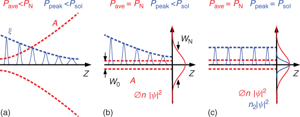
Figure 14.1 Sketch of the accessible bullet formation in NLC. (a) The pulse train disperses and diffracts in the linear regime. (b) For an average train power Pave equal to the nonlocal soliton characteristic power PN the train disperses within the soliton waveguide. The nonlocal feature is highlighted by the diffusion of the index perturbation ![]() from the illuminated region (i.e., W0
from the illuminated region (i.e., W0 ![]() WN). (c) If the pulse peak power Ppeak matches the temporal soliton characteristic power Psol, the temporal confinement occurring within the nonlocal soliton results in the formation of a train of optical bullets. The instantaneous index perturbation n2|ψ|2 matches the temporal intensity profile, and it is spatially local.
WN). (c) If the pulse peak power Ppeak matches the temporal soliton characteristic power Psol, the temporal confinement occurring within the nonlocal soliton results in the formation of a train of optical bullets. The instantaneous index perturbation n2|ψ|2 matches the temporal intensity profile, and it is spatially local.
In order to estimate the temporal properties of a pulse propagating confined in a nematicon, we formalize the wavelength dependence of the NLC indexes using a single resonance model:
14.10 ![]()
where ![]() are the strengths and
are the strengths and ![]() are the wavelengths of the resonances for
are the wavelengths of the resonances for ![]() and n||, respectively. For example, for the E7, a best-fit approach determines
and n||, respectively. For example, for the E7, a best-fit approach determines ![]() , λ|| = 182 nm, and
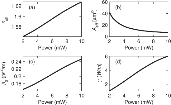
, λ|| = 182 nm, and ![]() and Γ|| = 2.083 × 10⁻⁵ [30, 32]. Then, by looking at the fundamental nonlinear modes of the system (Eqs 14.6 and 14.7), we can derive the properties of the soliton waveguides, effective index, area, GVD, and equivalent nonlinear coefficient γ as the power changes. In Figure 14.2, we considered a standard cell thickness L = 100 μm with anchoring conditions θ(X = L/2) = θ(X = − L/2) = θ0 = π/6 and NLC elastic constants K11 = K22 = K33 = 10−11N [27, 28].
and Γ|| = 2.083 × 10⁻⁵ [30, 32]. Then, by looking at the fundamental nonlinear modes of the system (Eqs 14.6 and 14.7), we can derive the properties of the soliton waveguides, effective index, area, GVD, and equivalent nonlinear coefficient γ as the power changes. In Figure 14.2, we considered a standard cell thickness L = 100 μm with anchoring conditions θ(X = L/2) = θ(X = − L/2) = θ0 = π/6 and NLC elastic constants K11 = K22 = K33 = 10−11N [27, 28].
Figure 14.2 Calculated soliton waveguides (a) effective index, (b) effective area, (c) GVD, and (d) nonlinear Kerr coefficient for an average excitation power Pave = 2.3 mW at wavelength λ = 850 nm.
It is worth noticing that for many nematics an absorption resonance is usually present in the UV range. Hence, visible and near-IR dispersion are usually normal, forbidding the formation of temporal bright soliton. However, the introduction of a small amount of a resonant dye can easily change the medium dispersion magnitude and sign around specific wavelengths.
14.3.2 Experimental Conditions for Accessible Bullets Observation
In Figure 14.3a, the effect of a diluted dye with Γres = 10−9 and resonance at λres = 930 nm on the E7 GVD can be appreciated. By assuming an excitation centered at λ = 850 nm, the dye absorption reverses the sign of the GVD and significantly affects its magnitude even for low concentrations, with negligible contributions to the medium losses in our case.
Figure 14.3 (a) β2|| and ![]() in the undoped E7 NLC (solid line) and for the case of diluted doping (Γres = 10−9) with a dye resonating at λres = 930 nm (dashed line). (b) Calculated power dependence of the soliton waveguide GVD in the presence of the dye doping at λ = 850 nm.
in the undoped E7 NLC (solid line) and for the case of diluted doping (Γres = 10−9) with a dye resonating at λres = 930 nm (dashed line). (b) Calculated power dependence of the soliton waveguide GVD in the presence of the dye doping at λ = 850 nm.
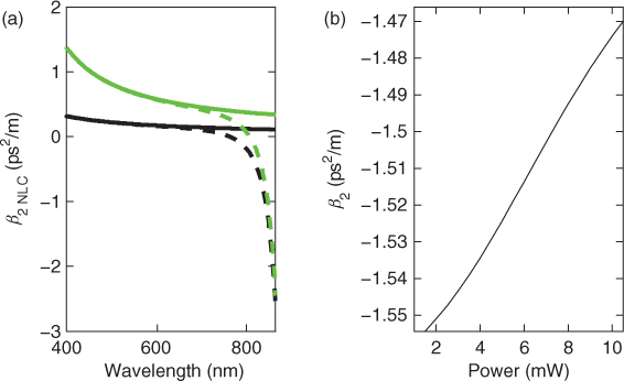
By calculating the nonlinear eigenmodes of the system (Eqs. 14.6 and 14.7), for the case of weak doping, we determine the dispersion of the soliton waveguide (Figure 14.3b) versus the soliton average power.
Figure 14.4a and 14.4b shows the temporal evolution of a T0 = 100 fs hyperbolic secant pulse ![]() centered at λ = 850 nm obtained from the Z-integration of the system (Eqs 14.6 and 14.7). The average power is Pave = 2.3 mW, which results in β2 = − 1.54 ps2/m, that is, a soliton peak power of
centered at λ = 850 nm obtained from the Z-integration of the system (Eqs 14.6 and 14.7). The average power is Pave = 2.3 mW, which results in β2 = − 1.54 ps2/m, that is, a soliton peak power of ![]() and a dispersion length of
and a dispersion length of ![]() . In particular, as expected, for Ppeak = Psol/10, the pulse disperses, whereas for Ppeak = Psol, a temporal soliton is formed. The latter case corresponds to a pulse energy of 25 pJ that imposes an excitation repetition rate of 92 MHz. As the spatial confinement is guaranteed by the average illumination properties, a train of light bullets is then formed.
. In particular, as expected, for Ppeak = Psol/10, the pulse disperses, whereas for Ppeak = Psol, a temporal soliton is formed. The latter case corresponds to a pulse energy of 25 pJ that imposes an excitation repetition rate of 92 MHz. As the spatial confinement is guaranteed by the average illumination properties, a train of light bullets is then formed.
Figure 14.4 Temporal evolution of the intensity (normalized units) of the bright pulse for T0 = 100 fs and β2 = − 1.5 ps2/m: (a) at low peak power P0 = 12.63 W, the pulse disperses in propagation, whereas (b) at high peak power P0 = 126.3 W, a bright soliton forms. The average power of the train is 2.3 mW in both cases. For comparison, the case (c) and (d) shows the evolution of a dark notch for T0 = 70 fs at the same average power 2.3 mW without resonant dye, that is, β2 = 0.166 ps2/m, with (c) P0 = 2.78 W and (d) P0 = 27.8 W.
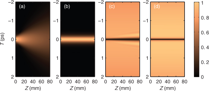
In Figure 14.4c and 14.4d, an equivalent case for a dark temporal soliton propagating confined in a spatial soliton is presented. The soliton is formed in an undoped E7-NLC and sustained by a 2.3 mW powered CW excitation, that is, β2 = 0.166ps2/m. The input field, ![]() , is a realistic excitation commonly adopted to investigate temporal dark solitons propagation. In the example, T0 = 70 fs, Tp = 5 ps (which provides a suitable pedestal), whereas the linear and nonlinear propagation examples are obtained for Ppeak = Psol/10 (Fig. 14.4c) and Ppeak = Psol (Fig. 14.4d), respectively. In this case, the train repetition rate is not a fixed parameter and depends on the chosen pedestal duration Tp. We refer to this case as antibullet [30] as it results from the combination of a bright spatial soliton solution with a dark temporal one. The examples presented earlier represent cases of stable (3 + 1)D solitary waves as they are complete solution of the general nonlinear ruling model and occurring in feasible experimental conditions. It is important to stress here that although we addressed the required balance between average power and peak power (to sustain the described regimes) in terms of source repetition rate, such balance can be reached by other means. In particular, the large difference in terms of response speed between the two involved nonlinearities in NLCs allows for a more convenient and practical approach. Once a dense pulse train is obtained from the source with the required pulse energy, a submillisecond on–off modulation (shorter than the nonlocal nonlinearity response time) is applied to the excitation: its duty cycle determines the desired average power for an arbitrary source repetition rate.
, is a realistic excitation commonly adopted to investigate temporal dark solitons propagation. In the example, T0 = 70 fs, Tp = 5 ps (which provides a suitable pedestal), whereas the linear and nonlinear propagation examples are obtained for Ppeak = Psol/10 (Fig. 14.4c) and Ppeak = Psol (Fig. 14.4d), respectively. In this case, the train repetition rate is not a fixed parameter and depends on the chosen pedestal duration Tp. We refer to this case as antibullet [30] as it results from the combination of a bright spatial soliton solution with a dark temporal one. The examples presented earlier represent cases of stable (3 + 1)D solitary waves as they are complete solution of the general nonlinear ruling model and occurring in feasible experimental conditions. It is important to stress here that although we addressed the required balance between average power and peak power (to sustain the described regimes) in terms of source repetition rate, such balance can be reached by other means. In particular, the large difference in terms of response speed between the two involved nonlinearities in NLCs allows for a more convenient and practical approach. Once a dense pulse train is obtained from the source with the required pulse energy, a submillisecond on–off modulation (shorter than the nonlocal nonlinearity response time) is applied to the excitation: its duty cycle determines the desired average power for an arbitrary source repetition rate.
14.4 Temporal Modulation Instability in Nematicons
In the demonstrated decoupled regime, we can translate all the phenomenology peculiar to the 1D nonlinear Schrödinger equation in the domain of localized temporal effect in spatial nonlocal solitons. In particular, it is possible to explore the possibility of creating dense train of optical bullets by exploiting the temporal modulational instability mechanism. At such purpose, we consider the propagation of a flat-top pulse within a nonlocal soliton waveguide (Fig. 14.5a). To stabilize the random occurrence of pulses typical of the MI phenomenon, we assume the presence of a weak CW background having wavelength slightly shifted with respect to the central flat-top wavelength.
Figure 14.5 (a) Propagation of 200 W flat top of duration τbg = 3.3 ps with a superimposed 2.3 mW background, 2.8 THz shifted in frequency. (b) Input pulse temporal profile. (c) Pulse profile after Z = 39 mm of propagation.
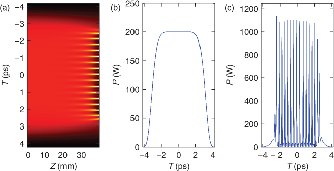
In order to get a significant amount of anomalous dispersion, we assume a dye resonance with λres = 930 nm and a pulse central wavelength λ = 850 nm (Fig. 14.3b). For an average soliton power of Pave = 2.3 mW, it turns out β2 ≈ − 1.54 ps2/m. Pave fixes the combined averaged power of pulsed pump and CW background. The CW background frequency shift depends on the peak power of the pulsed pump as the latter fixes the frequency shift of the maximum of the modulational instability gain ![]() [21]. Figure 14.5 shows the resulting propagation of a 200 W 7 ps-wide (super-Gaussian) flat top, on a 2.3 mW background (note that in this example the pump does not carry any significant average contribution) centered at wavelength λbg = 856.8 nm. In this case, a dense train of optical bullets with 2.8 THz repetition rate emerges in propagation with a maximum contrast at the Z = 39 mm. In this case, we assumed a white optical noise contribution of the same magnitude of the CW background.
[21]. Figure 14.5 shows the resulting propagation of a 200 W 7 ps-wide (super-Gaussian) flat top, on a 2.3 mW background (note that in this example the pump does not carry any significant average contribution) centered at wavelength λbg = 856.8 nm. In this case, a dense train of optical bullets with 2.8 THz repetition rate emerges in propagation with a maximum contrast at the Z = 39 mm. In this case, we assumed a white optical noise contribution of the same magnitude of the CW background.
This generation scheme requires the output section to be specifically determined (further propagation results in the mutual interaction of the formed temporal solitons). However, the position of this specific section depends on the power of the CW background; hence, it can be tuned by changing the ratio between the average power of the pulsed excitation (i.e., its repetition rate) and the CW background [32].
14.5 Soliton-Enhanced Frequency Conversion
The decoupled propagation regime described in the previous paragraphs has been recently demonstrated. In particular, third harmonic (TH) frequency conversion enhanced by a nematicon localization has been demonstrated, by exciting the third-order nonlinearity of an NLC using femtosecond pulses obtained by an optical parametric amplifier [33]. Because NLCs exhibit local inversion symmetry, considering the interaction between an FF at wavelength λFF with its TH, the source terms for the extraordinary and the ordinary component of the TH reduce, respectively, to:
14.11 ![]()
The confinement within a nonlocal soliton implies input fields preferentially e- polarized; hence, we can consider only the first source term of PTHe (eee → e type I) and the second of PTHo (eoe → o type II) relevant. The corresponding wave vector mismatches are
14.12 
14.13 
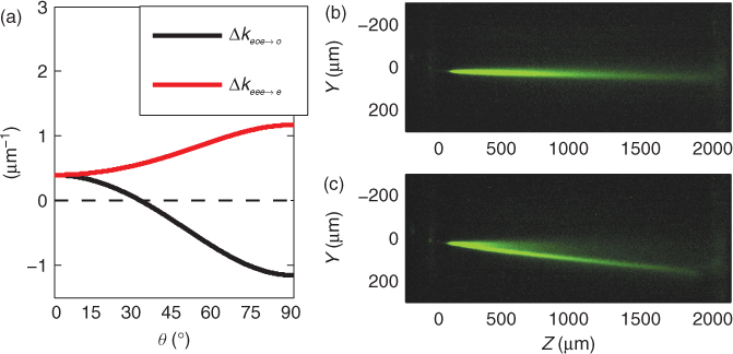
where the momenta of the extraordinary components depend on the NLC orientation. For the E7 NLC, in Figure 14.6a, the resulting phase mismatch versus the angle between o- and e- wave vectors and the director is shown.
The experimental demonstration has been performed by coupling in the NLC cell a 40 nJ, 150 fs pulsed pump beam at λ = 1500 nm of peak power Ppeak ≈ 250 kW. In the experimental Figure 14.6b, the propagation occurs at an angle of θ ≈ 31°. Type II generation is nearly in phase matching and a diffracting o-polarized THG—that is, without appreciable walk-off, emerges in propagation. Type I generation is not observed because it is not in phase matching. Conversely, if a collinear and copolarized 6 mW CW pump at λ = 1550 nm is superimposed to the pulsed excitation, a relatively strong e-TH resulting from a type I process is generated within the excited nonlocal soliton, the conversion being strongly enhanced by the tight spatial confinement. The confinement of the TH indicates its e- polarization. As the spatial profile of the TH perfectly matches the soliton waveguide, a decoupled nonlinear regime (spatial nonlocal, temporal local) is realized.
Figure 14.6 (a) Dependence of the phase mismatch Δkeee→e and Δkeoe→o from the reorientation angle θ. (b) Type II generation in bulk NLC. (c) Nematicon enhanced Type I generation.
14.6 Conclusions
In conclusion, the synergic interplay between slow-nonlocal and fast-local nonlinearities enables the access to a range of completely new experimental observable phenomena thanks to the stability arising in properly tailored illumination conditions. These results carry a large potential impact not only limited to optical systems possessing nonlinear and nonlocal optical responses (e.g., thermo-optic and photorefractive dielectrics) but also extended to physical systems where multiple nonlinear mechanisms coexist (e.g., matter waves in fluids, plasmas, and Bose–Einstein condensates).
Acknowledgments
I would like to thank Dr Alessia Pasquazi for the enlightening discussions regarding phase-matching considerations in nonlinear processes and Prof. Roberto Morandotti who made some of the measurements presented in this chapter possible. The contribution of Mr Ian Bruce Burgess to Sections 14.3 is also gratefully acknowledged. Finally, I thank Prof. Gaetano Assanto for bringing significant expertise to part of the work presented in this chapter.
1. Y. Silberberg. Collapse of optical pulses. Opt. Lett., 15(22):1282–1284, 1990.
2. E. A. Kuznetsov and V. E. Rubenchik. Soliton stability in plasmas and hydrodynamics. Phys. Rep., 142(3):103–165, 1986.
3. J. E. Bjorkholm and A. Ashkin. Cw self-focusing and self-trapping of light in sodium vapor. Phys. Rev. Lett., 32(4):129–132, 1974.
4. M. Segev, B. Crosignani, A. Yariv, and B. Fischer. Spatial solitons in photorefractive media. Phys. Rev. Lett., 68:923–926, 1992.
5. A. Dubietis, E. Gaizauskas, G. Tamosauskas, and P. Di Trapani. Light filaments without self-channeling. Phys. Rev. Lett., 92(25):253903, 2004.
6. A. Pasquazi, S. Stivala, G. Assanto, J. Gonzalo, J. Solis, and C. N. Afonso. Near-infrared spatial solitons in heavy metal oxide glasses. Opt. Lett., 32(15):2103–2105, 2007.
7. A. Pasquazi, S. Stivala, G. Assanto, J. Gonzalo, and J. Solis. Transverse nonlinear optics in heavy-metal-oxide glass. Phys. Rev. A, 77(4):043808, 2008.
8. C. Conti, M. Peccianti, and G. Assanto. Route to nonlocality and observation of accessible solitons. Phys. Rev. Lett., 91(7):073901, 2003.
9. M. Peccianti, C. Conti, G. Assanto, A. De Luca, and C. Umeton. Routing of anisotropic spatial solitons and modulational instability in liquid crystals. Nature, 432(7018):733–737, 2004.
10. Y. S. Kivshar and G. P. Agrawal. Optical Solitons: From Fibers to Photonic Crystals. Academic Press, San Diego, CA, 2003.
11. S. Trillo and W. E. Torruellas. Spatial Solitons. Springer-Verlag, Berlin, 1998.
12. A. A. Kanashov and A. M. Rubenchik. On diffraction and dispersion effect on three wave interaction. Physica D, 4(1):122–134, 1981.
13. B. A. Malomed, P. Drummond, H. He, A. Berntson, D. Anderson, and M. Lisak. Spatiotemporal solitons in multidimensional optical media with a quadratic nonlinearity. Phys. Rev. E, 56(4):4725–4735, 1997.
14. B. A. Malomed, D. Mihalache, F. Wise, and L. Torner. Spatiotemporal optical solitons. J. Opt. B: Quantum Semiclass. Opt., 7(5):R53–R72, 2005.
15. G. Fibich, B. Ilan, and G. Papanicolaou. Self-focusing with fourth-order dispersion. SIAM J. Appl. Math., 62(4):1437–1462, 2002.
16. L. C. Crasovan, J. P. Torres, D. Mihalache, and L. Torner. Arresting wave collapse by wave self-rectification. Phys. Rev. Lett., 91(6):63904, 2003.
17. H. Leblond. Bidimensional optical solitons in a quadratic medium. J. Phys. A: Math. Gen., 31:5129–5143, 1998.
18. H. Leblond. Propagation of optical localized pulses in chi2 crystals: A (3 + 1)-dimensional model and its reduction to the NLS equation. J. Phys. A: Math. Gen., 31:3041–3066, 1998.
19. J. P. Torres, S. L. Palacios, L. Torner, L.-C. Crasovan, D. Mihalache, and I. Biaggio. Method for generating solitons sustained by competing nonlinearities by use of optical rectification. Opt. Lett., 27(18):1631–3, 2002.
20. J. P. Torres, L. Torner, I. Biaggio, and M. Segev. Tunable self-action of light in optical rectification. Opt. Commun., 213(4–6):351–356, 2002.
21. G. P. Agrawal. Nonlinear Fiber Optics, 3rd edn. Academic Press, New York, 2001.
22. D. Mihalache, D. Mazilu, F. Lederer, B. A. Malomed, Y. Kartashov, L. C. Crasovan, and L. Torner. Three-dimensional spatiotemporal optical solitons in nonlocal nonlinear media. Phys. Rev. E, 73(2):4–7, 2006.
23. F. W. Dabby and J. R. Whinnery. Thermal self-focusing of laser beams in lead glasses. Appl. Phys. Lett., 13(8):284–286, 1968.
24. C. Rotschild, B. Alfassi, O. Cohen, and M. Segev. Long-range interactions between optical solitons. Nat. Phys., 2(11):769–774, 2006.
25. G. Duree, J. Shultz, G. Salamo, M. Segev, A. Yariv, B. Crosignani, P. Di Porto, E. Sharp, and R. Neurgaonkar. Observation of self-trapping of an optical beam due to the photorefractive effect. Phys. Rev. Lett., 71(4):533–536, 1993.
26. M. Mitchell, Z. G. Chen, M. F. Shih, and M. Segev. Self-trapping of partially spatially incoherent light. Phys. Rev. Lett., 77(3):490–493, 1996.
27. P. G. de Gennes and J. Prost. The Physics of Liquid Crystals, 2nd edn. Oxford University Press, London, 1995.
28. I. C. Khoo. Nonlinear optics of liquid crystalline materials. Phys. Rep., 471(5–6):221–267, 2009.
29. M. Peccianti and G. Assanto. Nematic liquid crystals: A suitable medium for self-confinement of coherent and incoherent light. Phys. Rev. E, 65(3):35603, 2002.
30. I. B. Burgess, M. Peccianti, G. Assanto, and R. Morandotti. Accessible light bullets via synergetic nonlinearities. Phys. Rev. Lett., 102(20):203903, 2009.
31. M. Peccianti, C. Conti, and G. Assanto. Optical modulational instability in a nonlocal medium. Phys. Rev. E, 68:25602, 2003.
32. M. Peccianti, I. B. Burgess, G. Assanto, and R. Morandotti. Space-time bullet trains via modulation instability and nonlocal solitons. Opt. Express, 18(6):5934–41, 2010.
33. M. Peccianti, A. Pasquazi, G. Assanto, and R. Morandotti. Enhancement of third-harmonic generation in nonlocal spatial solitons. Opt. Lett., 35:3342–4, 2010.