
14
A Zoning System and Some Examples
14.1 General Introduction
The program fem_2d_1.m presented in Chapter 13 is a general two-dimensional (2d) FEM program. It can handle sophisticated geometries. On the other hand, starting with a structure description and creating the zoning (also called the meshing or the tessellation), which generates the input files for this program, is a complex problem in its own right. Although generating an unstructured grid for a complex geometry by hand is not literally impossible, it is so difficult and the results would probably be so erroneous, that it would be a pointless quest. Computer-aided mesh generation is necessary.
Fortunately, for both academic and commercial purposes, many software packages have been developed. Some relatively simple packages were presented in the MoM unstructured grid discussed earlier. As was also discussed earlier, an in depth analysis or development of one of these programs is outside the scope of this book. On the other hand, we can't proceed with FEM examples or study the electrostatic properties of structures that FEM modeling would enable without a meshing system.
In this chapter we'll introduce the gmsh package; gmsh is a free three-dimensional (3d) FEM grid generator that may be downloaded along with very extensive documentation and tutorials (hhtp://geuz.org/gmsh/).1 It is distributed under the GNU General Public License.2 In the introduction to gmsh that follows, only a very small subset of gmsh capabilities is presented. The program(s) shown that read gmsh output files and parse the data for use by our MATLAB FEM programs were written only to handle the uses of gmsh discussed here. In other words, if you choose to extend your understanding and use of gmsh beyond what is presented, be prepared to extend the gmsh file parsing programs and possibly the FEM analysis programs to include these previously unconsidered capabilities.
14.2 Introduction to gmsh
The gmsh program is available in Windows, Macintosh, or Linux formats at http://geuz.org/gmsh/. The gmsh installation includes a full documentation manual. This manual, in turn, includes a full tutorial. There are also many other tutorials and examples available online.
A gmsh structure description may be constructed and modified interactively, by directly editing a data file, or by a combination of both of these techniques. The procedures for these approaches are described in the gmsh tutorials. In this chapter only data file input will be considered. This is not limiting in any way — all lines entered into a file using a text editor become part of the structure, and all information added interactively to the structure become lines in the file.
Starting gmsh, moving and sizing the windows as necessary and bringing up a drawing description file (xx.geo) in a text editor should be learned from the documentation/and/or tutorials. Any American Standard Code for Information Interchange (ASCII) text editor will work for editing gmsh files. An editor that displays line numbers is preferable for these discussions because referring to line numbers is an excellent and easy way to discuss the file's contents. The struct14_1.geo file — a simple gmsh rectangular plane description — is as follows:
// Gmsh structure file struct14_1.geo
lc = 1.;
// create a rectangular surface loop
Point(1) = {-2, -1, 0, lc};
Point(2) = {2, -1, 0, lc};
Point(3) = {2, 1, 0, lc};
Point(4) = {-2, 1, 0, lc};
Line(1) = {1, 2};
Line(2) = {2, 3};
Line(3) = {3, 4};
Line(4) = {4, 1};
Line Loop(3) = {1, 2, 3, 4};
Plane Surface(4) = {3} ;
The file struct14_1.geo displays the basic syntax of gmsh operation. Line 1 is a comment line. The // in a line denotes that everything following on that line is a comment; as in most programming languages, comments are ignored by the program.
Lines 2 (and lines 4, 6, etc.) are blank lines that are ignored by the program. Their purpose is to make groupings of content lines easier for a reader's eye to follow.
Line 3 defines the variable lc and sets it equal to one. (lc means characteristic length and will be discussed further below). The actual name of the variable is arbitrary.
Lines 7–10 each define a point. Each point has a unique number (1–4 in this example). The choice of numbers is arbitrary insofar as gmsh is concerned. Certain numbering conventions will be defined below to pass information to the MATLAB functions. (This is not part of gmsh or MATLAB, but rather “invented” conventions for our programs.) Each point has three coordinates and a characteristic length. In this example all four lines have the same characteristic length. This is not a necessary restriction — other variables could have been defined, and/or values have been entered directly into each point's description.
Lines 12–15 each define a line connecting two points. Again, line numbers are unique arbitrary choices. Note that the line numbers are independent of the point numbers. The order of the points in each line definition is arbitrary, but will be relevant when lines are connected.
Line 17 defines a line loop, namely, a polygon, in this case a closed rectangle. If the numbering of the line segments is taken as {tail, head}, then the head of one segment should connect to the tail of the next in the loop. If line 2 is defined as {3, 2} instead of {2, 3}, then line 17 would have to be modified to {1, -2, 3, 4} to preserve the definition of the simple rectangle.
Line 18 defines a plane surface as the area enclosed by line loop 3.
Figure 14.1 shows the structure described by struct14_1.geo. This is the structure that should be visible in the gmsh display window. When the gmsh display window is the active window, hovering the cursor over one of the corners of the rectangle (a defined point) will cause the point number and its vertices to be listed at the bottom of the window. Similarly, hovering the cursor over one of the lines will produce a listing of the line number and its defining points. The dashed lines inside the rectangle reflect the fact that this is a defined plane, and hovering the cursor over a dashed line will produce the plane number and its defining lines.
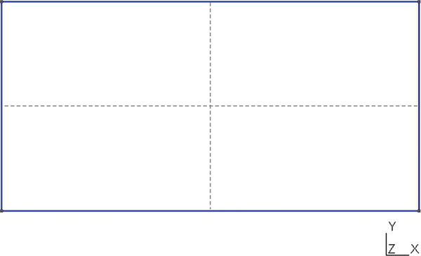
FIGURE 14.1 The gmsh structure described by struct14_1.geo.
If the upper choice box in the gmsh control window is switched to mesh (it should have been at its opening choice of geometry) and the 2D choice is selected, the rectangle is meshed into triangles (Figure 14.2).
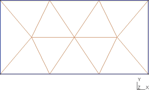
FIGURE 14.2 struct14_1.geo showing 2d meshing (lc = 1).
Since the boundaries of a rectangle are straight lines, no compromises had to be made – the surface is entirely filled with triangles. If we want higher-resolution meshing, all we have to do is reduce the value of lc and repeat the meshing operation.
Figure 14.3 shows the meshing for lc reduced to 0.25.
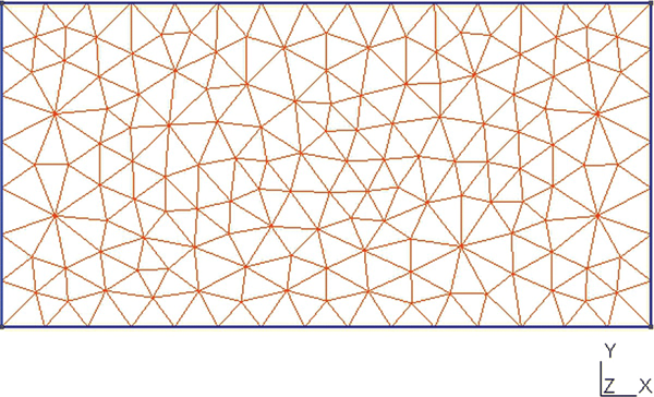
FIGURE 14.3 struct14_1.geo showing finer meshing (lc = 0.25).
The use of one or more characteristic lengths is now apparent. This number determines how finely gmsh will subdivide a surface into a mesh. Also, note that now there is no regularity to the location of the nodes. This is an unstructured meshing; there is no simple formula that can calculate a node number from the node's location, or vice versa.
Here is gmsh file struct14_2.geo — a gmsh transmission line cross sectional structure:
// Gmsh structure struct14_2.geo
lc = .5;
// exterior loop
Point(1) = {-2, -1, 0, lc};
Point(2) = {2, -1, 0, lc};
Point(3) = {2, 1, 0, lc};
Point(4) = {-2, 1, 0, lc};
Line(1) = {1, 2};
Line(2) = {2, 3};
Line(3) = {3, 4};
Line(4) = {4, 1};
// interior surface which will become a hole
Point(5) = {-1, -.05, 0, lc};
Point(6) = {1, -.05, 0, lc};
Point(7) = {1, .05, 0, lc};
Point(8) = {-1, .05, 0, lc};
Line(105) = {5, 6};
Line(106) = {6, 7};
Line(107) = {7, 8};
Line(108) = {8, 5};
Line Loop(1) = {105, 106, 107, 108};
Plane Surface(200) = {1};
// exterior surface
Line Loop(3) = {1, 2, 3, 4};
Plane Surface(4) = {3, 1} ;
Program struct14_2.geo begins as a repeat of struct14_1.geo, up through line 13. The line loop and plane surface commands of struct14_1.geo, however, have been removed.
Then struct14_2.geo defines four new points (lines 16–19), and then four new lines (lines 21–24), which form a small rectangle, inside the first rectangle. Lines 26 and 27 then create a line loop and define a plane surface.
Line 30 defines line loop 3 for the first rectangle. It could have been left where it was originally, but was moved to keep it with it corresponding plane surface command, line 31. This plane surface command has two arguments: {3, 1}. The first number, 3, refers to line loop 3. This is the outer rectangle's surface area. The second number, 1 (and any other numbers, if they are present), refers to line loops that are internal to line loop 3, and are “holes” in that surface.
Figure 14.4 shows the structure that has been defined. It is the structure of the cross section of a rectangular transmission line with a rectangular center conductor.

FIGURE 14.4 Structure defined by struct14_2.geo.
The lines of the inner rectangle are numbered by integers between 100 and 199. The plane surface defined by this line loop is numbered by an integer between 200 and 299. These choices are not gmsh-based. They are chosen, as will be seen in Section 14.3, to facilitate using this structural definition as an electrostatics description — that is, as an easy way to tell upcoming software how to identify an inner conductor (inside the outer boundary).
Figure 14.5 shows the result of the 2d meshing of struct14_2.geo.

FIGURE 14.5 Two-dimensional meshing of struct14_2.geo.
This figure shows that gmsh is smart enough to understand that the characteristic length chosen for all the line segments is too great for the short sides of the inner rectangle. It adjusts triangle sizes automatically and produces a mesh that is very usable for electrostatic modeling. The overall characteristic length could, of course, always be reduced and/or individual regions tweaked as desired.
The last thing we need to do with this structure in gmsh is to choose Save in the mesh dropdown list gmsh will create the file struct14_2.msh.
14.3 Translating the gmsh.msh File
The file struct14_2.msh is an ASCII text file. While computers will have no trouble reading it, it is a difficult file to read by eye; floating-point numbers are 15 digits long and a single space separates columns. The file struct14_2_edited.msh.txt is, as its name implies, an edited version of struct14_2.msh; the floating-point numbers are rounded to three digits and the columns have tab separators. Here is struct14_2_ edited.msh.txt— the struct14_2.msh file reformatted for easier reading:
$ MeshFormat
2.2  0  8
$EndMeshFormat
$Nodes
99
1   -2      -1        0
2    2       -1        0
3    2        1        0
4   -2        1        0
5   -1      -0.05      0
6    1       -0.05      0
7    1        0.05     0
8   -1        0.05     0
9   -1.429         -1       0
10   -0.857    -1      0
11   -0.286    -1      0
12   0.286    -1      0
13   0.857    -1      0
14   1.429    -1      0
15   2       -0.333    0
16   2      0.333          0
17   1.429    1       0
18   0.857     1        0
19   0.286     1      0
20   -0.286     1       0
21   -0.857    1        0
22   -1.429           1       0
23   -2        0.333     0
24   -2      -0.333     0
25   -0.333          -0.05      0
26    0.333    -0.05      0
27   0.333    0.05     0
28   -0.333    0.05       0
29    -1.599          0       0
30    1.599    0        0
31    1.316    0.474      0
32   -1.316    -0.474       0
33   -1.316   0.474    0
34    1.316  -0.474    0
35   -0.84   -0.547     0
36    0.84     0.547     0
37     0.84   -0.547     0
38   -0.84     0.547     0
39    1.269   0        0
40   -1.269   0       0
41   -1.185          -0.256    0
42    1.185          0.256    0
43    -1.185     0.256    0
44     1.185    -0.256    0
45     0.94    -0.27     0
46    -0.94       0.27     0
47    -0.94      -0.27     0
48     0.94     0.27     0
49     0       -0.536    0
50     0          0.536    0
51     1.109      0        0
52    -1.109      0         0
53    -1.609    -0.643     0
54     1.609    0.643      0
55     1.609     -0.643       0
56    -1.609    0.643       0
57    -0.462    0.576       0
58     0.462    -0.576       0
59    -0.462    -0.576      0
60     0.462    0.576    0
61    -1.469             -0.255     0
62     1.469    0.255    0
63    -1.469    0.255    0
64     1.469     -0.255          0
65     1.103      0.121      0
66    -1.103    -0.121     0
67    -1.103     0.121       0
68     1.103    -0.121       0
69    -1.09    -0.464       0
70     1.09     0.464    0
71     -1.09     0.464    0
72     1.09    -0.464    0
73     0.646    -0.295    0
74     0.746    -0.15       0
75    -0.646     0.295       0
76    -0.746    0.15       0
77     0.646    0.295       0
78     0.746    0.15       0
79    -0.646              -0.295   0
80    -0.746    -0.15      0
81    -1.187             -0.718    0
82     1.187    0.718     0
83    -1.187    0.718     0
84     1.187    -0.718     0
85     0.667    0          0
86    -0.667    0       0
87     0       0       0
88    -0.211    0       0
89     0.455    0       0
90    -0.455    0        0
91     0.878    0        0
92    -0.878    0        0
93     0.211    0        0
94    -0.282    0       0
95    -0.385    0        0
96      0.385    0        0
97      0.948    0        0
98    -0.948    0        0
99      0.282    0        0
$EndNodes
$Elements
212
1   15  2  0  1   1
2   15  2  0  2   2
3   15  2  0  3   3
4   15  2  0  4   4
5   15  2  0  5   5
6   15  2  0  6   6
7   15  2  0  7   7
8   15  2  0  8   8
9   1  2  0  1    1   9
10  1  2  0  1    9   10
11  1  2  0  1    10  11
12  1  2  0  1    11  12
13  1  2  0  1    12  13
14  1  2  0  1    13  14
15  1  2  0  1    14  2
16  1  2  0  2    2   15
17  1  2  0  2    15  16
18  1  2  0  2    16  3
19  1  2  0  3   3    17
20  1  2  0  3    17  18
21  1  2  0  3    18  19
22  1  2  0  3    19  20
23  1  2  0  3    20  21
24  1  2  0  3    21  22
25  1  2  0  3    22  4
26  1  2  0  4   4   23
27  1  2  0  4    23  24
28  1  2  0  4     24  1
29  1  2  0  105  5   25
30  1  2  0  105  25  26
31  1  2  0  105  26  6
32  1  2  0  106  6   7
33  1  2  0  107  7   27
34  1  2  0  107  27  28
35  1  2  0  107  28  8
36  1  2  0  108  8   5
37  2  2  0  4     7   65  48
38  2  2  0  4     5   66  47
39  2  2  0  4     8   46  67
40  2  2  0  4     6   45  68
41  2  2  0  4    31  62  54
42  2  2  0  4    32  61  53
43  2  2  0  4    33  56  63
44  2  2  0  4    34  55  64
45  2  2  0  4  15  30  64
46  2  2  0  4  23  29  63
47  2  2  0  4  16  62  30
48  2  2  0  4  24  61  29
49  2  2  0  4 6  51  7
50  2  2  0  4 5 8    52
51  2  2  0  4  15  64  55
52  2  2  0  4  23  63  56
53  2  2  0  4  16  54  62
54  2  2  0  4  24  53  61
55  2  2  0  4 8  76  46
56  2  2  0  4 6  74  45
57  2  2  0  4 7  48  78
58  2  2  0  4 5  47  80
59  2  2  0  4  13  37  58
60  2  2  0  4  21  38  57
61  2  2  0  4  18  60  36
62  2  2  0  4  10  59  35
63  2  2  0  4  23  24  29
64  2  2  0  4  15  16  30
65  2  2  0  4  32  53  81
66  2  2  0  4  31  54  82
67  2  2  0  4  33  83  56
68  2  2  0  4  34  84  55
69  2  2  0  4  39  42  65
70  2  2  0  4  40  41  66
71  2  2  0  4  40  67  43
72  2  2  0  4   39  68  44
73  2  2  0  4 1  53  24
74  2  2  0  4 3  54  16
75  2  2  0  4 4  23  56
76  2  2  0  4 2  15  55
77  2  2  0  4  12  13  58
78  2  2  0  4  20  21  57
79  2  2  0  4  18  19  60
80  2  2  0  4  10  11  59
81  2  2  0  4  11  12  49
82  2  2  0  4  19  20  50
83  2  2  0  4  17  18  82
84  2  2  0  4 9  10  81
85  2  2  0  4  21  22  83
86  2  2  0  4  13  14  84
87  2  2  0  4  25  49  26
88  2  2  0  4  27  50  28
89  2  2  0  4  41  47  66
90  2  2  0  4  42  48  65
91  2  2  0  4  43  67  46
92  2  2  0  4  44  68  45
93  2  2  0  4  39  65  51
94  2  2  0  4  40  66  52
95  2  2  0  4  40  52  67
96  2  2  0  4  39  51  68
97   2  2  0  4  13  84  37
98   2  2  0  4  21  83  38
99   2  2  0  4  10  35  81
100  2  2  0  4  18  36  82
101  2  2  0  4  1   9    53
102  2  2  0  4  3   17  54
103  2  2  0  4  2   55  14
104  2  2  0  4  4   56  22
105  2  2  0  4  36  70  82
106  2  2  0  4  35  69  81
107  2  2  0  4  37  84  72
108  2  2  0  4  38  83  71
109  2  2  0  4  5   52  66
110  2  2  0  4  7   51  65
111  2  2  0  4  8   67  52
112  2  2  0  4  6   68  51
113  2  2  0  4  9   81  53
114  2  2  0  4  17  82  54
115  2  2  0  4  22  56  83
116  2  2  0  4  14  55  84
117  2  2  0  4  26  49  58
118  2  2  0  4  28  50  57
119  2  2  0  4  25  59  49
120  2  2  0  4  27  60  50
121  2  2  0  4  12  58  49
122  2  2  0  4  20  57  50
123  2  2  0  4  19  50  60
124  2  2  0  4  11  49  59
125  2  2  0  4  40  61  41
126  2  2  0  4  39  62  42
127  2  2  0  4  40  43  63
128  2  2  0  4  39  44  64
129  2  2  0  4  27  77  60
130  2  2  0  4  25  79  59
131  2  2  0  4  26  58  73
132  2  2  0  4  28  57  75
133  2  2  0  4  32  41  61
134  2  2  0  4  31  42  62
135  2  2  0  4  33  63  43
136  2  2  0  4  34  64  44
137  2  2  0  4  45  74  73
138  2  2  0  4  46  76  75
139  2  2  0  4  48  77  78
140  2  2  0  4  47  79  80
141  2  2  0  4  26  73  74
142  2  2  0  4  28  75  76
143  2  2  0  4  27  78  77
144  2  2  0  4  25  80  79
145  2  2  0  4  41  69  47
146  2  2  0  4  42  70  48
147  2  2  0  4  43  46  71
148  2  2  0  4  44  45  72
149  2  2  0  4    37  73  58
150  2  2  0  4    38  75  57
151  2  2  0  4    36  60  77
152  2  2  0  4    35  59  79
153  2  2  0  4    37  45  73
154  2  2  0  4    38  46  75
155  2  2  0  4    36  77  48
156  2  2  0  4    35  79  47
157  2  2  0  4    29  61  40
158  2  2  0  4    30  62  39
159  2  2  0  4    30  39  64
160  2  2  0  4    29  40  63
161  2  2  0  4    32  81  69
162  2  2  0  4    31  82  70
163  2  2  0  4    33  71  83
164  2  2  0  4    34  72  84
165  2  2  0  4    32  69  41
166  2  2  0  4    31  70  42
167  2  2  0  4    34  44  72
168  2  2  0  4    33  43  71
169  2  2  0  4    38  71  46
170  2  2  0  4    37  72  45
171  2  2  0  4    36  48  70
172  2  2  0  4    35  47  69
173  2  2  0  4    26  74  6
174  2  2  0  4    27  7   78
175  2  2  0  4    28  76  8
176  2  2  0  4   5    80  25
177  2  2  0  200  25  94  28
178  2  2  0  200  26  96  27
179  2  2  0  200  25  28  95
180  2  2  0  200  5   98  8
181  2  2  0  200  6   7   97
182  2  2  0  200  26  27  99
183  2  2  0  200  91  97  7
184  2  2  0  200  27  93  99
185  2  2  0  200  92  8   98
186  2  2  0  200  5   92  98
187  2  2  0  200  85  91  7
188  2  2  0  200  28  94  88
189  2  2  0  200  28  90  95
190  2  2  0  200  26  99  93
191  2  2  0  200  86  8   92
192  2  2  0  200  27  96  89
193  2  2  0  200  27  87  93
194  2  2  0  200  26  6    85
195  2  2  0  200  26  89  96
196  2  2  0  200  25  90  86
197  2  2  0  200  27  89  85
198  2  2  0  200  27  85  7
199  2  2  0  200  5   86  92
200  2  2  0  200  28  86  90
201  2  2  0  200  85  6   91
202  2  2  0  200  26  85  89
203  2  2  0  200  25  87  88
204  2  2  0  200  25  95  90
205  2  2  0  200  25  88  94
206  2  2  0  200  25  26  87
207  2  2  0  200  28  88  87
208  2  2  0  200  91  6   97
209  2  2  0  200  27  28  87
210  2  2  0  200  26  93  87
211  2  2  0  200  28  8   86
212  2  2  0  200  5   25  86
$EndElements
The program parse_msh_file.m translates the gmsh mesh file struct14_2.msh to the three data files that fem_2d_1.m requires as discussed in the last chapter. File parse_msh_file.m is not a general-purpose gmsh–to–MATLAB conversion program. It handles only those gmsh capabilities discussed in these chapters. It performs limited validity checking, and, while it prompts for an output file name, it does not check to see whether that name is already in use.
If parse_msh_file.m succeeds, it returns the three files nodes_filename.txt, trs_filename.txt, and bcs_filename.txt, where filename is a user-supplied name. If the program fails for any reason, the three output files are generated, but they are empty files.
File parse_msh_file.m parses struct14_2.msh using the following algorithms:
- Lines 10 and 11. Get the name of the
.mshfile to read; open the file (for reading). - Lines 13–31. Verify the header information.
- Lines 33–59. Read node location information and store in nodes array.
- Lines 60–91. Read triangle and boundary condition information and store in
trsandbcsarrays. The Column 2 in the.mshfile in this section indicates an element type: 15 = point, 1 = line, 2 = 3 node triangle. Points entries are ignored. Triangle entries, except for excluded regions, are added to thetrsarray. Line entries are added to thebcsarray. - Line 92. Close the input file
- Lines 94–103. List the bcs file, prompt for lines to become 1-V boundary conditions (the default is 0 V).
- Lines 105–117. Prompt for the output file name and write the files to disk.
Program parse_msh_file.m — MATLAB script for converting gmsh output for FEM analysis usage — is as follows:
% parse_msh_file.m
% Read the mesh file generated by gmsh and parse it
% This is a very limited routine, based only on the
%   capabilities of gmsh that are being used
% Element types handled are 1 = line, 2 = 3 node triangle, 15 = point
 clear
 filename = uigetfile('*.msh'), % read the file
 fid = fopen(filename, 'r'),
 tline = fgetl(fid); % read the first file line
 if (strcmp(tline, '$MeshFormat')) == 0 % Verify file type
  'Problem with this file'
  nodes = []; trs = []; bcs = [];
  fclose (fid);
  return
 end
 tline = fgetl(fid); % look for version number
 [header] = sscanf(tline, '%f %d %d'),
 if (header(1) ~ = 2.2), 'Possible gmsh version incompatibility', end;
 tline = fgetl(fid); % Look for $EndMeshFormat
 if (strcmp(tline, '$EndMeshFormat')) == 0
  'No $EndMeshFormat Line found'
  nodes = []; trs = []; bcs = [];
  fclose (fid);
  return
 end
 tline = fgetl(fid); % Look for $Nodes
 if (strcmp(tline, '$Nodes')) == 0
  'No $Nodes Line found'
  nodes = []; trs = []; bcs = [];
  fclose (fid);
  return
 end
% NOTE: Nodes is being read as a 3-d file even though only 2-d
%   usage is anticipated in this version
nr_nodes = fscanf(fid, '%d', 1); % get number of nodes
nodes = [0,0,0]; % zeros(nr_nodes, 3); % allocate nodes array
for i = 1 : nr_nodes % get nodes information
 temp = fscanf(fid, '%g', 4);
 n = temp(1);
 nodes(n,:) = temp(2:4);
end
fgetl(fid);   % Clear the line
tline = fgetl(fid);   % Look for $EndNodes
if (strcmp(tline, '$EndNodes')) == 0
 'No $EndNodes Line found'
 nodes = []; trs = []; bcs = [];
 fclose (fid);
 return
end
tline = fgetl(fid); % Look for $Elements
if (strcmp(tline, '$Elements')) == 0
 'No $Nodes Line found'
 nodes = []; trs = []; bcs = [];
 fclose (fid);
 return
end
trs = []; bcs = [];
nr_elements = fscanf(fid, '%d', 1); % get number of elements
for i = 1: nr_elements        % process elements information
 temp = fscanf(fid, '%d %d', 2);   % get element type
 if temp(2) == 15          % defined point
  fgetl(fid);            % clear the line
 elseif temp(2) == 1        % defined line
  temp2 = fscanf(fid, '%d %d %d %d %d', 5);
  bcs = [bcs; [temp2(3:4)', 0]];
  fgetl(fid);
 elseif temp(2) == 2        % created mesh triangle
  temp3 = fscanf(fid, '%d %d %d %d %d %d', 6);
  if temp3(3) < 200         % ignore excluded triangles
   trs = [trs; temp3(4:6)'];
  end
  fgetl(fid);
 else
  'Unknown type in mesh file'
  nodes = []; trs = []; bcs = [];
  fclose (fid);
  return
 end
end
fclose (fid);
nr_bc_lines = length(bcs);
while 1 == 1
 'bcs file: '
 bcs
 line_fix = input('Enter line # to set 1 volt bc, 0 to conclude: '),
 if line_fix == 0, break, end;
 for i = 1 : nr_bc_lines
  if bcs(i,1) == line_fix, bcs(i,3) = 1; end;
 end
end
filename = input('Name for output files, NO OVERWRITE CHECKING: ', 's'),
nodes_file_name = strcat('nodes_', filename, '.txt'),
trs_file_name = strcat('trs_', filename, '.txt'),
bcs_file_name = strcat('bcs_', filename, '.txt'),
fid = fopen (nodes_file_name, 'w'),
fprintf (fid, '%g	%g	%g
', nodes'),
fclose (fid);
fid = fopen (trs_file_name, 'w'),
fprintf (fid, '%d	%d	%d
', trs'),
fclose (fid);
fid = fopen (bcs_file_name, 'w'),
fprintf (fid, '%d	%d	%d
', bcs'),
fclose (fid);
Item 6 in the list preceding this program deserves some discussion. The program first presents the boundary condition file as listed in the following table; only the last 12 lines of the file are shown in this table:
| Line Number | Node Number | Boundary Condition |
| 3 | 22 | 0 |
| 4 | 4 | 0 |
| 4 | 23 | 0 |
| 4 | 24 | 0 |
| 105 | 5 | 0 |
| 105 | 25 | 0 |
| 105 | 26 | 0 |
| 106 | 6 | 0 |
| 107 | 7 | 0 |
| 107 | 27 | 0 |
| 107 | 28 | 0 |
| 108 | 8 | 0 |
The first column in the table (i.e., in the file) is the line number from the original.geo file. Since the data being processed are of the fully meshed structure, there is typically more than one line section (triangle side) associated with each of these line numbers. The second column contains one of the nodes associated with the line segment. If we restrict ourselves to conductors having a closed surface and nonzero enclosed area, then only one node number is necessary. The last column shows the boundary condition associated with this node. The original, default, value as shown for all nodes is 0 V.
The program prompt at this point reads Enter line # to set 1 volt bc, 0 to conclude: The response to this prompt could be any of the line numbers shown in the table. The reason for numbering internal electrodes with line numbers > 100 is now apparent; these line segments appear at the end of the list and are easy to identify.
A response of 105 (with a carriage return) causes the file to be modified and reprinted as follows:
| Line Number | Node Number | Boundary Condition |
| 3 | 22 | 0 |
| 4 | 4 | 0 |
| 4 | 23 | 0 |
| 4 | 24 | 0 |
| 105 | 5 | 1 |
| 105 | 25 | 1 |
| 105 | 26 | 1 |
| 106 | 6 | 0 |
| 107 | 7 | 0 |
| 107 | 27 | 0 |
| 107 | 28 | 0 |
| 108 | 8 | 0 |
As this table shows, all nodes associated with the original line 105 have been set to 1 V. Repeating this procedure, entering 106, 107, and 108 (in any order) produces the desired file, as listed in the following table:
| Line Number | Node Number | Boundary Condition |
| 3 | 22 | 0 |
| 4 | 4 | 0 |
| 4 | 23 | 0 |
| 4 | 24 | 0 |
| 105 | 5 | 1 |
| 105 | 25 | 1 |
| 105 | 26 | 1 |
| 106 | 6 | 1 |
| 107 | 7 | 1 |
| 107 | 27 | 1 |
| 107 | 28 | 1 |
| 108 | 8 | 1 |
The entire inner conductor surface has now been set to 1 V and the file is ready for use. A response of 0 terminates this part of the program; the program then moves on to writing the newly generated data files to disk.
14.4 Running the FEM Analysis
The data files are now ready for fem_2d_1.m (described and listed in Chapter 13). The program produces Figures 14.6 and 14.7.
FIGURE 14.6 gmsh zoning of struct14_2.geo showing boundary conditions.
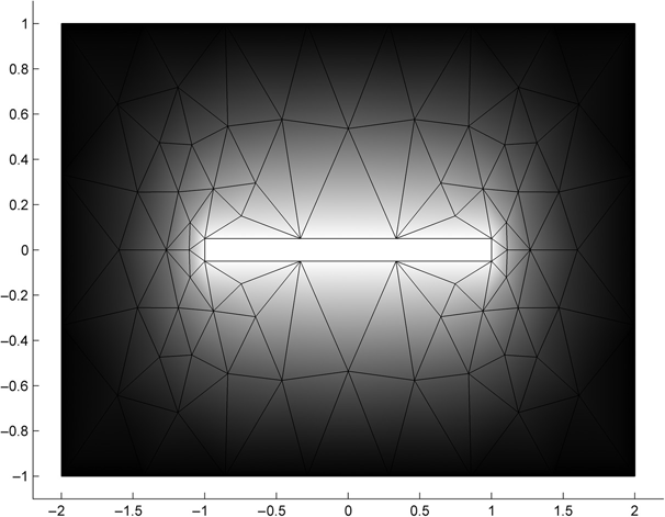
FIGURE 14.7 Graphical output of fem_2d_1 showing voltage profile.
Repeating a note from Chapter 13, removing the line near the bottom of the show_mesh.m function colormap (gray) will produce an on-screen version of Figure 14.7 with color interpretation of the voltage distribution.
Program fem_2d_1.m also calculates the capacitance of the structure, C = 58.97 pF/m. An online calculator of stripline impedance3 predicts C = 55.6 pF/m. Even with the sides of the box as close as they are to the center conductor, the FEM prediction is high.
Increasing the outer box sidewall positions to 3 m and decreasing the characteristic length (lc) to 0.1 reduces the capacitance error to < 0.5%.
14.5 More gmsh Features and Examining the Electric Field
File struct14_3.geo illustrates several additional gmsh features, all of which require no modification of parse_msh_file.m or fem_2d_1.m for use:
// gmsh structure file struct14_3.geo
lc = .1;
// exterior loop
Point(1) = {-1.5, -1.5, 0, lc};
Point(2) = {1.5, -1.5, 0, lc};
Point(3) = {1.5, 1.5, 0, lc};
Point(4) = {-1.5, 1.5, 0, lc};
Line(1) = {1, 2};
Line(2) = {2, 3};
Line(3) = {3, 4};
Line(4) = {4, 1};
// interior surface which will become a hole
Point(5) = {-.5, -.5, 0, lc};
Point(6) = {.5, -.5, 0, lc};
Point(7) = {.5, 0, 0, lc};
Point(8) = {-.5, 0, 0, lc};
Point(9) = {0, 0, 0, lc};
Line(105) = {8, 5};
Line(106) = {5, 6};
Line(107) = {6, 7};
Circle(108) = {7, 9, 8};
// rotate the inner conductor about the z axis
a = 3.1416/4;
Rotate {{0,0,1},{0,0,0},a}{Point{5};Point{6};Point{7};Point{8};Point{9};}
Line Loop(1) = {105, 106, 107, 108};
Plane Surface(200) = {1};
// exterior surface
Line Loop(3) = {1, 2, 3, 4};
Plane Surface(4) = {3, 1} ;
The structure produced by struct14_3.geo (with the boundary conditions tabulated and the meshing shown) is shown in Figure 14.8.
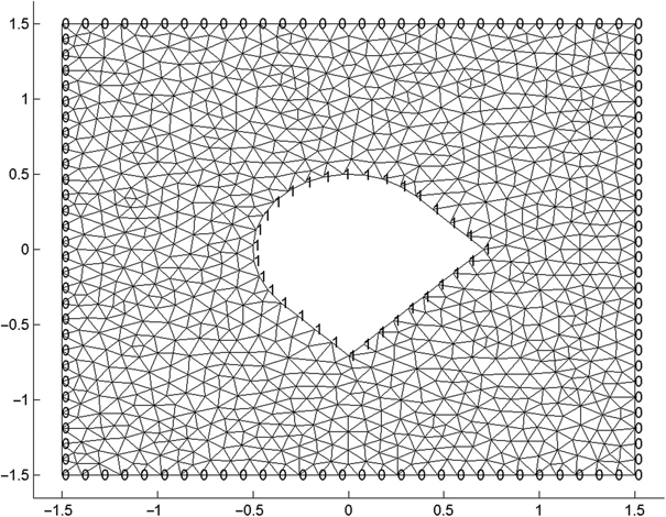
FIGURE 14.8 Structure produced by struct14_3.geo.
Referring to the struct14_3.geo listing, points 1–4 and lines 1–4 define an outer box. Points 5–8 define a rectangle, but lines 105–108 only connect three sides of this rectangle. Point 9 defines a fifth point that lies midway between points 7 and 8. Circle 108 defines the arc of a circle connecting points 7 and 9, with its center at point 8. The rotate instruction rotates points 5–9 about the Z axis by 45o (π/4 radians). This is an arbitrary rotation used only to show the capability.
There is also a command for translating a group of points. At first glance this seems unnecessary — why not just define the points at their final locations? Translation, however, is very valuable for facilitating parameter studies, such as moving the inner conductor about and studying the results on the structure's fields, capacitance, and other properties. Translation, together with an available duplication command, allows for placement of multiple complex electrode shapes in a structure at arbitrary locations. Combining all of these capabilities (translation, duplication, and rotation) allows for easy generation and manipulation of complex structures.
Returning to Figure 14.8, the boundary conditions are 0 V on the outer (square) boundary and 1 V on the inner conductor. The former boundary condition is set by default; the latter is exactly the same as in the previous examples. Following the prompts in parse_msh_file.m, line 105–107 and circle 108 must be manually set to 1 V.
Figure 14.9 shows the voltage distribution for struct14_3.geo as generated by show_mesh.m.
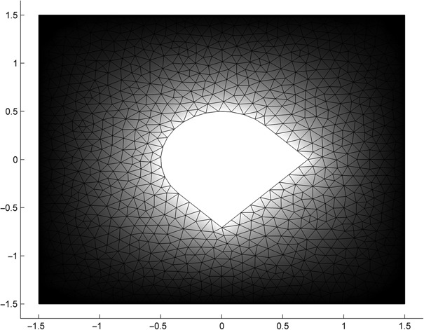
FIGURE 14.9 Voltage distribution of struct14_3.geo.
Calling the Matlabfunction get_tri2d_E.m at the end of fem_2d_1.m results in Figure 14.10, the electric field magnitude distribution of struct14_3.geo. The calculation of the electric field is identical to this calculation in get_tri2d_cap.m and there would have been some programming efficiency in including the electric field calculation and graphics generation into this latter function. MATLAB program get_tri2d_E.m — showing the electric field profile — is written as a separate function only for the convenience of the reader:
function get_tri2d_E(v, nr_nodes, nr_trs, nds, trs)
% Calculate and show the field magnitude profile
% E_mag calculation is identical to that in capacitance calculation
% function
 eps0 = 8.854;
 d = ones(3,3); E_mag = zeros(nr_trs,1); Ex = E_mag; Ey = E_mag;
 for tri = 1 : nr_trs
  n1 = trs(1,tri); n2 = trs(2,tri); n3 = trs(3,tri);
  d(1,2) = nds.x(n1); d(1,3) = nds.y(n1);
  d(2,2) = nds.x(n2); d(2,3) = nds.y(n2);
  d(3,2) = nds.x(n3); d(3,3) = nds.y(n3);
  temp = (d[1; 0; 0]); b1 = temp(2); c1 = temp(3);
  temp = (d[0; 1; 0]); b2 = temp(2); c2 = temp(3);
  temp = (d[0; 0; 1]); b3 = temp(2); c3 = temp(3);
  E_x(tri) = v(n1)*b1 + v(n2)*b2 + v(n3)*b3;
  E_y(tri) = v(n1)*c1 + v(n2)*c2 + v(n3)*c3;
  E_mag(tri) = E_x(tri).^2 + E_y(tri).^2;
 end
 E_peak = sqrt(max(E_mag))
 E_mag = sqrt(E_mag/max(E_mag)); % normalize
 E_x = abs(E_x)/max(E_x);
 E_y = abs(E_y)/max(E_y);
 E_show = E_mag; % pick E_x, E_y or E_mag to display
 figure(3)
 x_min = min(nds.x)*1.1;
 if x_min == 0, x_min = -.5; end;
 x_max = max(nds.x)*1.1;
 y_min = min(nds.y)*1.1;
 if y_min == 0, y_min = -.5; end;
 y_max = max(nds.y)*1.1; axis ([x_min, x_max, y_min, y_max]);
 axis ([x_min, x_max, y_min, y_max]);
 axis square;
 hold on
 for tri = 1 : nr_trs
  n1 = trs(1,tri); n2 = trs(2,tri); n3 = trs(3,tri);
  x = [nds.x(n1); nds.x(n2); nds.x(n3)];
  y = [nds.y(n1); nds.y(n2); nds.y(n3)];
  E = [E_show(tri); E_show(tri); E_show(tri)];
  colormap (gray) % Delete this line for color graphics
  fill(x,y,E)
 end
end
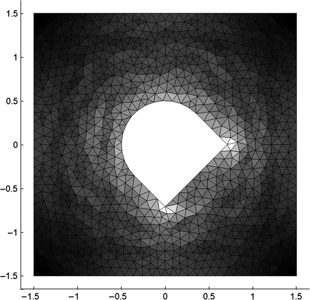
FIGURE 14.10 Electric field magnitude profile for structure shown in struct14_3.geo.
Figure 14.10 shows the electric field magnitude profile produced by get_tri2d_E.m. Once again, the color figure produced on a computer display allows more insight than the black-and-white text rendition. In either case, it is clear that the electric field peaks at the sharp corners of the structure. Modifying get_tri2d_E.m to show field components, to tabulate field values, and so on, is very straightforward.
14.6 Multiple Electrodes
(Note: This section relies heavily on the results of Chapter 10. The electrostatic concepts and circuital analysis of a multiple electrode structure are the same regardless of whether FD or FEM analysis is utilized to find the parameters of the structure. Even if the reader has no interest in FD analysis, reading Chapter 10 before reading this section is recommended.)
The gmsh file struct14_4.geo describes a simple rectangular two-electrode structure.
// Gmsh structure file struct14_4.geo
lc = .1;
// exterior loop
Point(1) = {-2, -1.5, 0, lc};
Point(2) = {2, -1.5, 0, lc};
Point(3) = {2, 1.5, 0, lc};
Point(4) = {-2, 1.5, 0, lc};
Line(1) = {1, 2};
Line(2) = {2, 3};
Line(3) = {3, 4};
Line(4) = {4, 1};

// interior surface which will become a hole
Point(5) = {-1, -.7, 0, lc};
Point(6) = {-.2, -.8, 0, lc};
Point(7) = {-.2, .45, 0, lc};
Point(8) = {-1, .5, 0, lc};
Line(105) = {5, 6};
Line(106) = {6, 7};
Line(107) = {7, 8};
Line(108) = {8, 5};

Line Loop(1) = {105, 106, 107, 108};
Plane Surface(200) = {1};

// second inner surface
Point(15) = {0., -.5, 0, lc};
Point(16) = {1, -.5, 0, lc};
Point(17) = {.8, .5, 0, lc};
Point(18) = {.2, .5, 0, lc};
Line(115) = {15, 16};
Line(116) = {16, 17};
Line(117) = {17, 18};
Line(118) = {18, 15};

Line Loop(2) = {115, 116, 117, 118};
Plane Surface(210) = {2};

// exterior surface
Line Loop(3) = {1, 2, 3, 4};
Plane Surface(4) = {3, 1, 2} ;
The structure described by struct14_4.geo is shown in Figure 14.11.
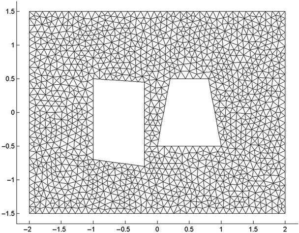
FIGURE 14.11 Two-electrode structure described by struct 14_14.geo.
In this structure, two obviously different, nontouching, electrodes are contained in the same outer boundary. File struct14_4.geo defines both of these electrodes as excluded regions inside the outer boundary. The left-hand electrode is bounded by lines 105–108; the right-hand electrode, by lines 115–118.
The following questions might be posed:
- What are the various capacitances of this structure?
- If the left-hand electrode (electrode 1) is set as a boundary condition while the right-hand electrode (electrode 2) is left floating, what voltage will it float to?
As described in Chapter 10, these questions may be answered using a circuit model of the system. Figure 10.1 shows the three-capacitor model that describes this system.
If we set both electrodes to 1 V (by setting the boundary condition on lines 105–108 and lines 115–118 = 1), we find that fem_2d_1.m calculates Ca = the sum of C1 and C2 = 75.66 pF/m.
If we set electrode 1 to 1 V and electrode 2 to 0 V by setting only lines 105–108 = 1 V, then lines 115–118 remain at 0 V by default, and we calculate Ca = the sum of C 1 and C 12 = 85.98 pF/m.
If we set electrode 2 to 1 V and electrode 1 to 0 V, we calculate Cb = the sum of C 2 and C 12 = 77.43 pF/m.
Equations (10.4), (10.5), and (10.6) invert these relationships and give us the capacitance values C 1 = 42.1, C 2 = 33.6, and C 12 = 43.9 pF/m, respectively.
If we set electrode 1 to 1 V and let electrode 2 float, then (again referring to the derivation in Chapter 10), we obtain
As described in Chapter 10, the voltage distribution resulting from the first FEM calculation above is identically the sum of the voltage distributions of the the last two FEM calculations above, and this relationship may be used to eliminate one FEM calculation.
Utilization of a symmetric structure as described in Chapter 10 to eliminate one FEM calculation is also a valid option. Since we are using unstructured grids for the FEM calculation, however, we have no a priori guarantee that the latter two FEM calculations above will yield identical results, even though we are using a symmetric structure. In this case the calculation that yields the lower capacitance is the more accurate one, but we have no way of knowing which calculation will yield the lower capacitance until we do both calculations, and at that point there is no longer any value in “eliminating” one calculation because both calculations have already been done — we simply choose the lower result to use in both cases.
Problems
14.1 Modify get_tri2d_E.m so that it can display Ex and Ey as well as Emag. Show these results for struct14_4 with the right electrode set to 1 V and the left electrode set to 0 V.
14.2 Write a MATLAB function that takes the voltage profile from a fem2d_1.m run and creates a graph of equipotential contours.
14.3 Create a gmsh structure file (xxx.geo) for two concentric squares of sides 2 and 4. Mesh the inner region finer than the outer region. Rotate the inner square in 5o steps; create the mesh and the boundary conditions, and then find the capacitance and peak electric field magnitude as a function of the rotation angle.
14.4 Using any text editor, edit the boundary condition file of the previous example (at 0 rotation) and remove all entries for the right-hand wall of the outer square. (Re)run the FEM analysis and comment on the capacitance and voltage distribution as compared to the previous results. (Hint: This strategy will be formally presented in Chapter 15.)
References
- 1. C. Geuzaine and J. F. Remacle, Gmsh: A three-dimensional finite element mesh generator with built-in pre- and post-processing facilities, Int. J. Num. Methods Eng., 79(11): 1309–1331 (2009).
- 2.
http://geuz.org/gmsh/doc/LICENSE.txt - 3.
http://www.ideaconsulting.com/strip.htm