4.3.1 Exponentially speaking

The exponential function descends to an asypmtote at 0 with a rate dependent on the positive parameter alpha. Thus the function

4.2

has a root at

4.3

For small alpha, the root will be large, as the function will be very “flat” as it crosses zero. For alpha moderate to large, the function will be very rapidly changing as it crosses the -axis near . This problem provides a simple example of some of root-finding and a quite good test of software. Of course, we already have the answer and can see it clearly if we draw the function and also draw a line for -axis. Let us look at the cases and . The function is drawn in dashed and dotted, respectively, by the code that follows. Note that an attempt to find a root in an interval where the end points do not have function values with different signs gives an error (Figure 4.1).

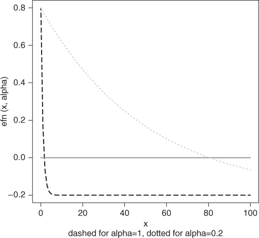
cat("exponential example
")
## exponential example
require("rootoned")
alpha <- 1
efn <- function(x, alpha) {
    exp(-alpha * x) - 0.2
}
zfn <- function(x) {
    x * 0
}
tint <- c(0, 100)
curve(efn(x, alpha = 1), from = tint[1], to = tint[2], lty = 2, ylab = "efn(x, alpha)")
title(sub = "Dashed for alpha = 1, dotted for alpha = 0.2")
curve(zfn, add = TRUE)
curve(efn(x, alpha = 0.02), add = TRUE, lty = 3)
rform1 <- -log(0.2)/1
rform2 <- -log(0.2)/0.02
resr1 <- uniroot(efn, tint, tol = 1e-10, alpha = 1)
cat("alpha = ", 1, "
")
## alpha =  1
cat("root(formula)=", rform1, "  root1d:", resr1$root, " tol=", resr1$estim.prec,
    "  fval=", resr1$f.root, "  in   ", resr1$iter, "

")
## root(formula)= 1.609   root1d: 1.609  tol= 0.0005702   fval= 0   in    13
resr2 <- uniroot(efn, tint, tol = 1e-10, alpha = 0.02)
cat("alpha = ", 0.02, "
")
## alpha =  0.02
cat("root(formula)=", rform2, "  root1d:", resr2$root, " tol=", resr2$estim.prec,
    "  fval=", resr2$f.root, "  in   ", resr2$iter, "

")
## root(formula)= 80.47  root1d: 80.47 tol= 5.004e-11  fval= 9.381e-15  in  8
cat("
")

cat("Now look for the root in [0,1]
")
## Now look for the root in [0,1]
tint2a <- c(0, 1)
resr2a <- uniroot(efn, tint2a, tol = 1e-10, alpha = 0.02)
## Error: f() values at end points not of opposite sign

4.3.2 A normal concern

The problem we will now consider is actually one of finding the maximum of a one-dimensional problem, the subject of a related chapter. Its relevance to the root-finding problem is how it illustrates the difficulties that numeric precision can introduce.

Consider the Gaussian (normal) density function

4.4

This is the usual “bell-shaped” curve. It is always positive, and we want to find its maximum. Obviously, we know the answer—the mean . As we are discussing root-finding, we will look at the derivative with respect to . This function can be found using R with the D() or deriv() tools, which we will explore in Chapter 5.

The function we want to use is

4.5

Let us set mu = 4 and draw the function from 0 to 8 for (in gray) and (Figure 4.2). To keep the graph viewable, we the log of the magnitudes but keep the sign. As the standard deviation sigma gets smaller, the function gets steeper.

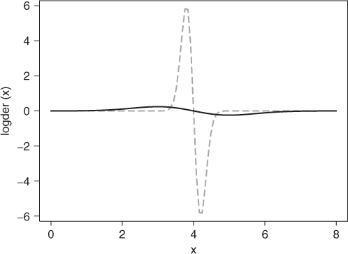
Let us use 2 and 6 as the limits of our search interval and find the root for progressively smaller.

cat("Gaussian derivative
")
## Gaussian derivative
der <- function(x, mu, sigma) {
    dd <- (-1) * (1/sqrt(2 * pi * sigma^2))*(exp(-(x - mu)^2/(2 * sigma^2)) *
        ((x - mu)/(sigma^2)))
}
r1 <- uniroot(der, lower = 1, upper = 6, mu = 4, sigma = 1)
r.1 <- uniroot(der, lower = 1, upper = 6, mu = 4, sigma = 0.1)
r.01 <- uniroot(der, lower = 1, upper = 6, mu = 4, sigma = 0.01)
r.001 <- uniroot(der, lower = 1, upper = 6, mu = 4, sigma = 0.001)
sig <- c(1, 0.1, 0.01, 0.001)
roo <- c(r1$root, r.1$root, r.01$root, r.001$root)
tabl <- data.frame(sig, roo)
print(tabl)
##     sig roo
## 1 1.000   4
## 2 0.100   4
## 3 0.010   1
## 4 0.001   1

What is going on here?! We know the root should be at 4, but in the final two cases, it is at 1. The reason turns out to be that the function value at is computationally zero—a root. The danger is that we just do not recognize that this is not the “root” we likely wish to find, for example, if we are using the derivative as a way to sharpen the finding of a peak on a spectrometer.

Fortunately, thanks to Martin Maechler, there is the package Rmpfr (Maechler, 2013) that allows us to use extended precision arithmetic. This will also work with many R functions, but not with tools such as uniroot() that are programmed in languages other than R. However, when I learned of this issue at the 2011 UseR! meeting, I spent some time in one of the sessions that did not overlap my interests in coding an R version of the root-finder (zeroin() in the developmental R-forge package rootoned from project optimizer). Martin included a modified version of this as unirootR() in Rmpfr. This shows quite clearly that there is no root at 1.

Unfortunately, the code to present this example could not be run in the knitr environment that generated much of this book. (We are still trying to discover the reason.) Thus the computations were carried out in the R terminal and the results are copied here.

> require(Rmpfr)
> der<-function(x,mu,sigma){
+     dd<-(-1)*(1/sqrt(2 * pi * sigma^2)) * (exp(-(x - mu)^2/(2 * sigma^2)) *
+     ((x - mu)/(sigma^2)))
+ }
> rootint1<-mpfr(c(1.9, 2.1),200)
> rootint1
2 'mpfr' numbers of precision  200   bits
[1] 1.899999999999999911182158029987476766109466552734375
[2] 2.100000000000000088817841970012523233890533447265625
> r140<-try(unirootR(der, rootint1, tol=1e-40, mu=4, sigma=1))
> # r140
> rootint2<-mpfr(c(1, 6),200)
> rootint2
2 'mpfr' numbers of precision  200   bits
[1] 1 6
> r140a<-try(unirootR(der, rootint2, tol=1e-40, mu=4, sigma=1))
> r140a
$root
1 'mpfr' number of precision  200   bits
[1] 3.9999999999999999999999999999999999999999999999422505411069977
$f.root
1 'mpfr' number of precision  200   bits
[1] 2.3038700822723117720200096647152975711858994581054996741312416e-47
$iter
[1] 8
$estim.prec
[1] 5e-41
$converged
[1] TRUE

4.3.3 Little Polly Nomial

Polynomial roots are a common problem that should generally be solved by methods different from those where our goal is to find a single real root of a real scalar function of one variable. This is easily illustrated by an example. Suppose we want the roots of the polynomial

4.6

This has the set of coefficients that we would establish using the R code

 z <- c(10, -3, 0, 1)

The package polynom solves this easily using polyroot(z).

z <- c(10, -3, 0, 1)
simpol <- function(x) {
    # calculate polynomial z at x
    zz <- c(10, -3, 0, 1)
    ndeg <- length(zz) - 1  # degree of polynomial
    val <- zz[ndeg + 1]
    for (i in 1:ndeg) {
        val <- val * x + zz[ndeg + 1 - i]
    }
    val
}
tint <- c(-5, 5)
cat("roots of polynomial specified by ")
## roots of polynomial specified by
print(z)
## [1] 10 -3  0  1
require(polynom)
allroots <- polyroot(z)
print(allroots)
## [1]  1.3064+1.4562i -2.6129+0.0000i  1.3064-1.4562i
cat("single root from uniroot on interval ", tint[1], ",", tint[2], "
")
## single root from uniroot on interval  -5 , 5
rt1 <- uniroot(simpol, tint)
print(rt1)
## $root
## [1] -2.6129
##
## $f.root
## [1] 2.5321e-06
##
## $iter
## [1] 9
##
## $estim.prec
## [1] 6.1035e-05

Here we see that uniroot does a perfectly good job of finding the real root of this cubic polynomial. It will not, however, solve the simple polynomial

4.7

because both the roots are at 4 and the function never crosses the -axis. uniroot() insists on having a starting interval where the function has opposite sign at the ends of the interval. uniroot() should (and in our example below does) work when there is a root with odd multiplicity, so that there is a crossing of the axis.

z <- c(16, -8, 1)
simpol2 <- function(x) {
    # calculate polynomial z at x
    val <- (x - 4)^2
}
tint <- c(-5, 5)
cat("roots of polynomial specified by ")
## roots of polynomial specified by
print(z)
## [1] 16 -8  1
require(polynom)
allroots <- polyroot(z)
print(allroots)
## [1] 4+0i 4-0i
cat("single root from uniroot on interval ", tint[1], ",", tint[2], "
")
## single root from uniroot on interval  -5 , 5
rt1 <- try(uniroot(simpol2, tint), silent = TRUE)
print(strwrap(rt1))
## [1] "Error in uniroot(simpol2, tint) : f() values at end points not of"
## [2] "opposite sign"
cat("
 Try a cubic
")
##
##  Try a cubic
cub <- function(z) {
    val <- (z - 4)^3
}
cc <- c(-64, 48, -12, 1)
croot <- polyroot(cc)
croot
## [1] 4-0i 4+0i 4+0i
ans <- uniroot(cub, lower = 2, upper = 6)
ans
## $root
## [1] 4
##
## $f.root
## [1] 0
##
## $iter
## [1] 1
##
## $estim.prec
## [1] 2

4.3.4 A hypothequial question

In Canada, mortgages fall under the Canada Interest Act. This has an interesting clause:

6. Whenever any principal money or interest secured by mortgage of real estate is, by the mortgage, made payable on the sinking fund plan, or on any plan under which the payments of principal money and interest are blended, or on any plan that involves an allowance of interest on stipulated repayments, no interest whatsoever shall be chargeable, payable, or recoverable, on any part of the principal money advanced, unless the mortgage contains a statement showing the amount of such principal money and the rate of interest thereon, calculated yearly or half-yearly, not in advance.

This clause allowed the author to charge rather a high fee to recalculate the payment schedule for a private lender who had, in a period when the annual rate of interest was around 20% in the early 1980s, used a US computer program. The borrower wanted to make monthly payments. This is feasible in Canada, but we must do the calculations with a rate that is equivalent to the half-yearly rate. So if the annual rate is %, the semiannual rate is %, and we want compounding at a monthly rate that is equal to this semiannual rate. That is,

4.8

and our root-finding problem is the solution of

4.9

We can actually write down a solution, of course, as

4.10

A textbook (and possibly dangerous) approach to this has been to plug this formula into a spreadsheet or other system (including R). The difficulty is that approximations to the fractional (1/6) power are just that, approximations. And the answer for low interest rates are bound to give digit cancellation when we subtract 1 from the (1/6) root of a number not very different from 1. However, R does, in fact, a good job. Using uniroot on the function above is also acceptable if the tolerance is specified and small, otherwise we get a rather poor answer.

A quite good way to solve this problem is by means of the binomial theorem, where the expansion of (substituting for ) is

4.11

Besides converging very rapidly, this series expansion begins with 1, which we can subtract analytically, thereby avoiding digit cancellation. The following calculations present the ideas in program form, which show that any of the three approaches are reasonable for this problem.

mrate <- function(R) {
    val <- 0
    den <- 1
    fact <- 1/6
    term <- 1
    rr <- R/200
    repeat {
        # main loop
        term <- term * fact * rr/den
        vallast <- val
        val <- val + term
        # cat('term =',term,' val now ',val,'
')
        if (val == vallast)
            break
        fact <- (fact - 1)
        den <- den + 1
        if (den > 1000)
            stop("Too many terms in mrate")
    }
    val * 100
}
A <- function(I, Rval) {
    A <- (1 + I/100)^6 - (1 + R/200)
}
Rvec <- c()
i.formula <- c()
i.root <- c()
i.mrate <- c()
for (r2 in 0:18) {
    R <- r2/2  # rate per year
    Rvec <- c(Rvec, R)
    i.formula <- c(i.formula, 100 * ((1 + R/200)^(1/6) - 1))
    i.root <- c(i.root, uniroot(A, c(0, 20), tol = .Machine$double.eps, Rval = R)$root)
    i.mrate <- c(i.mrate, mrate(R))
}
tabR <- data.frame(Rvec, i.mrate, (i.formula - i.mrate), (i.root - i.mrate))
colnames(tabR) <- c("rate", "i.mrate", "form - mrate", "root - mrate")
print(tabR)
##    rate  i.mrate form - mrate root - mrate
## 1   0.0 0.000000   0.0000e+00   0.0000e+00
## 2   0.5 0.041623  -3.1572e-15   7.8132e-15
## 3   1.0 0.083160   4.7323e-15  -6.3144e-15
## 4   1.5 0.124611  -5.1625e-15   5.7038e-15
## 5   2.0 0.165976   5.5511e-16   3.3307e-16
## 6   2.5 0.207256   9.9920e-16   2.6923e-15
## 7   3.0 0.248452   5.1625e-15  -5.8287e-15
## 8   3.5 0.289562   1.6653e-16  -2.1094e-15
## 9   4.0 0.330589   3.7192e-15  -7.2164e-15
## 10  4.5 0.371532  -6.8279e-15   4.1078e-15
## 11  5.0 0.412392  -3.7192e-15   7.1054e-15
## 12  5.5 0.453168   7.6605e-15  -3.2196e-15
## 13  6.0 0.493862  -9.5479e-15   1.1657e-15
## 14  6.5 0.534474   5.5511e-15  -5.3291e-15
## 15  7.0 0.575004  -1.3323e-15  -5.8842e-15
## 16  7.5 0.615452  -5.3291e-15   5.3291e-15
## 17  8.0 0.655820   6.8834e-15  -3.9968e-15
## 18  8.5 0.696106  -8.5487e-15   2.2204e-15
## 19  9.0 0.736312   1.1102e-15  -9.5479e-15

References

- Brent R 1973 Algorithms for Minimization without Derivatives. Prentice-Hall, Englewood Cliffs, NJ.
- Maechler M 2013 Rmpfr: R MPFR - Multiple Precision Floating-Point Reliable. R package version 0.5-3.
- Nash JC 1979 Compact Numerical Methods for Computers: Linear Algebra and Function Minimisation. Hilger, Bristol.