
Chapter 14
Applications of mathematical programming
Mathematical programming is, in my view, satisfaction of constraints with an attempt to minimize or maximize an objective function. That is, there are “many” constraints and they are the first focus of our attention. Moreover, the subject has been driven by a number of practical-resource-assignment problems, so the variables may also be integers instead of or as well as real numbers.
14.1 Statistical applications of math programming
In this field, R shows its statistical heritage and is not at the forefront. Most statisticians do not use math programming. I include myself in this. My needs for such tools have largely been driven by approximation problems where we wish to minimize the sum of absolute errors or the maximum absolute error. There are also situations where I have wanted to solve some optimization problems such as the diet problem, where the constraints are the required total intake of nutrients or limits on salt and fats and the objective is to minimize the cost to provide the diet.
In the 1980s, the University of New South Wales ran a program directed by Bruce Murtagh to offer companies student help with optimization problems at bargain consulting prices. I believe that $5000 was paid by a cat food company to determine an economical blend for tinned pet food. The resulting mixture, determined from a linear program, used ground up fish heads and fish oil with mostly grain components for a saving many times the consulting fee. This is not the sort of problem R users generally solve.
There are, however, some applications to statistics. One area is that of obfuscating published statistics to render difficult or impossible the retrieval of private information by subtraction from totals. See, for example, the Statistics Canada report “Data Quality and Confidentiality Standards and Guidelines (Public): 2011 Census Dissemination” (http://www12.statcan.gc.ca/census-recensement/2011/ref/DQ-QD/2011_DQ-QD_Guide_E.pdf). Gordon Sande presents some ideas on this in a paper to the 2003 conference of the (US) Federal Committee on Statistical Methodology (http://www.fcsm.gov/events/papers2003.html). The idea is to use constraints to keep published data far enough from actual figures to inhibit the revelation of individual data by calculation, while minimizing the perturbations in some way. Another use of math programming in large statistical agencies is presented by McCarthy and Bateman (1988) who consider the design of surveys. Bhat (2011) presents a quite good overview of math programming in statistics in his doctoral thesis introduction, listing some applications in contingency tables and hypothesis testing as well as the minimax and least absolute deviations problems that I mentioned earlier. There are also some applications in machine learning, for example, http://stackoverflow.com/questions/12349122/solving-quadratic-programming-using-r.
14.2 R packages for math programming
We have already dealt with the general nonlinear programming problem in Chapter 13. However, my experience has been that despite the formal statement of the problem—minimize a nonlinear objective subject to possibly nonlinear constraints—is the generalization of traditional linear and quadratic programming problems of this chapter, many problems have rather few constraints. They are constrained nonlinear function minimization problems.
In Chapter 13, we considered both alabama (Varadhan, 2012) and Rsolnp (Ghalanos and Theussl, 2012). These packages require, in my view, more care and attention to use than most discussed in this book. Rsolnp is the only package that is listed in the R-forge project “Integer and Nonlinear Optimization in R (RINO)”, but there are three other packages in the code repository. However, none of these has been updated in ![]() years before the time of writing, while
years before the time of writing, while Rsolnp appears to be maintained. Because the packages in this paragraph have more kinship with function minimization, we will not address them further in this chapter.
Most traditional math programming involves some special form of objective or constraints, in particular linear constraints with either a linear or a quadratic objective. This leads to the well-established linear programming (LP) and quadratic programming problems.
Quadratic programming has two tools as the main candidates in R. Solve.QP() from package quadprog (original by Berwin A. Turlach R port by Andreas Weingessel, 2013) has to my eyes the more traditional interface, while ipop() from package kernlab (Karatzoglou et al. 2004) requires a somewhat unusual format for specifying the linear constraints.
For linear programming, packages linprog (Henningsen, 2012) and lpSolve (Berkelaar et al. 2013) have slightly different calling sequences. Both of these are for real variables. However, much of LP is for integer or mixed-integer variables. The package Rglpk (Theussl and Hornik, 2013) provides an interface to the Gnu LP kit and can handle both real- and mixed-integer problems. The same authors provide Rsymphony (Harter et al. 2013) and ROI (Hornik et al. 2011) for mixed-integer programming problems. These are allquite complicated packages, with a style for inputting a problem that is quite different from the problem statements we have seen elsewhere in this book.
Similarly, Jelmer Ypma of the University College London offers interfaces nloptr to Steven Johnson's NLopt and ipoptr to the COIN-OR interior point optimizer(s) ipopt(). (This should not be confused with ipop() from kernlab.) These are not part of the CRAN repository and like the tools of the previous paragraph require installation in a way that is not common with other R packages. I have decided not to discuss either set of tools as I have not had enough experience with them to comment fairly. However, it is important to note that interior point methods have been much discussed in the optimization literature over the past two decades, and there is no mainstream R package that addresses the need. Nor does R appears to offer any tool for convex optimization at the time of writing.
There are also R interfaces to some commercial solvers. Rcplex is an interface to the CPLEX optimization engine. The history of this suite of solvers is described in http://en.wikipedia.org/wiki/CPLEX. The R interface appears to support only Linux platforms. Similarly, Rmosek (http://rmosek.r-forge.r-project.org/) is an R interface to the MOSEK solvers and claims to deal with large-scale optimization problems having linear, quadratic, and some other objectives with integer constraints. Again, installation will be nonstandard because the user must first install the commercial package. I have no experience with such packages and will not provide a treatment here.
There are R packages that build on some of the tools above. For example, package parma for “Portfolio Allocation and Risk Management Applications” calls the Rgplk tools. In the rest of this chapter, we will look at using some of them for some illustrative problems of a statistical nature.
14.3 Example problem: L1 regression
Traditional regression estimation problems minimize the sum of squared residuals. However, there are many arguments in favor of other loss functions based on the residuals (L-infinity or minimax regression, M-estimators, and others). Here we will look at L1 or least absolute deviations (LAD) regression. For a linear model, this is stated as
where ![]() is the matrix of predictor variables (generally one column is all 1's to provide a constant or intercept term) and
is the matrix of predictor variables (generally one column is all 1's to provide a constant or intercept term) and ![]() is the independent or predicted variable. Instead of minimizing the sum of squared residuals, we are minimizing the sum of absolute values.
is the independent or predicted variable. Instead of minimizing the sum of squared residuals, we are minimizing the sum of absolute values.
Let us set up a small problem.
x <- c(3, -2, -1)
a1 <- rep(1, 10)
a2 <- 1:10
a3 <- a2^2
A <- matrix(c(a1, a2, a3), nrow = 10, ncol = 3)
A
##       [,1] [,2] [,3]
##  [1,]    1    1    1
##  [2,]    1    2    4
##  [3,]    1    3    9
##  [4,]    1    4   16
##  [5,]    1    5   25
##  [6,]    1    6   36
##  [7,]    1    7   49
##  [8,]    1    8   64
##  [9,]    1    9   81
## [10,]    1   10  100
## create model data
y0 = A %*% x
y0
##       [,1]
##  [1,]    0
##  [2,]   −5
##  [3,]  −12
##  [4,]  −21
##  [5,]  −32
##  [6,]  −45
##  [7,]  −60
##  [8,]  −77
##  [9,]  −96
## [10,] −117
## perturb the model data --- get working data
set.seed(1245)
y <- as.numeric(y0) + runif(10, -1, 1)
y
##  [1]    0.324886   −4.428305  −12.854561  −20.393083
##  [5]  −32.854574  −45.193280  −60.690202  −77.243728
##  [9]  −96.406035 −117.241829
## try a least squares model
l2fit <- lm(y ∼ a2 + a3)
l2fit
##
## Call:
## lm(formula = y ∼ a2 + a3)
##
## Coefficients:
## (Intercept)           a2           a3
##       3.737       −2.339       −0.976
It turns out that our regular optimizers get into trouble solving this in the L1 norm. We also check the L2 or square norm solution, which turns out to be much less trouble.
sumabs <- function(x, A, y) {
    # loss function
    sum(abs(y - A %*% x))
}
sumsqr <- function(x, A, y) {
    # loss function
    sum((y - A %*% x)^2)  # a poor way to do this
}
require(optimx)
st <- rep(1, 3)
ansL1 <- optimx(st, sumabs, method = "all", control = list(usenumDeriv = TRUE), A = A, y = y)
## Warning: Replacing NULL gr with 'numDeriv' approximation
## Warning: bounds can only be used with method L-BFGS-B (or Brent)
## Warning: bounds can only be used with method L-BFGS-B (or Brent)
## Warning: bounds can only be used with method L-BFGS-B (or Brent)
print(summary(ansL1, order = value))
##                   p1        p2        p3        value
## nmkb        3.605201 −2.302050 −0.978265  3.29511e+00
## nlm         3.582684 −2.277278 −0.980520  3.29524e+00
## ucminf      3.545880 −2.236248 −0.984252  3.29539e+00
## hjkb        3.490341 −2.175003 −0.989822  3.29551e+00
## Rvmmin      3.604006 −2.290916 −0.979367  3.30003e+00
## nlminb      3.509092 −2.210676 −0.986442  3.31376e+00
## bobyqa      3.418332 −2.049762 −1.004648  3.77613e+00
## BFGS        0.352885 −1.263250 −1.054194  7.07201e+00
## CG          0.352885 −1.263250 −1.054194  7.07201e+00
## Nelder-Mead 0.352885 −1.263250 −1.054194  7.07201e+00
## L-BFGS-B    0.352885 −1.263250 −1.054194  7.07201e+00
## newuoa      0.427852 −0.821233 −1.104232  9.20869e+00
## Rcgmin      0.902925  0.542689 −1.288875  2.50204e+01
## spg               NA        NA        NA 8.98847e+307
##             fevals gevals niter convcode  kkt1  kkt2 xtimes
## nmkb           257     NA    NA        0 FALSE  TRUE  0.032
## nlm             NA     NA    29        0 FALSE FALSE  0.004
## ucminf          51     51    NA        0 FALSE FALSE  0.008
## hjkb          6764     NA    19        0 FALSE  TRUE  0.108
## Rvmmin         142     20    NA        0 FALSE FALSE  0.012
## nlminb          54     22    22        1 FALSE FALSE  0.004
## bobyqa         206     NA    NA        0 FALSE FALSE  0.004
## BFGS           146    146    NA        0 FALSE FALSE  0.016
## CG             146    146    NA        0 FALSE FALSE  0.012
## Nelder-Mead    146    146    NA        0 FALSE FALSE  0.016
## L-BFGS-B       146    146    NA        0 FALSE FALSE  0.016
## newuoa         302    NA     NA        0 FALSE  TRUE  0.004
## Rcgmin        1011    112    NA        1 FALSE FALSE  0.036
## spg             NA     NA    NA     9999    NA    NA  0.160
ansL2 <- optimx(st, sumsqr, method = "all", control = list(usenumDeriv = TRUE), A = A, y = y)
## Warning: Replacing NULL gr with 'numDeriv' approximation
## Warning: bounds can only be used with method L-BFGS-B (or Brent)
## Warning: bounds can only be used with method L-BFGS-B (or Brent)
## Warning: bounds can only be used with method L-BFGS-B (or Brent)
print(summary(ansL2, order = value))
##                  p1       p2        p3        value fevals
## Rvmmin      3.73671 −2.33884 −0.975874  1.91298e+00     92
## nlm         3.73671 −2.33884 −0.975874  1.91298e+00     NA
## ucminf      3.73671 −2.33884 −0.975874  1.91298e+00     10
## nlminb      3.73671 −2.33884 −0.975874  1.91298e+00      9
## BFGS        3.73671 −2.33884 −0.975874  1.91298e+00     18
## CG          3.73671 −2.33884 −0.975874  1.91298e+00     18
## Nelder-Mead 3.73671 −2.33884 −0.975874  1.91298e+00     18
## L-BFGS-B    3.73671 −2.33884 −0.975874  1.91298e+00     18
## Rcgmin      3.73671 −2.33884 −0.975874  1.91298e+00   1007
## newuoa      3.73671 −2.33884 −0.975874  1.91298e+00    273
## bobyqa      3.73670 −2.33884 −0.975874  1.91298e+00    612
## hjkb        3.73667 −2.33882 −0.975876  1.91298e+00   2600
## nmkb        3.73648 −2.33865 −0.975894  1.91298e+00    150
## spg              NA       NA        NA 8.98847e+307     NA
##             gevals niter convcode  kkt1 kkt2 xtimes
## Rvmmin          19    NA        0  TRUE TRUE  0.000
## nlm             NA    10        0  TRUE TRUE  0.000
## ucminf          10    NA        0  TRUE TRUE  0.000
## nlminb           8     7        0  TRUE TRUE  0.000
## BFGS            18    NA        0  TRUE TRUE  0.000
## CG              18    NA        0  TRUE TRUE  0.004
## Nelder-Mead     18    NA        0  TRUE TRUE  0.004
## L-BFGS-B        18    NA        0  TRUE TRUE  0.000
## Rcgmin         149    NA        1  TRUE TRUE  0.040
## newuoa          NA    NA        0  TRUE TRUE  0.004
## bobyqa          NA    NA        0  TRUE TRUE  0.008
## hjkb            NA    19        0  TRUE TRUE  0.040
## nmkb            NA    NA        0 FALSE TRUE  0.016
## spg             NA    NA     9999    NA   NA  0.164
## l2fit sum of squares
sumsqr(coef(l2fit), A, y)
## [1] 1.91298
We can, however, use LP to solve the LAD problem in ![]() observations and
observations and ![]() parameters as defined by the
parameters as defined by the ![]() matrix and
matrix and ![]() vector above. Following the treatment in Bisschop and Roelofs (2006), we establish the problem as a minimization of
vector above. Following the treatment in Bisschop and Roelofs (2006), we establish the problem as a minimization of
subject to the constraints
These strange-looking constraints, imposed simultaneously, push the sum of absolute residuals to the minimum.
Unfortunately, most LP solvers automatically impose nonnegativity constraints on the ![]() variables that we wish to find. We work around this by defining
variables that we wish to find. We work around this by defining
where the ![]() and
and ![]() variables are nonnegative. Furthermore, the solver we will call here,
variables are nonnegative. Furthermore, the solver we will call here, SolveLP() from package linprog, prefers the constraints to be as ![]() rather than
rather than ![]() forms. To make this work, we build a supermatrix
forms. To make this work, we build a supermatrix

The right-hand side of the constraints is then the vector (bvec)
and the objective function is defined by a vector (cvec) that has ![]() ones and
ones and ![]() zeros. The latter elements are used to define the
zeros. The latter elements are used to define the ![]() and
and ![]() elements of our solution, while the ones are to give us the objective function.
elements of our solution, while the ones are to give us the objective function.
This setup is captured in the following function, called LADreg, which takes as input the matrix ![]() and the vector
and the vector ![]() .
.
LADreg <- function(A, y) {
    # Least sum abs residuals regression
    require(linprog)
    m <- dim(A)[1]
    n <- dim(A)[2]
    if (length(y) != m)
        stop("Incompatible A and y sizes in LADreg")
    ones <- diag(rep(1, m))
    Abig <- rbind(cbind(-ones, -A, A), cbind(-ones, A, -A))
    bvec <- c(-y, y)
    cvec <- c(rep(1, m), rep(0, 2 * n))  # m z's, n pos x, n neg x
    ans <- solveLP(cvec, bvec, Abig, lpSolve = TRUE)
    sol <- ans$solution
    coeffs <- sol[(m + 1):(m + n)] - sol[(m + n + 1):(m + 2 * n)]
    names(coeffs) <- as.character(1:n)
    res <- as.numeric(sol[1:m])
    sad <- sum(abs(res))
    answer <- list(coeffs = coeffs, res = res, sad = sad)
}
Let us use this to solve our example problem.
myans1 <- LADreg(A, y)
myans1$coeffs
##         1         2         3
##  3.489517 −2.174797 −0.989834
myans1$sad
## [1] 3.2951
It turns out that there are tools in R that are more specifically intended for this problem. In particular, L1linreg() from package pracma and rq() from quantreg can do the job. quantreg (Koenker, 2013) also has a nonlinear quantile regression function nlrq(). Koenker (2005) has a large presence in the area of quantile regression and his package is well established and can be recommended for this application. The ad hoc treatment above is intended to provide an introduction to how similar problems can be approached with available tools.
require(pracma)
ap1 <- L1linreg(A = A, b = y)
ap1
## $x
## [1]  3.605010 −2.301839 −0.978285
##
## $reltol
## [1] 2.41727e-08
##
## $niter
## [1] 20
sumabs(ap1$x, A, y)
## [1] 3.2951
require(quantreg)
qreg <- rq(y ∼ a2 + a3, tau = 0.5)
## Warning: Solution may be nonunique
qreg
## Call:
## rq(formula = y ∼ a2 + a3, tau = 0.5)
##
## Coefficients:
## (Intercept)          a2          a3
##    3.489517   −2.174797   −0.989834
##
## Degrees of freedom: 10 total; 7 residual
xq <- coef(qreg)
sumabs(xq, A, y)
## [1] 3.2951
14.4 Example problem: minimax regression
A very similar problem is the minimax or L-infinity regression problem. For a linear model, this is stated
where ![]() is the matrix of predictor variables (generally, one column is all 1's to provide a constant or intercept term) and
is the matrix of predictor variables (generally, one column is all 1's to provide a constant or intercept term) and ![]() is the independent or predicted variable. That is, we replace the sum with maximum in finding the measure of the size of the absolute residuals.
is the independent or predicted variable. That is, we replace the sum with maximum in finding the measure of the size of the absolute residuals.
Once again, our traditional optimization tools do poorly. We will use the data as above.
minmaxw <- function(x, A, y) {
    res <- y - A %*% x
    val <- max(abs(res))
    attr(val, "where") <- which(abs(res) == val)
    val
}
minmax <- function(x, A, y) {
    res <- y - A %*% x
    val <- max(abs(res))
}
require(optimx)
## Loading required package: optimx
st <- c(1, 1, 1)
ansmm1 <- optimx(st, minmax, gr = "grnd", method = "all", A = A,
    y = y)
## Warning: Replacing NULL gr with 'grnd' approximation
## Loading required package: numDeriv
## Warning: bounds can only be used with method L-BFGS-B (or Brent)
## Warning: bounds can only be used with method L-BFGS-B (or Brent)
## Warning: bounds can only be used with method L-BFGS-B (or Brent)
print(summary(ansmm1, order = value))
##                   p1         p2       p3    value fevals
## ucminf      2.783021 −1.9519752 −1.00600 0.727790     49
## Rvmmin      2.296971 −1.7319634 −1.02950 0.856668     73
## nmkb        2.361915 −1.8630677 −1.01989 1.015456    375
## spg         0.893647 −0.9462155 −1.10152 1.479067   5550
## nlm         0.914282 −0.9066519 −1.10660 1.570571     NA
## hjkb        0.424068 −0.6879692 −1.12500 1.713797    446
## nlminb      0.503606 −1.2808044 −1.02808 2.130163     77
## bobyqa      3.194253 −0.0163896 −1.25020 4.747844     82
## BFGS        0.974467  0.7610416 −1.30768 4.942183     96
## CG          0.974467  0.7610416 −1.30768 4.942183     96
## Nelder-Mead 0.974467  0.7610416 −1.30768 4.942183     96
## L-BFGS-B    0.974467  0.7610416 −1.30768 4.942183     96
## Rcgmin      0.975069  0.7629142 −1.30792 4.946218   1013
## newuoa      2.817482  0.5573549 −1.31273 5.640493     79
##             gevals niter convcode  kkt1  kkt2 xtimes
## ucminf          49    NA        0 FALSE  TRUE  0.040
## Rvmmin          15    NA       −1 FALSE FALSE  0.012
## nmkb            NA    NA        0 FALSE FALSE  0.024
## spg             NA  1413        0 FALSE FALSE  1.284
## nlm             NA    29        0 FALSE FALSE  0.000
## hjkb            NA    19        0 FALSE  TRUE  0.008
## nlminb          28    28        1 FALSE FALSE  0.020
## bobyqa          NA    NA        0 FALSE  TRUE  0.000
## BFGS            96    NA       52 FALSE FALSE  0.072
## CG              96    NA       52 FALSE FALSE  0.068
## Nelder-Mead     96    NA       52 FALSE FALSE  0.068
## L-BFGS-B        96    NA       52 FALSE FALSE  0.064
## Rcgmin          97    NA        1 FALSE FALSE  0.092
## newuoa          NA    NA        0 FALSE  TRUE  0.000
The setup for solving the problem by LP is rather similar to that for LAD regression (Bisschop and Roelofs, 2006), but this time there is but the single largest residual to minimize. The trick is that we need to choose which one of the set of residuals will be the largest in absolute value. To do this, we constrain the residuals to be smaller than this element across all residuals. The following code computes the solution by a traditional linear program.
mmreg <- function(A, y) {
    # max abs residuals regression
    require(linprog)
    m <- dim(A)[1]
    n <- dim(A)[2]
    if (length(y) != m)
        stop("Incompatible A and y sizes in LADreg")
    onem <- rep(1, m)
    Abig <- rbind(cbind(-A, A, -onem), cbind(A, -A, -onem))
    bvec <- c(-y, y)
    cvec <- c(rep(0, 2 * n), 1)  # n pos x, n neg x, 1 t
    ans <- solveLP(cvec, bvec, Abig, lpSolve = TRUE)
    sol <- ans$solution
    coeffs <- sol[1:n] - sol[(n + 1):(2 * n)]
    names(coeffs) <- as.character(1:n)
    res <- as.numeric(A %*% coeffs - y)
    mad <- max(abs(res))
    answer <- list(coeffs = coeffs, res = res, mad = mad)
}
Let us apply this to our problem.
amm <- mmreg(A, y)
amm
## $coeffs
##        1        2        3
##  2.73966 −1.92954 −1.00881
##
## $res
##  [1] −0.5235670 −0.7263380  0.7263380 −0.7263380  0.7263380
##  [6]  0.0386108  0.4914828 −0.0166592  0.0663623 −0.1947466
##
## $mad
## [1] 0.726338
mmcoef <- amm$coeffs
## sum of squares of minimax solution
print(sumsqr(mmcoef, A, y))
## [1] 2.67004
## sum abs residuals of minimax solution
print(sumabs(mmcoef, A, y))
## [1] 4.23678
14.5 Nonlinear quantile regression
Koenker's quantreg has function nlrq() that parallels the functionality of the nonlinear least squares tools nls(), nlxb(), and nlsLM(). Let us apply this to our scaled Hobbs problem (Section 1.2).
y <- c(5.308, 7.24, 9.638, 12.866, 17.069, 23.192, 31.443, 38.558,
    50.156, 62.948, 75.995, 91.972)
t <- 1:12
weeddata <- data.frame(y = y, t = t)
require(quantreg)
formulas <- y ∼ 100 * sb1/(1 + 10 * sb2 * exp(-0.1 * sb3 * t))
snames <- c("sb1", "sb2", "sb3")
st <- c(1, 1, 1)
names(st) <- snames
anlrqsh1 <- nlrq(formulas, start = st, data = weeddata)
summary(anlrqsh1)
##
## Call: nlrq(formula = formulas, data = weeddata, start = st, control = structure(list(
##     maxiter = 100, k = 2, InitialStepSize = 1, big = 1e+20, eps = 1e-07,
##     beta = 0.97), .Names = c("maxiter", "k", "InitialStepSize",
## "big", "eps", "beta")), trace = FALSE)
##
## tau: [1] 0.5
##
## Coefficients:
##     Value       Std. Error  t value     Pr(>|t|)
## sb1 86710.77088 10616.02767     8.16791     0.00002
## sb2 98665.17861     0.00000         Inf     0.00000
## sb3     1.95666     0.14804    13.21723     0.00000
The coefficients here, found with surprisingly few iterations, are clearly very unlike the answers found in Section 16.7. We try again from a more sensible set of starting parameters and get a result quite close to the least squares answer.
st <- c(2, 5, 3)
names(st) <- snames
anlrqsh2 <- nlrq(formulas, start = st, data = weeddata)
summary(anlrqsh2)
##
## Call: nlrq(formula = formulas, data = weeddata, start = st, control = structure(list(
##     maxiter = 100, k = 2, InitialStepSize = 1, big = 1e+20, eps = 1e-07,
##     beta = 0.97), .Names = c("maxiter", "k", "InitialStepSize",
## "big", "eps", "beta")), trace = FALSE)
##
## tau: [1] 0.5
##
## Coefficients:
##     Value    Std. Error t value  Pr(>|t|)
## sb1  1.94496  0.22886    8.49839  0.00001
## sb2  4.95160  0.48881   10.12981  0.00000
## sb3  3.16140  0.08643   36.57837  0.00000
As with most nonlinear modeling, L1 regression or quantile regression where we set the quantile parameter tau = 0.5 requires that we pay attention to starting values and the possibility of multiple solutions. That said, I find the package quantreg to be very well done.
14.6 Polynomial approximation
A particular problem that arises from time to time is to develop a polynomial approximation to a function that has known maximum error (see, for example, http://en.wikipedia.org/wiki/Minimax_approximation_algorithm). Note that there is a well-developed literature on this subject, and the Remez algorithm is the gold standard for this task (see Pachón and Trefethen (2009) for a recent contribution to this topic). Unfortunately, R appears to lack effective methods for this approach.
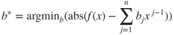
If our function is ![]() and we want a polynomial in degree
and we want a polynomial in degree ![]() , this gives the problem of finding the coefficients of the vector
, this gives the problem of finding the coefficients of the vector ![]() in
in
for all ![]() in some interval
in some interval ![]() .
.
Note that the goal is to approximate a function with a polynomial of given degree, and this is where the Remez approach is the one to use.
There is a discretized version of this problem where we attempt to find the solution over a discrete set of values of ![]() . Here is an example problem suggested by Hans Werner Borchers (Figure 14.1). Let us first get the least squares fit, which will provide some idea of where the solution may lie.
. Here is an example problem suggested by Hans Werner Borchers (Figure 14.1). Let us first get the least squares fit, which will provide some idea of where the solution may lie.
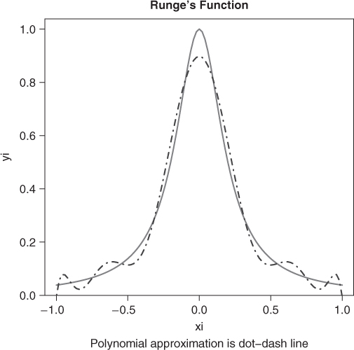
n <- 10  # polynomial of degree 10
m <- 101  # no. of data points
xi <- seq(-1, 1, length = m)
yi <- 1/(1 + (5 * xi)^2)
plot(xi, yi, type = "l", lwd = 3, col = "gray", main = "Runge's function")
title(sub = "Polynomial approximation is dot-dash line")
pfn <- function(p) max(abs(polyval(c(p), xi) - yi))
require(pracma)
pf <- polyfit(xi, yi, n)
print(pfn(pf))
## [1] 0.102366
lines(xi, polyval(pf, xi), col = "blue", lty = 4)
From the graph, the solution is clearly not a terribly good approximation, but may nonetheless serve us if we know the maximum absolute error over the 101 points in the interval ![]() .
.
## set up a matrix for the polynomial data
ndeg <- 10
Ar <- matrix(NA, nrow = 101, ncol = ndeg + 1)
Ar[, ndeg + 1] <- 1
for (j in 1:ndeg) {
    # align to match polyval
    Ar[, ndeg + 1 - j] <- xi * Ar[, ndeg + 2 - j]
}
cat("Check minimax function value for least squares fit
")
## Check minimax function value for least squares fit
print(minmaxw(pf, Ar, yi))
## [1] 0.102366
## attr(,"where")
## [1] 51
apoly1 <- mmreg(Ar, yi)
apoly1$mad
## [1] 0.0654678
pcoef <- apoly1$coeffs
pcoef
##           1           2           3           4           5
##  −50.248256    0.000000  135.853517    0.000000 −134.201071
##           6           7           8           9          10
##    0.000000   59.193155    0.000000  −11.558883    0.000000
##          11
##    0.934532
sumabs(pcoef, Ar, yi)
## [1] 4.28865
sumsqr(pcoef, Ar, yi)
## [1] 0.224028
print(minmaxw(pcoef, Ar, yi))
## [1] 0.0654678
## attr(,"where")
## [1]  3 99
## LAD regression on Runge
apoly2 <- LADreg(Ar, yi)
apoly2$sad
## [1] 3.06181
pcoef2 <- apoly2$coeffs
pcoef2
##            1            2            3            4
## −2.19324e+01  0.00000e+00  6.29108e+01  0.00000e+00
##            5            6            7            8
## −6.78485e+01  0.00000e+00  3.41440e+01 −1.39697e-12
##            9           10           11
## −8.11899e+00  4.66635e-14  8.45327e-01
sumabs(pcoef2, Ar, yi)
## [1] 3.06181
sumsqr(pcoef2, Ar, yi)
## [1] 0.211185
print(minmaxw(pcoef2, Ar, yi))
## [1] 0.154673
## attr(,"where")
## [1] 51
We can check the solution if we have a usable global minimization tool. It turns out that the usual stochastic tools (see Chapter 15) do rather poorly on this problem, but package adagio does find the same solution, albeit slowly.
require(adagio)
system.time(aadag <- pureCMAES(pf, pfn, rep(-200, 11), rep(200,
    11)))
##    user  system elapsed
##  32.110   1.684  33.815
aadag
## $xmin
##  [1] −5.02483e+01 −7.66372e-14  1.35854e+02  1.49894e-14
##  [5] −1.34201e+02 −5.40655e-14  5.91932e+01  1.07589e-13
##  [9] −1.15589e+01 −1.04359e-14  9.34532e-01
##
## $fmin
## [1] 0.0654678
References
- Berkelaar M et al. 2013 lpSolve: interface to Lp_solve v. 5.5 to solve linear / integer programs. R package version 5.6.7.
- Bhat KA 2011 Some aspects of mathematical programming in statistics PhD thesis Post Graduate, PhD Dissertation, Department of Statistics, University of Kashmir Srinagar, India.
- Bisschop J and Roelofs M 2006 AIMMS Optimization Modeling. Paragon Decision Technology in Haarlem, The Netherlands.
- Ghalanos A and Theussl S 2012 Rsolnp: General Non-linear Optimization Using Augmented Lagrange Multiplier Method. R package version 1.14.
- Harter R, Hornik K and Theussl S 2013 Rsymphony: Symphony in R. R package version 0.1-16.
- Henningsen A 2012 linprog: Linear Programming / Optimization. R package version 0.9-2.
- Hornik K, Meyer D and Theussl S 2011 ROI: R Optimization Infrastructure. R package version 0.0-7.
- Karatzoglou A, Smola A, Hornik K, and Zeileis A 2004 kernlab—an S4 package for kernel methods in R. Journal of Statistical Software 11(9), 1–20.
- Koenker R 2005 Quantile Regression. Cambridge University Press, Cambridge.
- Koenker R 2013 quantreg: Quantile Regression. R package version 5.05.
- McCarthy WF and Bateman DV 1988 The use of mathematical programming for designing dual frame surveys. Proceedings of the Survey Research Methods Section, 1988, pp. 652–653. American Statistical Association, Alexandria, VA.
- Pachón R and Trefethen LN 2009 Barycentric-Remez algorithms for best polynomial approximation in the chebfun system. BIT Numerical Mathematics 49(4), 721–741.
- Theussl S and Hornik K 2013 Rglpk: R/GNU Linear Programming Kit Interface. R package version 0.5-1.
- Turlach BA R port by Andreas Weingessel S 2013 quadprog: Functions to solve Quadratic Programming Problems. R package version 1.5-5.
- Varadhan R 2012 alabama: Constrained nonlinear optimization. R package version 2011.9-1.