
Chapter 16
Scaling and reparameterization
Both scaling—substituting scalar multiples of optimization parameters for those in the original model—and reparameterization—substituting invertible functions of optimization parameters for the parameters themselves—are tools that sometimes assist us to get solutions or else to reduce the computational effort to get solutions. Of course, scaling is but a simple form of reparameterization.
In this chapter, we will look at this topic. Unfortunately, while scaling and reparameterization are often recommended and are mathematically relatively simple, they are not trivial to use because they need to be applied carefully and, as with many topics in nonlinear optimization, the results may both help and impede the process of obtaining good results.
16.1 Why scale or reparameterize?
The essence of nonlinearity of a function ![]() is that the value of
is that the value of ![]() cannot be expressed in terms where the parameters appear to power 1. This can be important when we want to understand the functional surface of
cannot be expressed in terms where the parameters appear to power 1. This can be important when we want to understand the functional surface of ![]() . In some regions, a standard change—either absolute or percentage—in one of the parameters x will result in a small change in the value of
. In some regions, a standard change—either absolute or percentage—in one of the parameters x will result in a small change in the value of ![]() while in others the change will be very large.
while in others the change will be very large.
From the perspective of optimization, it is helpful to think of the optimization problem as akin to locating the bottom of a bowl. When we can visualize the whole object, this is easy, especially when ![]() is of dimension 2, and where these objects have a size where the width and height are of the same general order of magnitude. When, however, the bowl is 2 mm wide in one direction, 100 m front to back, and a 100 km high, we are dealing with a more difficult task. Similarly, high dimensionality strains our ability to imagine the surface.
is of dimension 2, and where these objects have a size where the width and height are of the same general order of magnitude. When, however, the bowl is 2 mm wide in one direction, 100 m front to back, and a 100 km high, we are dealing with a more difficult task. Similarly, high dimensionality strains our ability to imagine the surface.
Thus our first rationale for scaling is that we want to have the sizes of the parameters x more or less the same magnitude or expressed in units familiar to workers in a field of activity. I find a helpful rule of thumb is that all ![]() for
for ![]() in 1 :
in 1 : ![]() , where
, where ![]() is the number of parameters, should be between 1 and 10. Function minimization methods try to alter the parameters of
is the number of parameters, should be between 1 and 10. Function minimization methods try to alter the parameters of ![]() to make the function of the altered parameters
to make the function of the altered parameters ![]() smaller than that for the current set
smaller than that for the current set ![]() . Humans find it a great deal easier to envisage changes in the parameters when the parameters and the changes have similar sizes and scales. It may be helpful to think of the parameter sizes as being set on dials like the controls of a stove with settings from 1 to 10. It is very awkward to work with a stove if one burner goes from cold to red hot between 5.01 and 5.03, while another burner has 1.0–9.9 for the same range of heat.
. Humans find it a great deal easier to envisage changes in the parameters when the parameters and the changes have similar sizes and scales. It may be helpful to think of the parameter sizes as being set on dials like the controls of a stove with settings from 1 to 10. It is very awkward to work with a stove if one burner goes from cold to red hot between 5.01 and 5.03, while another burner has 1.0–9.9 for the same range of heat.
Worse, there may be regions where it makes no sense to seek an optimum. If the function ![]() is rapidly oscillating with small changes in one or more of the
is rapidly oscillating with small changes in one or more of the ![]() , it will be difficult for optimization tools that assume we are “finding the bottom of a bowl” to do their job. Regions where the function is discontinuous or even has discontinuous derivatives can also be problematic. For this discussion, we will set aside these worries, except as they illustrate scaling concerns.
, it will be difficult for optimization tools that assume we are “finding the bottom of a bowl” to do their job. Regions where the function is discontinuous or even has discontinuous derivatives can also be problematic. For this discussion, we will set aside these worries, except as they illustrate scaling concerns.
A second rationale is mainly a human issue in managing data and results. In recording or entering data, it is useful to not have to carry too many digits or to have to enter exponents, especially for values of parameters that are “close” to the optimum. For example, in the Hobbs weed infestation problem discussed in the following text, the scaled solution is “near” to the parameter values 2, 5, and 3, which are easily remembered and entered. Moreover, the display of a large number of digits, most of which may have no meaning in the context of the problem at hand, may lead users to believe the results of an estimation procedure are “accurate.” The potential for human error increases with the amount of information to be read or copied.
Arguments like this are clearly not sufficient to mandate scaling. Indeed, not all methods need the user to scale the function. However, scaling can be helpful, as we shall try to show by following examples.
A particular issue concerns parameters that are zero at the optimum. For some problems, such zero parameters may not be truly “there.” That is, the parameter may not be needed in a model that we are trying to estimate and could be dropped from the function. If the parameter really is part of our objective function, then we may see the scale of the parameter change rapidly relative to other parameters as methods progressively reduce the magnitude of the parameter in an attempt to optimize the objective function.
It is also possible to scale the objective function. I recommend doing this only to make the numbers sensible in the context of the problem or the field of application. Unfortunately, the function optim() has a feature for allowing a function scaling to be applied, but its usage example is to change the sign on the function so that the minimizers in optim() can maximize a function. My strong preference is to avoid calling this change of sign a “scaling,” especially as maximization appears to be the major, perhaps only, use of the feature.
16.2 Formalities of scaling and reparameterization
Scaling is part of the overall issue of reparameterization. For example, if there is an invertible set of functions z() (we use bold face to indicate that we are using a vector of functions here, one per parameter), we can write
A simple case uses a matrix transformation, for which we use a matrix we will call ![]() for convenience. Thus
for convenience. Thus
While ![]() can be any nonsingular matrix, a simple diagonal matrix with no zero entries on the diagonal provides us with what we often refer to as “scaling,” because we then just multiply each element of
can be any nonsingular matrix, a simple diagonal matrix with no zero entries on the diagonal provides us with what we often refer to as “scaling,” because we then just multiply each element of ![]() by the corresponding diagonal element of
by the corresponding diagonal element of ![]() to get the appropriate element of
to get the appropriate element of ![]() . We reverse the transformation by dividing the elements of
. We reverse the transformation by dividing the elements of ![]() by the diagonal elements of
by the diagonal elements of ![]() .
.
A similarly simple affine transformation uses offsets ![]() , so that the
, so that the ![]() th reparametrizing function is
th reparametrizing function is
This is a particular and simple case of an affine transformation between the raw and “scaled” parameters. The so-called “standardized” variables form such transformations using the population means for the shifts and population standard deviations for the scaling. Indeed, base R has a function scale() for just this purpose. For most purposes, because such population values are generally unknown, we are better off to use simpler numbers such aspowers of 10.
16.3 Hobbs' weed infestation example
We again use the Hobbs problem (Section 1.2).
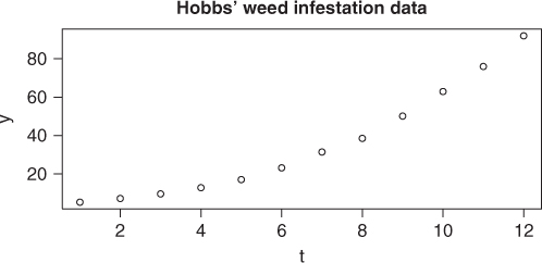
# draw the data
y <- c(5.308, 7.24, 9.638, 12.866, 17.069, 23.192, 31.443, 38.558, 50.156,
    62.948, 75.995, 91.972)
t <- 1:12
plot(t, y)
title(main = "Hobbs' weed infestation data", font.main = 4)
The problem was supplied by Mr Dave Hobbs of Agriculture Canada (Figure 16.1). As told to the author, the observations (![]() ) are weed densities per unit area over 12 growing periods. We were never given the actual units of the observations, without which I would now refuse to consider the problem. It was suggested that the appropriate model was a three-parameter logistic, that is,
) are weed densities per unit area over 12 growing periods. We were never given the actual units of the observations, without which I would now refuse to consider the problem. It was suggested that the appropriate model was a three-parameter logistic, that is,
where ![]() is the growing period.
is the growing period.
Now we will express the sum-of-squares function in R. First we will use an unscaled version of the loss function and residual. Then we will scale by simple powers of 10. Note that the data is embedded in the function.
hobbs.f<- function(x){ # # Hobbs weeds problem -- function
    if (abs(12*x[3])> 50) { # check computability
       fbad<-.Machine$double.xmax
       return(fbad)
    }
    res<-hobbs.res(x)
    f<-sum(res*res)
}
hobbs.res<-function(x){ # Hobbs weeds problem -- residual
# This variant uses looping
    if(length(x) != 3) stop("hobbs.res -- parameter vector n!=3")
    y<-c(5.308, 7.24, 9.638, 12.866, 17.069, 23.192, 31.443,
         38.558, 50.156, 62.948, 75.995, 91.972)
    t<-1:12
    if(abs(12*x[3])>50) {
       res<-rep(Inf,12)
    } else {
       res<-x[1]/(1+x[2]*exp(-x[3]*t)) - y
    }
}
Let us try running this problem in optim() using the standard Nelder–Mead method starting at the vector expressed as c(100, 10, 0.1). This unscaled start point corresponds to c(1, 1, 1) in the following scaled version.
cat("Running the Hobbs problem - code already loaded - with Nelder-Mead
")
## Running the Hobbs problem - code already loaded - with Nelder-Mead
start <- c(100, 10, 0.1)
f0 <- hobbs.f(start)
cat("initial function value=", f0, "
")
## initial function value= 10685.3
tu <- system.time(ansnm1 <- optim(start, hobbs.f, control = list(maxit = 5000)))[1]
# opt2vec is a small routine to convert answers to a vector form for
# printing
Unscaled1 <- opt2vec("unscaled Nelder", ansnm1)
## unscaled Nelder : f( 195.863 ,  49.0609 ,  0.313756 )= 2.58754
##     after  247  fn &  NA  gr evals
The following is a very simple scaling of the original problem. Here is the code for the function and residual.
shobbs.f<-function(x){ # # Scaled Hobbs weeds problem -- function
    if (abs(12*x[3]*0.1)> 50) { # check computability
       fbad<-.Machine$double.xmax
       return(fbad)
    }
    res<-shobbs.res(x)
    f<-sum(res*res)
}
shobbs.res<-function(x){ # scaled Hobbs weeds problem -- residual
# This variant uses looping
    if(length(x) != 3) stop("hobbs.res -- parameter vector n!=3")
    y<-c(5.308, 7.24, 9.638, 12.866, 17.069, 23.192, 31.443, 38.558, 50.156,
          62.948, 75.995, 91.972)
    t<-1:12
    res<-100.0*x[1]/(1+x[2]*10.*exp(-0.1*x[3]*t)) - y
}
Let us also try running the scaled version of the problem in optim using the standard Nelder–Mead method starting at the vector expressed as c(1, 1, 1).
cat("Running the scaled Hobbs problem - code already loaded - with Nelder-Mead
")
## Running the scaled Hobbs problem - code already loaded - with Nelder-Mead
start <- c(1, 1, 1)
f0 <- shobbs.f(start)
cat("initial function value=", f0, "
")
## initial function value= 10685.3
ts <- system.time(ansnms1 <- optim(start, shobbs.f, control = list(maxit = 5000)))[1]
opt2vec("scaled Nelder", ansnms1)
## scaled Nelder : f( 1.9645 ,  4.9116 ,  3.13398 )= 2.58765
##     after  196  fn &  NA  gr evals
The examples hint that the scaled version is slightly less work for the Nelder–Mead method to solve but that the advantage is not huge. We may hypothesize
- that scaled problems may have less difficulty finding a solution from a “random” or simple starting point.
- that from equivalent starting points, the scaled function may allow a solution to be found more efficiently, that is, with fewer function evaluations.
Let us apply a different optimizer (BFGS) to the same two tasks.
cat("Running the Hobbs problem - code already loaded - with BFGS
")
## Running the Hobbs problem - code already loaded - with BFGS
start <- c(100, 10, 0.1)
starts <- c(1, 1, 1)
f0 <- hobbs.f(start)
f0s <- shobbs.f(starts)
cat("initial function values: unscaled=", f0, "  scaled=", f0s, "
")
## initial function values: unscaled= 10685.3   scaled= 10685.3
tu <- system.time(abfgs1 <- optim(start, hobbs.f, method = "BFGS", control = list(maxit = 5000)))[1]
opt2vec("BFGS unscaled", abfgs1)
## BFGS unscaled : f( 196.194 ,  49.0884 ,  0.313556 )= 2.58728
##     after  209  fn &  59  gr evals
ts <- system.time(abfgs1s <- optim(starts, shobbs.f, method = "BFGS", control = list(maxit = 5000)))[1]
opt2vec("BFGS scaled", abfgs1s)
## BFGS scaled : f( 1.9619 ,  4.90919 ,  3.13568 )= 2.58728
##     after  118  fn &  36  gr evals
Here we see that scaling reduces the function/gradient count and gets a slightly lower final function value. Of course, we really should use analytic rather than numerically approximated gradients in the BFGS (actually variable metric) method. Let us put them in and run the same problems again.
hobbs.jac <- function(x) {
    # Jacobian of Hobbs weeds problem
    jj <- matrix(0, 12, 3)
    t <- 1:12
    yy <- exp(-x[3] * t)
    zz <- 1/(1 + x[2] * yy)
    jj[t, 1] <- zz
    jj[t, 2] <- -x[1] * zz * zz * yy
    jj[t, 3] <- x[1] * zz * zz * yy * x[2] * t
    return(jj)
}
hobbs.g <- function(x) {
    # gradient of Hobbs weeds problem NOT EFFICIENT TO CALL AGAIN
    jj <- hobbs.jac(x)
    res <- hobbs.res(x)
    gg <- as.vector(2 * t(jj) %*% res)
    return(gg)
}
shobbs.jac <- function(x) {
    # scaled Hobbs weeds problem -- Jacobian
    jj <- matrix(0, 12, 3)
    t <- 1:12
    yy <- exp(-0.1 * x[3] * t)
    zz <- 100/(1 + 10 * x[2] * yy)
    jj[t, 1] <- zz
    jj[t, 2] <- -0.1 * x[1] * zz * zz * yy
    jj[t, 3] <- 0.01 * x[1] * zz * zz * yy * x[2] * t
    return(jj)
}
shobbs.g <- function(x) {
    # scaled Hobbs weeds problem -- gradient
    shj <- shobbs.jac(x)
    shres <- shobbs.res(x)
    shg <- as.vector(2 * (shres %*% shj))
    return(shg)
}
cat("Running the Hobbs problem - code already loaded - with BFGS
")
## Running the Hobbs problem - code already loaded - with BFGS
start <- c(100, 10, 0.1)
starts <- c(1, 1, 1)
f0 <- hobbs.f(start)
f0s <- shobbs.f(starts)
cat("initial function values: unscaled=", f0, "  scaled=", f0s, "
")
## initial function values: unscaled= 10685.3   scaled= 10685.3
tu <- system.time(abfgs1g <- optim(start, hobbs.f, gr = hobbs.g, method = "BFGS", control = list(maxit = 5000)))[1]
opt2vec("BFGS unscaled", abfgs1g)
## BFGS unscaled : f( 196.175 ,  49.0885 ,  0.313573 )= 2.58728
##     after  127  fn &  50  gr evals
ts <- system.time(abfgs1sg <- optim(starts, shobbs.f, gr = shobbs.g, method = "BFGS", control = list(maxit = 5000)))[1]
opt2vec("BFGS scaled", abfgs1sg)
## BFGS scaled : f( 1.96186 ,  4.90916 ,  3.1357 )= 2.58728
##     after  119  fn &  36  gr evals
Here we see that we do not gain very much in terms of function/gradient counts by using the analytic gradients for the scaled function, but we do get better results for the unscaled problem, both in terms of function/gradient counts and also a lower final function value. This is likely due to the more or less fixed value used for the “eps” in computing a forward finite-difference approximation to the gradient (Section 10.5). While we actually could alter the shift for each dimension, as the documentation tells us, I do not believe that I have ever done this in R and do not expect users to be able to do so easily.
     'ndeps' A vector of step sizes for the finite-difference
          approximation to the gradient, on 'par/parscale' scale.
          Defaults to '1e-3'.
Let us try using the parscale offered by optim. Note that many optimization tools do NOT include this facility. For the BFGS method, we will include a trace so that we can check if the initial function value is as expected. It is easy to get the wrong scaling values in parscale.
cat("Try using parscale
")
## Try using parscale
start <- c(100, 10, 0.1)
anmps1 <- optim(start, hobbs.f, control = list(trace = FALSE, parscale = c(100,  10, 0.1)))
opt2vec("Nelder + parscale", anmps1)
## Nelder + parscale : f( 196.45 ,  49.116 ,  0.313398 )= 2.58765
##     after  196  fn &  NA  gr evals
abfps1 <- optim(start, hobbs.f, gr = hobbs.g, method = "BFGS", control = list(trace = TRUE, parscale = c(100, 10, 0.1)))
## initial  value 10685.287754
## iter  10 value 1023.938721
## iter  20 value 45.644964
## iter  30 value 2.629944
## final  value 2.587277
## converged
opt2vec("BFGS + parscale", abfps1)
## BFGS + parscale : f( 196.186 ,  49.0916 ,  0.31357 )= 2.58728
##     after  119  fn &  36  gr evals
Using parscale is, as we see, equivalent within some small rounding errors of using the explicit scaling. Possibly it is my own prejudice, but I prefer the explicit scaling and find it easier to use.
16.4 The KKT conditions and scaling
For an unconstrained objective function ![]() , the KKT (Karush–Kuhn–Tucker) conditions (Karush, 1939; Kuhn and Tucker, 1951) for a (local) minimum at y are that the gradient of
, the KKT (Karush–Kuhn–Tucker) conditions (Karush, 1939; Kuhn and Tucker, 1951) for a (local) minimum at y are that the gradient of ![]() at y is null and that the eigenvalues of the Hessian of
at y is null and that the eigenvalues of the Hessian of ![]() at y are all positive. The gradient is the vector of first derivatives of
at y are all positive. The gradient is the vector of first derivatives of ![]() with respect to the parameters (evaluated at
with respect to the parameters (evaluated at ![]() ). The Hessian is the matrix of second derivatives.
). The Hessian is the matrix of second derivatives.
Of course, “null” and “positive” are ideas that presume exact arithmetic. The reality is that we want the gradient to be “small.” For the Hessian, we want all eigenvalues positive as a first condition. That is relatively easy to check. However, if the ratio of smallest to largest eigenvalue is less than, say, 1e![]() , we may suspect that the Hessian is very close to singular. This means that we cannot be sure that we are at a local minimum. Interpreted another way, it suggests that it is difficult to determine the minimum as a region of parameter space may be “flat.”
, we may suspect that the Hessian is very close to singular. This means that we cannot be sure that we are at a local minimum. Interpreted another way, it suggests that it is difficult to determine the minimum as a region of parameter space may be “flat.”
Let us run these checks on the BFGS answer from the scaled Hobbs function using the analytic gradient. The function kktc() contains output (in the experimental version used here), so we will avoid duplication of output and not print the result kbfgs1sg.
## Loading required package: numDeriv
## results from KKT check of abfgs1sg solution (scaled, with gradient from BFGS)
## KKT test tolerances: for g =  0.0012207    for H =  0.012207
## Parameters: [1] 1.96186 4.90916 3.13570
## Successful convergence!
## Compute gradient approximation at finish
## Gradient:[1]  0.001991813 -0.000485584  0.002579320
## kkt1 =  TRUE
## Compute Hessian approximation
##          [,1]      [,2]     [,3]
## [1,] 12654.61 -3256.125 16021.06
## [2,] -3256.13   862.709 -4095.21
## [3,] 16021.06 -4095.206 20434.34
## Eigenvalues found
## [1] 33860.5130    76.3199    14.8306
## negeig =  FALSE
## evratio = 0.00043799
## kkt2 =  FALSE
The result is apparently “not so good.” However, if we try the same exercise with the latest parscale version of the unscaled Hobbs function abfps1 and the unscaled function with gradient (abfgs1g), we get the following output.
## results from KKT check of abfps1 solution (parscaled, with gradient from BFGS)
## KKT test tolerances: for g =  0.0012207    for H =  0.012207
## Parameters: [1] 196.18627  49.09165   0.31357
## Successful convergence!
## Compute gradient approximation at finish
## Gradient:[1]  1.99186e-05 -4.85596e-05  2.57938e-02
## kkt1 =  FALSE
## Compute Hessian approximation
##            [,1]        [,2]       [,3]
## [1,]    1.26546    -3.25613    1602.11
## [2,]   -3.25613     8.62709   -4095.21
## [3,] 1602.10555 -4095.20623 2043434.30
## Eigenvalues found
## [1] 2.04344e+06 4.24926e-01 4.41380e-03
## negeig =  FALSE
## evratio = 2.15998e-09
## kkt2 =  FALSE
## results from KKT check of abfgs1g solution (unscaled, with gradient from BFGS)
## KKT test tolerances: for g =  0.0012207    for H =  0.012207
## Parameters: [1] 196.174504  49.088545   0.313573
## Successful convergence!
## Compute gradient approximation at finish
## Gradient:[1]  3.03187e-05 -7.66194e-04  1.14352e-04
## kkt1 =  TRUE
## Compute Hessian approximation
##            [,1]        [,2]       [,3]
## [1,]    1.26561    -3.25643    1602.15
## [2,]   -3.25643     8.62775   -4095.21
## [3,] 1602.14587 -4095.21284 2043294.41
## Eigenvalues found
## [1] 2.04330e+06 4.24989e-01 4.41682e-03
## negeig =  FALSE
## evratio = 2.16161e-09
## kkt2 =  FALSE
Thus the unscaled functions apparently have better (i.e., smaller) gradients but the Hessian approximations are very close to being effectively singular. This latter feature of the Hobbs problem can cause difficulty for Newton-like methods.
Question: Is the poorer gradient always the case?
Answer: Not necessarily. The following is a very simple two-parameter function, which becomes “badly” scaled as skew gets larger. The solution is at parameter vector (0, 2).
diagfn <- function(par, skew = 1) {
    x <- par[1] * skew
    y <- par[2]
    a <- x + y - 2
    b <- x - y + 2
    fval <- a * a + 4 * b * b
}
diaggr <- function(par, skew = 1) {
    x <- par[1] * skew
    y <- par[2]
    a <- x + y - 2
    b <- x - y + 2
    g1 <- (2 * a + 8 * b) * skew
    g2 <- 2 * a - 8 * b
    gr <- c(g1, g2)
    return(gr)
}
## Diagonal function test
## Nelder-Mead results
##      skew        fmin         par1 par2  nf ng ccode
## an1     1 4.70738e-15 -2.06620e-08    2 105 NA     0
## an1g   10 2.27900e-13  1.57277e-08    2 109 NA     0
## an10  100 4.58041e-12 -5.02533e-09    2 103 NA     0
## gradient an1:
## [1]  2.28659e-08 -2.58505e-07
## gradient an10:
## [1] -1.44379e-06  2.57408e-06
## gradient an100:
## [1] -3.4527e-06  5.7009e-06
##
##  BFGS results
##         skew        fmin         par1 par2 nf ng ccode
## abf1       1 1.77099e-27 -2.21587e-14    2 10  3     0
## abf1g      1 2.83990e-29 -2.84217e-16    2  7  3     0
## abf10     10 1.01635e-19  9.89887e-12    2 26 11     0
## abf10g    10 1.01635e-19  9.89886e-12    2 26 11     0
## abf100   100 3.14335e-25 -1.22168e-15    2 39 10     0
## abf100g  100 3.14640e-25 -1.21920e-15    2 39 10     0
## gradient abf1:
## [1] -1.04805e-13 -6.21725e-14
## gradient abf1g:
## [1] -7.10543e-15  7.10543e-15
## gradient abf10:
## [1] -9.68713e-10  1.72011e-09
## gradient abf10g:
## [1] -9.68713e-10  1.72011e-09
## gradient abf100:
## [1]  1.56142e-12 -2.61657e-12
## gradient abf100g:
## [1]  1.56364e-12 -2.61791e-12
If we graph the function for different skew levels, we can see the problem. Here we just show the case for skew=10 (Figure 16.2). Increasing the skew parameter causes the function surface to look less like a bowl and more like a gutter. This is reflected in the differing curvatures in the two dimensions that can also be shown by the eigenvalues of the Hessian at the supposed minimum. However, the gradient size, while greater for the two larger values of skew, does not seem to follow a particular pattern, and what is seen may be rounding error.
x = seq(-15, 15, 0.5)
y = seq(-15, 15, 0.5)
## skew=1
nx <- length(x)
ny <- length(y)
z <- matrix(NA, nx, ny)
z10 <- z
z100 <- z
k <- 0
for (i in 1:nx) {
    for (j in 1:ny) {
        par <- c(x[i], y[j])
        val <- diagfn(par, skew = 1)
        val10 <- diagfn(par, skew = 10)
        val100 <- diagfn(par, skew = 100)
        z[i, j] <- val
        z10[i, j] <- val10
        z100[i, j] <- val100
    }
}
persp(x, y, z10, theta = 20, phi = 10, expand = 0.5, col = "lightblue", ltheta = 120, shade = 0.75, ticktype = "detailed", xlab = "X", ylab = "Y",
    zlab = "Z")
title("Diagonal function for skew = 10")

16.5 Reparameterization of the weeds problem
The three-parameter logistic model used above can take a somewhat different form, namely,
where ![]() is often renamed Asym. Clearly we can easily transform one form to the other, or to the scaled version
is often renamed Asym. Clearly we can easily transform one form to the other, or to the scaled version shobbs(). The form (16.7) is used in the SSlogis self-starting nonlinear model in R developed by Doug Bates. This form permits a useful geometric interpretation of the parameters in relation to the S-shape of the model. The first parameter, ![]() or Asym, is the upper asymptote of the curve; xmid is the
or Asym, is the upper asymptote of the curve; xmid is the ![]() -axis position of the point where the curve is half way from the lower to the upper asymptote; scal controls the rate at which the curve rises. Smaller values of scal result in curves that rise more steeply. This interpretation is helpful in selecting especially the first two parameters and in guiding the selection of the third. However, does it result in a higher chance of success with our optimizers? We address this after the next section.
-axis position of the point where the curve is half way from the lower to the upper asymptote; scal controls the rate at which the curve rises. Smaller values of scal result in curves that rise more steeply. This interpretation is helpful in selecting especially the first two parameters and in guiding the selection of the third. However, does it result in a higher chance of success with our optimizers? We address this after the next section.
16.6 Scale change across the parameter space
Nonlinear optimization is carried out in an Alice-in-Wonderland environment where the scale is different in different parts of the space. To see this more clearly, we can vary the parameters of the different Hobbs models by 1% at the start of the optimization and at its end. For convenience, we work with the scaled Hobbs function as our base model and use the starting parameter vector c(1,1,1). We transform this start for the unscaled Hobbs model and the Hobbs–Bates model. Moreover, we optimize only the scaled Hobbs function and then transform the parameters for the other two models at the supposed optimum. However, we do re-evaluate the unscaled and Bates functions to ensure we have the same solution.
##                   fn value 1% p1 effect 1% p2 effect 1% p3 effect
## shobbs - start 10685.28775    -0.941062     0.729787    -0.771187
## uhobbs - start 10685.28775    -0.941062     0.729787    -0.771187
## hbates - start 10685.28775    -0.941062     1.689136    -0.906786
## shobbs - final     2.58765    92.435940    40.769094   387.872740
## uhobbs - final     2.58765    92.435940    40.769094   387.872740
## hbates - final     2.58765    92.435940   605.478530    47.916044
The table shows that the effect of shifting one of the parameters by 1% near the starting parameters has a modest effect on the sum-of-squares function value. Indeed, the change in the function value is at most a modest 1.7%. By contrast, at the minimum, changing the asymptote parameter (![]() ,
, ![]() , or Asym) changes the sum of squares by better than 92%. For similar percentage changes to the other two parameters, both the
, or Asym) changes the sum of squares by better than 92%. For similar percentage changes to the other two parameters, both the hobbs.f() and shobbs.f() change identically, but for a 1% change in the parameters, the functions change roughly 41 and 388%, respectively. The Bates reparameterization is different, with the sum of squares being highly sensitive to the xmid parameter—a 605% change, while a 1% change in scal “only” results in a 48% change.
16.7 Robustness of methods to starting points
We are now in a position to examine whether scaling or reparameterization allows us to find solutions more easily. A frequent admonition to novice users of optimization and nonlinear modeling is to choose different and hopefully better starting points for the iterative methods. However, this is not always useful advice. If we knew our answer, we would not need the optimization!
For this exercise, we originally created 1000 points generated pseudo-randomly in a box that is bounded by 0 and 5 for each of the three scaled parameters. We then generated the unscaled and Bates starts. The code looked like this.
# generate 1000 sets of points in [0, 5) with runif()
set.seed(12345)
nrun <- 1000
sstart <- matrix(runif(3 * nrun, 0, 5), nrow = nrun, ncol = 3)
ustart <- sstart %*% diag(c(100, 10, 0.1))
bstart <- matrix(NA, nrow = nrun, ncol = 3)
for (i in 1:nrun) {
    b1 <- ustart[[i, 1]]
    b2 <- ustart[[i, 2]]
    b3 <- ustart[[i, 3]]
    Asym <- b1
    scal <- 1/b3
    xmid <- log(b2)/b3
    bstart[[i, 1]] <- Asym
    bstart[[i, 2]] <- xmid
    bstart[[i, 3]] <- scal
}
As the starts are equivalent, we can compare performance for the three models, namely, unscaled, scaled, and Bates. This exercise showed poorer results for the Bates model than I had expected, and in checking, I discovered that some starting parameter sets were inadmissible for the Bates model—infinite or NaN results were returned in function or gradient calculations. I then tried starting with the Bates model and generated points as in the code below. Note that we now restrict the Asym parameter to be larger than 92 (the largest data value). This is not an absolute requirement because data can be higher or lower than our model, but it does avoid some inadmissible starts. Furthermore, the xmid parameter is limited to be between 2 and 11, and scal bigger than 0.05.
## random Bates start generate 1000 sets of points in [0, 5) with runif()
set.seed(12345)
nrun <- 1000
bstart <- matrix(runif(3 * nrun, 0, 1), nrow = nrun, ncol = 3)
minasymp <- 92
bstart[, 1] <- bstart[, 1] * (500 - minasymp) + minasymp
bstart[, 2] <- bstart[, 2] * 9 + 2  # inside t interval
scal0 <- 0.05
bstart[, 3] <- bstart[, 3] * (5 - scal0) + scal0  # No check for zero!
sstart <- matrix(NA, nrow = nrun, ncol = 3)
ustart <- sstart
for (i in 1:nrun) {
    Asym <- bstart[[i, 1]]
    xmid <- bstart[[i, 2]]
    scal <- bstart[[i, 3]]
    b1 <- Asym
    b2 <- exp(xmid/scal)
    b3 <- 1/scal
    ustart[[i, 1]] <- b1
    sstart[[i, 1]] <- b1/100
    ustart[[i, 2]] <- b2
    sstart[[i, 2]] <- b2/10
    ustart[[i, 3]] <- b3
    sstart[[i, 3]] <- b3 * 10
}
dput(bstart, file = "supportdocs/scaling/batestrtb.dput")
dput(sstart, file = "supportdocs/scaling/batestrts.dput")
dput(ustart, file = "supportdocs/scaling/batestrtu.dput")
However, even with the precautions in generating parameters above for the Bates model, the models sometimes gave infinite or NaN results on initial evaluation when trying the optimizations. Thus we eliminated some points from the starting set by finding the unique set that caused failure for any of the three models.
exlist <- c()  # empty
extype <- c()  # to record type
nex = 0
cat("Run scaled model -- ")
## Run scaled model --
for (i in 1:nrun) {
    # for (i in 150:160) {
    st <- as.numeric(bstart[i, ])
    ga <- hbates.g(st)
    badgrad <- FALSE
    if (any(is.na(ga)) | any(!is.finite(ga)))
        badgrad <- TRUE
    if (badgrad) {
        exlist <- c(exlist, i)
        extype <- c(extype, "B")
    }
}
cat("found ", length(exlist) - nex, " bad starts
")
## found  0  bad starts
nex <- length(exlist)
cat("Run scaled model -- ")
## Run scaled model --
for (i in 1:nrun) {
    # for (i in 150:160) {
    st <- as.numeric(sstart[i, ])
    ga <- shobbs.g(st)
    badgrad <- FALSE
    if (any(is.na(ga)) | any(!is.finite(ga)))
        badgrad <- TRUE
    if (badgrad) {
        exlist <- c(exlist, i)
        extype <- c(extype, "S")
    }
}
cat("found ", length(exlist) - nex, " bad starts
")
## found  0  bad starts
nex <- length(exlist)
cat("Run unscaled model -- ")
## Run unscaled model --
for (i in 1:nrun) {
    # for (i in 150:160) {
    st <- as.numeric(ustart[i, ])
    ga <- hobbs.g(st)
    badgrad <- FALSE
    if (any(is.na(ga)) | any(!is.finite(ga)))
        badgrad <- TRUE
    if (badgrad) {
        exlist <- c(exlist, i)
        extype <- c(extype, "U")
    }
}
cat("found ", length(exlist) - nex, " bad starts
")
## found  38  bad starts
nex <- length(exlist)
exlist <- unique(exlist)
options(width = 80)
print(exlist)
##  [1]  11  38  94  99 119 120 175 265 281 347 358 373 442 446 474 538 541 551 557
## [20] 579 595 599 615 620 623 671 693 723 731 774 776 780 832 871 878 900 945 986
We can now proceed to discover how well different methods fare in optimizing the sum-of-squares function under the three models.
16.7.1 Robustness of optimization techniques
Using package optimx, the code for running the calculations is straightforward but tedious and will be omitted here.
## Loading required package: optimx
## Result has function value < 2.6
##
##           hbates shobbs uhobbs Total
##   ss>=2.6   6155   4860   8101 19116
##   ss <2.6   7187   8482   5241 20910
##   Total    13342  13342  13342 40026
These results indicate that despite the stabilization provided by the reparameterization, the Bates model gives a lower success rate than the scaled Hobbs model, with the unscaled model showing much lower success. If we restrict our measure of success to those results also satisfying the KKT conditions, the unscaled model fails miserably, although this is likely a direct result of the lack of scaling. This lack of scaling increases the condition number of the unscaled Hessian, but the tolerances used for the KKT tests in optimx are 0.001 for the gradient and 1e![]() for the ratio of the smallest to largest Hessian eigenvalues. Note that the solution we are working with is the application of
for the ratio of the smallest to largest Hessian eigenvalues. Note that the solution we are working with is the application of optim() method BFGS to the first random start of the unconstrained Hobbs model. We scale this solution and compute the scaled Hobbs model quantities. The application of BFGS to the scaled version of the same start in the scaled Hobbs model actually does not succeed in finding a good solution. Such is life with nonlinear modeling.
brunall$lt2.6k <- (brunall$lt2.6 & brunall$kkt1 & brunall$kkt2)
myopt26k <- table(brunall$lt2.6k, brunall$model, useNA = "no")
print(myopt26k)
##
##         hbates shobbs uhobbs
##   FALSE   7841   7355  13342
##   TRUE    5501   5987      0
## Get the first unscaled solution parameters
hobbu1 <- as.numeric(c(brunu[1, "b1"], brunu[1, "b2"], brunu[1, "b3"]))
cat("First unscaled solution has sum of squares=", hobbs.f(hobbu1), "
")
## First unscaled solution has sum of squares= 22.9947
require(numDeriv)
hessu1 <- hessian(hobbs.f, hobbu1)
## Hessian of the unscaled function at this solution
print(hessu1)
##            [,1]         [,2]        [,3]
## [1,]   0.225654    -0.998173     910.864
## [2,]  -0.998173     4.427138   -3989.510
## [3,] 910.863644 -3989.509799 3756349.376
## Eigenvalues
print(eigen(hessu1)$value)
## [1]  3.75635e+06  1.94973e-01 -1.96168e-04
## Gradient of unscaled function
print(as.numeric(hobbs.g(hobbu1)))
## [1]  0.0751719 -0.1095026 48.5989307
hobbu1s <- hobbu1 * c(0.01, 0.1, 10)  # scale the parameters
## Hessian of the scaled function at this solution (when scaled)
shessu1 <- hessian(shobbs.f, hobbu1s)
print(shessu1)
##          [,1]      [,2]     [,3]
## [1,] 2256.543  -998.173  9108.64
## [2,] -998.173   442.714 -3989.51
## [3,] 9108.636 -3989.510 37563.49
## Eigenvalues
print(eigen(shessu1)$value)
## [1] 40200.24451    63.07288    -0.56663
## Gradient of scaled function
print(as.numeric(shobbs.g(hobbu1s)))
## [1]  7.51719 -1.09503  4.85989
In the above tables, we are working with 14 methods on slightly fewer than 1000 starting points. We can segment the results by method. We only display the counts where the result is “good,” namely, the sum of squares is less than 2.6 and will ignore the KKT conditions.
##              hbates shobbs uhobbs   Sum
##
## BFGS            195    298    501   994
## bobyqa          925    842     79  1846
## CG                8      1      0     9
## hjkb            266    874     19  1159
## L-BFGS-B        944    833    373  2150
## Nelder-Mead     393    675    301  1369
## newuoa          950    848    183  1981
## nlm             186    256    181   623
## nlminb          946    897    861  2704
## nmkb            896    764    588  2248
## Rcgmin          329    358    627  1314
## Rvmmin          210    349    717  1276
## spg              16    754      0   770
## ucminf          923    733    811  2467
## Sum            7187   8482   5241 20910
Here we see that the scaled model has a decided advantage over the unscaled one. For some of the methods, the scaled model seems favored in comparison to the Bates reparameterization.
16.7.2 Robustness of nonlinear least squares methods
For nonlinear least squares solvers, we can perform a similar robustness exercise, using the same starting points to allow for comparisons. Here we will not follow through with the Hessian eigenvalues, but only look at results where the sum of squares does not exceed 2.6.
## Loading required package: nlmrt
## Loading required package: minpack.lm
## save computation by reading data
nlruns <- dget(file = "supportdocs/scaling/nlruns.dput")
nlrunu <- dget(file = "supportdocs/scaling/nlrunu.dput")
nlrunb <- dget(file = "supportdocs/scaling/nlrunb.dput")
nlrunall <- rbind(nlruns, nlrunu, nlrunb)
nlrunall <- as.data.frame(nlrunall)
nlrunall[, "meth"] <- as.character(nlrunall[, "meth"])
nlrunall[, "model"] <- as.character(nlrunall[, "model"])
nlrunall <- as.data.frame(nlrunall)
rownames(nlrunall) <- NULL
nlrunall$value[which(is.na(nlrunall$value))] <- 1e+300
nlrunall$lt2.6 <- FALSE
nlrunall$lt2.6[which(nlrunall$value < 2.6)] <- TRUE
## Successes by models and methods
mynltab <- table(nlrunall$lt2.6, nlrunall$meth, nlrunall$model)[2, , ]
mynltab <- addmargins(mynltab)
rownames(mynltab) <- c(rownames(mynltab)[1:3], "Total")
colnames(mynltab) <- c(colnames(mynltab)[1:3], "Total")
print(mynltab)
##
##         hbates shobbs uhobbs Total
##   nls      902    695    695  2292
##   nlsLM    962    816    817  2595
##   nlxb     960    879    919  2758
##   Total   2824   2390   2431  7645
In the above table, it is clear that the Bates form of the model is the easiest for the methods to solve from random starts. It also appears that nlxb() does a little better than nlsLM(). I believe (but have not verified) that this is due to the latter code using some elements of nls() and not attempting a solution when the Jacobian is effectively singular at the start. By contrast, I did not bother to check this possibility in writing nlxb(), and the Levenberg–Marquardt stabilization is able to move the parameters to values where the sum of squares is reduced. I have seen instances of this behavior on several occasions. nls() also seems to exit in a “failure” if a singular Jacobian is encountered along the minimization trajectory.
There are also some “failures” that I did investigate where the reported result is on a plateau or saddle point with small residual and/or near singular Hessian. One such is obtained by nlsLM() or nlxb() from starting point 67 when trying to use the scaled Hobbs model. Note that it is important to properly initiate the random number generator to be able to reproduce results in cases like this. That is, starting parameter set 67 is dependent on how we initiate the random number generator and how we subsequently generate parameter values.
We omit some of the exploratory work to find the particular solution to examine but give a few hints on how the search is done. Here we use the final parameters found by nlsLM() from this starting point with the scaled Hobbs model. Computing the gradient and the Hessian, we see that whether we use scaled or unscaled models, the Hessian is effectively singular, but the gradient is not null. nls() does not return a solution for this start and model, while nlxb() returns a result similar to that examined.
which(nlrunall$start == 67)
## [1]  193  194  195 3079 3080 3081 5965 5966 5967
test <- nlrunall[195, ]
print(test)
##          b1       b2      b3   value conv start  model  meth lt2.6
## 195 40.2016 -19420.6 1.80099 9133.98    0    67 shobbs nlsLM FALSE
tpar <- c(test["b1"], test["b2"], test["b3"])
tpar <- unlist(tpar)  # this seems to be necessary
spar <- tpar * c(0.01, 0.1, 10)  # scaled parameters
names(spar) <- snames
## scaled parameters
ftest <- shobbs.f(spar)
ftest
## [1] 9133.98
gg <- shobbs.g(spar)
gg
## [1]  0.510063  0.482318 70.795188
require(numDeriv)
## We use jacobian of gradient rather than hessian of function
hh <- jacobian(shobbs.g, spar)
hh
##              [,1]        [,2]        [,3]
## [1,] 188371.37634 -2.76132097 -5258.67826
## [2,]     -2.76132  0.00787602     8.03935
## [3,]  -5258.67826  8.03935276  8548.91821
eigen(hh)$values
## [1] 1.88525e+05 8.39527e+03 2.90094e-04
## ... BUT ...
utest <- hobbs.f(tpar)
utest
## [1] 9133.98
gu <- hobbs.g(tpar)
gu
## [1] 5.10063e-03 4.82318e-02 7.07952e+02
hu <- jacobian(hobbs.g, tpar)
eigen(hu)$values
## [1] 8.54892e+05 1.85137e+01 2.90094e-06
16.8 Strategies for scaling
From the above examples, let us distill some ideas on how to approach scaling in nonlinear models.
First, if your work is exploratory, and you work interactively, it is possible that you do not need to spend a lot of effort on scaling. In this case, my inclination is to try the computations in the form that is presented to you, but watch for obvious differences in scale. If it is easy to adjust the computations, as in the scaled Hobbs versus unscaled form, then that seems to be a worthwhile thing to do.
For scripts that are to be run by others and/or automated into tools where there will be limited chance for meaningful intervention, there is a much higher level of scrutiny needed. One then looks to arrange that parameters are in a reasonable scale and that all have a moderately similar magnitude. Starting values should be considered for their concordance with reality of the underlying system. We did this with the Hobbs problem by considering that the Asym parameter should not be less than the largest value of the modeled variable.
As I will state in other words elsewhere, highly accurate starting values are generally not needed, but really wild or lazy choices are asking for trouble. Generally, some quite simple rules can generate good starts. I recommend loose bounds on parameters to keep them away from ridiculous values.
Transformations are valuable but can be time consuming and error prone to code. However, for parameters that must be positive, I suggest using ![]() as the working parameter. Suppose we wanted the asymptote Asym to always be positive inside the model functions. Then
as the working parameter. Suppose we wanted the asymptote Asym to always be positive inside the model functions. Then ![]() would be chosen as the working parameter and early in the central function that computes the residuals (for a nonlinear least squares) we would have
would be chosen as the working parameter and early in the central function that computes the residuals (for a nonlinear least squares) we would have
Asym <- exp(Asyml)
Asym is now always positive, but we do not impose a bounds constraint separately.
After results are obtained, I believe it is almost always worth checking the KKT conditions. This can be computationally expensive but making use of erroneous values is much more directly costly to us in money, effort, and reputation. Of course, before running the KKT calculations, it is a really good idea to check that the optimizer used has returned a satisfactory termination code. I have on a number of occasions seen messages “Your program does not work right” from users who have not bothered to note that conv or some similarly named return code is telling them the results are likely wrong.
References
- Karush W 1939 Minima of functions of several variables with inequalities as side constraints. Master's thesis, MSc Dissertation, Department of Mathematics, University of Chicago, Chicago, IL.
- Kuhn HW and Tucker AW 1951 Nonlinear programming. Proceedings of 2nd Berkeley Symposium, pp. 481–492, Berkeley, USA.