
Chapter 11
Bounds constraints
Bounds, sometimes called box constraints, are among the most common constraints that users wish to impose on nonlinear optimization or modeling parameters. Fortunately, they are also quite easy to include, although as always care is needed in their implementation and use.
In this treatment, I will generally use the term “bounds.” In fact, we will not always impose a lower and upper bounds on every parameter, so we will not always have a “box,” and some methods do not lend themselves to imposing a true ![]() -dimensional box in which we will seek a solution.
-dimensional box in which we will seek a solution.
The general conditions we wish to satisfy are, therefore,
11.1 Single bound: use of a logarithmic transformation
Suppose we want one of our optimization parameters—call it ![]() —to be nonnegative in our modeling or objective function
—to be nonnegative in our modeling or objective function ![]() . For the moment, we will ignore other inputs to
. For the moment, we will ignore other inputs to ![]() , and we will leave the generalization to bounds other than zero until later. Clearly, we could rewrite our function to use a different parameter
, and we will leave the generalization to bounds other than zero until later. Clearly, we could rewrite our function to use a different parameter ![]() and then compute
and then compute ![]() or
or ![]() . The second form has, in my experience, worked a little better. It avoids the degeneracy that
. The second form has, in my experience, worked a little better. It avoids the degeneracy that ![]() and
and ![]() give the same value of
give the same value of ![]() , which may give some issues for different optimization tools.
, which may give some issues for different optimization tools.
We therefore have the transformation from our original parameter to the internal parameter over which we optimize as
and the reverse as
We need to ensure that we apply these transformations as appropriate, namely,
- At the call to the optimization or parameter determination routine, we need to transform the starting value of
 to the equivalent
  for each relevant parameter.
 - On each call to our objective function or its derivatives, the
 must be computed from
  . Note that this may be needed for each of several parameters.
 - On reporting or using the results, we need to generate the “solution” value of
 in the same way.
As an example, let us return to finding the minimum of the Lennard–Jones potential (Section 5.1),
# The L-J potential function
ljfne <- function(logr, ep = 0.6501696, sig = 0.3165555) {
    r <- exp(logr)
    fn <- 4 * ep * ((sig/r)^12 - (sig/r)^6)
}
# Use next line to see a graph of the transformed function
# curve(ljfne, from=log(0.3), to=log(1))
min <- optimize(ljfne, interval = c(-10, 10))
print(min)
## $minimum
## [1] -1.0347
##
## $objective
## [1] -0.65017
cat("In the original scale, minimum is at ", exp(min$minimum), "
")
## In the original scale, minimum is at  0.35532
We note that this answer corresponds to that found in Section 5.1, but we have not had to be so careful in specifying the interval in which a minimum is sought.
11.2 Interval bounds: Use of a hyperbolic transformation
A similar idea can be applied when we have open interval bounds, that is,
where we do not include the bound in the feasible set. Where all parameters are bounded, we have a “box,” but the surface of the box is outside the feasible domain. This is used in package dfoptim, Tim Kelley's variant of the Nelder–Mead polytope algorithm.
The idea is that the range of the hyperbolic tangent function tanh() is ![]() . Once again, let us call our parameter
. Once again, let us call our parameter ![]() and seek a new, internal, parameter
and seek a new, internal, parameter ![]() that is unconstrained while
that is unconstrained while ![]() can only take values in the interval [lower, upper]. This can be accomplished if
can only take values in the interval [lower, upper]. This can be accomplished if ![]() and
and ![]() are related by the expression
are related by the expression
To reverse the transformation, for example, to get starting parameter values, we use
Sometimes the tanh() function is too close to a step function or else too slowly changing. In these situations, we need to scale the new parameter ![]() by a number smaller or larger than 1, respectively. In the following example, we use 0.25 to “stretch” the variation of
by a number smaller or larger than 1, respectively. In the following example, we use 0.25 to “stretch” the variation of ![]() with
with ![]() .
.
11.2.1 Example of the tanh transformation
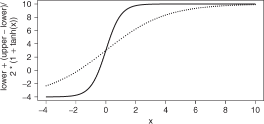
Let us impose the bounds
and look at the relationship of ![]() and
and ![]() . The solid line is the transformation above, while the dotted line uses
. The solid line is the transformation above, while the dotted line uses ![]() inside the expression (Figure 11.1).
inside the expression (Figure 11.1).
11.2.2 A fly in the ointment
The approach we have just presented is quite effective, and as we have indicated, it is used in the function nmkb() in package dfoptim. There is, however, one shortcoming, in that we cannot provide any initial parameter on a bound. Indeed, we must provide starting values strictly “inside the box.” While, in principle, this is not a great difficulty, it can be a nuisance and it needs to be kept in mind when using nmkb, especially inside wrappers such as optimx() where the returned “solutions” will have indicator values such as a very large number for the objective function. An alternative, which I prefer but demands quite a bit of extra programming work, is to check if starting parameters are on a bound.
As an example, consider the (contrived) function below, where we set the lower bounds at 2 for all parameters and the upper bounds at 4 and start at the lower bounds. Here we choose to use a four-parameter example, but the problem is of variable size. The correct solution has only the penultimate parameter free, that is, not on a bound, with the last parameter at the upper bound and the rest at the lower bound.
require(optimx)
flb <- function(x) {
    p <- length(x)
    sum(c(1, rep(4, p - 1)) * (x - c(1, x[-p])^2)^2)
}
start <- rep(2, 4)
lo <- rep(2, 4)
up <- rep(4, 4)
ans4a <- try(optimx(start, fn = flb, method = c("nmkb"), lower = lo,
    upper = up))
## Warning: nmkb() cannot be started if any parameter on a bound
11.3 Setting the objective large when bounds are violated
A rather old trick in optimization is to set the objective to a very large value whenever a constraint is violated. This will clearly disrupt gradient methods, because we are imposing discontinuities on the objective function. However, it is a technique that can be used for methods that purportedly do not use function values per se. The Hooke and Jeeves 1961 method and other pattern search techniques are of this type, but to my knowledge, only hjk() from dfoptim of this family is available for R at the time of writing. However, hjkb() from the same package already deals with bounds much more efficiently, because it works with axis search directions.
Some workers argue that the “large value” approach is suitable for use with the Nelder–Mead method, but I tend to agree with John Dennis that it is motivated by ideas of smooth functions, even though it does not explicitly require them. A simple example is illustrative.
flbp <- function(x, flo, fup) {
    p <- length(x)
    val <- sum(c(1, rep(4, p - 1)) * (x - c(1, x[-p])^2)^2)
    if (any(x < flo) || any(x > fup))
        val <- 1e+300
    val
}
start <- rep(2, 4)
lo <- rep(2, 4)
up <- rep(4, 4)
ans4p <- optimx(start, fn = flbp, method = c("hjkb", "Nelder-Mead",
    "nmkb"), flo = lo, fup = up)
## Warning: bounds can only be used with method L-BFGS-B (or Brent)
print(summary(ans4p))
##             p1     p2     p3     p4       value fevals
## hjkb         2 2.0000 2.1091 4.0000  3.2106e+01    332
## Nelder-Mead NA     NA     NA     NA 8.9885e+307     NA
## nmkb         2 2.0773 2.0000 3.6106  3.7836e+01    499
##             gevals niter convcode  kkt1  kkt2 xtimes
## hjkb            NA    19        0 FALSE FALSE  0.008
## Nelder-Mead     NA    NA     9999    NA    NA  0.004
## nmkb            NA    NA        0 FALSE FALSE  0.060
Despite the output, and the use of the name “hjkb” when in fact the unconstrained Hooke and Jeeves method is in use, this is the only method where the “large value” approach has found success. Given this example of a simple function, I do not recommend the approach.
11.4 An active set approach
The approach I have used to bounds in various packages I have put together involves an active set indicator to bounds constraints. The indicator vector maintains a record that tells whether a parameter is at a bound or not. We can use the same index to impose masks, that is, fixed parameters.
The particular choice of the set of values for the indicator can be important to make implementation easier. Also it is useful to have a consistent system for the indicator across different packages so code can be reused. The choices I have made are consistent with those used in the BASIC codes I developed with Mary Walker-Smith in 1987. These are as follows.
- Free parameters that are currently NOT at a bound have indicator 1.
- Fixed (masked) parameters are assigned an indicator 0.
- Parameters at an upper bound have indicator
 .
. - Parameters at an lower bound have indicator
 .
.
The choice of ![]() and
and ![]() was chosen so adding 2 to the indicator gives either a 1 or
was chosen so adding 2 to the indicator gives either a 1 or ![]() value that can be used in a simple multiplication with the gradient to decide if the objective is increasing or decreasing in the direction of the bound. This is useful in determining the gradient projection during the development of a search direction. Again for historical reasons, I call the indicator
value that can be used in a simple multiplication with the gradient to decide if the objective is increasing or decreasing in the direction of the bound. This is useful in determining the gradient projection during the development of a search direction. Again for historical reasons, I call the indicator bdmsk.
The main steps in using this approach repeat for each iteration of a method.
- At the start of the iteration, the gradient (or a proxy) is computed. For each component
 of the gradient, if
 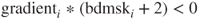 , then the objective DECREASES as we hit the bound, so we cannot proceed in that direction without moving into the infeasible region. In this case, we set
  . Otherwise, we “free” the parameter by setting
  .
. - Once we have a search direction
 , we want to perform a line search along it. However, we cannot proceed further than the upper or lower bound in each parameter direction. If the current parameters are par, then for
  , we can only go as far as
  , while if
  , the limit is
  . Clearly, if
  , we need not limit the stepsize. Looping over all components of
  , we reduce the steplength allowed for the line search to the smallest value found.
 - Once our line search selects a steplength and new set of parameters, we check the bounds and reset indicators appropriately. Clearly, we only need to look at currently free parameters. However, there is the consideration that we may have move to a point very close to a bound. This forces us to use a tolerance for the “closeness.” I check if
11.8

with a similar test on upper bounds. This test is scaled to the size of the bound, with 1 added to avoid difficulties with the very commonly encountered bound at zero. For ceps, I have been using
 macheps, where macheps is the floating-point machine precision in use. However, I am always concerned that tolerances such as this will be inappropriate for some problems.
Rvmmin() from the package of the same name uses this approach. I believe, but have not closely examined the codes, that method L-BFGS-B from the function optim() and bobyqa() from package minqa use similar techniques.
ans4 <- optimx(start, fn = flb, method = c("Rvmmin", "L-BFGS-B",
    "bobyqa"), lower = lo, upper = up, control = list(usenumDeriv = TRUE))
## Warning: Replacing NULL gr with 'numDeriv' approximation
print(summary(ans4))
##          p1 p2     p3 p4  value fevals gevals niter
## Rvmmin    2  2 2.1091  4 32.106    106     22    NA
## L-BFGS-B  2  2 2.1091  4 32.106      7      7    NA
## bobyqa    2  2 2.1091  4 32.106     44     NA    NA
##          convcode  kkt1 kkt2 xtimes
## Rvmmin          0 FALSE TRUE  0.012
## L-BFGS-B        0 FALSE TRUE  0.004
## bobyqa          0 FALSE TRUE  0.000
11.5 Checking bounds
Setting bounds, as we shall discuss in the following text, can assist in getting appropriate solutions to optimization and nonlinear equations problems. However, there is no guarantee that software will respect these bounds. It is, therefore, especially important to check that starting values of parameters are consistent with these bounds.
I regard starting values as infeasible if they are violate constraints. Some authors, quite reasonably, choose to reset starting values to the nearest bound that makes the starting values feasible. (This will not work for programs such as nmkb that use the transfinite function approach to bounds.)
It is also sensible to check solutions AFTER optimization to ensure that the constraints are still satisfied. I have seen several cases where optimization codes failed to respect constraints, even though that was a stated capability. I have also seen bounds-constrained optimizations that simply failed to achieve the true bounded optimum.
require(optextras)
## extract first solution from ans4
ans41 <- ans4[1, ]
c41 <- coef(ans41)  ## get coefficients
bdc <- bmchk(c41, lower = lo, upper = up, trace = 1)
## admissible =  TRUE
## maskadded =  FALSE
## parchanged =  FALSE
## At least one parameter is on a bound
print(bdc$bchar)
## [1] "L" "L" "F" "U"
11.6 The importance of using bounds intelligently
Why should we bother with bounds?
First, there are problems where the optimal point is actually on one or more bounds. For such problems, ignoring the bounds clearly implies that we have not solved the problem we have been given.
Second, bounds—generally quite “loose” bounds—prevent our optimization tools from jumping far away from the solution due to some artifact of the calculation procedure. In this usage, bounds serve more or less like starting values, except that we now localize the solution to be within a box. My experience is that this saves quite a lot of grief when solving problems where the solutions are generally familiar and there are good reasons to expect solutions to be within some region of the parameter space. That does not mean that we know the answer before we start. Bounds used in this context can still be two or three orders of magnitude apart, so there is still an optimal set of parameters to be found. However, knowing a parameter is between 1 and 1500 is extremely helpful compared to the possibility it is anywhere on the real line.
11.6.1 Difficulties in applying bounds constraints
The first issue when applying bounds constraints is that there are fewer methods for carrying out the optimization. Personally, I feel that all unconstrained optimization tools should be augmented to have a bounds-constrained sibling, because it is fairly straightforward to do this. Nevertheless, at the time of writing, there are a number of tools that are only applicable to unconstrained problems.
A trickier situation arises when gradients or other derivatives are evaluated by numerical approximation. The current working point—that is set of parameters—may be inside the feasible region. However, the typical numerical approximation (see Chapter 10) requires that each parameter be augmented by a small amount and the function evaluated at this new point, which may be OUTSIDE the constraint. This becomes a serious matter if the constraint has been imposed to avoid a computational disaster such as zero-divide, log(0), or sqrt(![]() ).
).
It is clearly possible to work out how one might check that a parameter is “close enough” to a bound (or other constraint) that numerical derivative approximation would put a parameter into infeasible territory. However, I have not seen software that actually does this, which while eminently possible, is tedious and imposes potentially large inefficiencies when it is unnecessary.
11.7 Post-solution information for bounded problems
Solutions to bounds-constrained optimization problems pose a reporting issue for statistical interpretation. If a parameter is at a bound, then our interpretation of standard errors is awkward. We generally consider the standard error as a measure of the uncertainty of the quantity reported. However, it is conventional to take such measures as symmetric about the estimated value. The presence of the bound at best renders the interpretation as valid on the half-interval.
There are two computational choices.
- Report the Hessian, gradient, standard errors, and consequent statistics as if there were no bound. This is the choice of the function
optimHess(). - Zero the appropriate elements of the Hessian, gradient, and resultant statistics. This is the choice with
nlmrtand other codes with which I have been part of the development team.
The choice I have made is largely because the optimization method actually zeros the gradient and so on as discussed earlier for working with bounds. The unconstrained Jacobian or Hessian can, of course, be separately computed. I believe both choices have their place. Unfortunately, there does not seem to be much well-structured discussion of the issues of reporting uncertainty in the presence of bounds. Here is a small example. Note that the gradient and Jacobian singular values, while displayed with particular parameters, do not pertain directly to those parameters.
require(nlmrt)
y <- c(5.308, 7.24, 9.638, 12.866, 17.069, 23.192, 31.443, 38.558,
    50.156, 62.948, 75.995, 91.972)
t <- 1:12
wdata <- data.frame(y = y, t = t)
anlxb <- nlxb(y ∼ 100 * asym/(1 + 10 * strt * exp(-0.1 * rate * t)),
    start = c(asym = 2, strt = 2, rate = 2), lower = c(2, 2, 2),
    upper = c(4, 4, 4), data = wdata, trace = FALSE)
print(anlxb)
## nlmrt class object: x
## residual sumsquares =  27.72  on  12 observations
##     after  9    Jacobian and  10 function evaluations
## name       coeff       SE     tstat      pval     gradient     JSingval
## asym       2L          NA       NA        NA              0     102.7
## strt       4U          NA       NA        NA              0         0
## rate      2.90391      NA       NA        NA     -7.753e-07         0
# Get unconstrained Jacobian and its singular values First
# create the function (you can display it if you wish)
myformula <- y ∼ 100 * asym/(1 + 10 * strt * exp(-0.1 * rate * t))
# The parameter vector values are unimportant; the names are
# needed
mj <- model2jacfun(myformula, pvec = coef(anlxb))
# Evaluate at the solution parameters
mjval <- mj(prm = coef(anlxb), y = y, t = t)
# and display the singular values
print(svd(mjval)$d)
## [1] 131.4248   7.6714   2.6137
# Create the sumsquares function
mss <- model2ssfun(myformula, pvec = coef(anlxb))
# Evaluate gradient at the solution
mgrval <- grad(mss, x = coef(anlxb), y = y, t = t)
print(mgrval)
## [1]  6.6324e+01 -6.0970e+01  8.1152e-06
# Evaluate the hessian at the solution (x rather than prm!)
require(numDeriv)
mhesssval <- hessian(mss, x = coef(anlxb), y = y, t = t)
print(eigen(mhesssval)$values)
## [1] 34617.706   151.004    28.294
We note that the gradient is NOT near zero—we are on bounds constraints. The code above illustrates that it is fairly easy to get the quantities that we may want to review concerning the solution, although there is the common R annoyance that the same quantities are given different names in different functions, such as start, pvec, prm, and x. And writing this section reminded me that I am one of the guilty in this regard.
Outside of statistics, optimization commonly looks at a different sort of uncertainty, namely, that of the strictness of the constraints. Clearly, we cannot relax a bound that would lead to log(0) or similar impossibility. However, many bounds are matters of policy, such as a floor price on a commodity in some model of an economy. In this latter situation, we can consider the rate of change of the objective function per unit change in the constraint (i.e., bound). This is the concept of a shadow price (http://en.wikipedia.org/wiki/Shadow_price). The concept is most commonly associated with linear programming, and I do not know of any R package that provides such information for bounded solutions of nonlinear function minimization.
Appendix 11.A Function transfinite
##- - - - - - - - - - - - - - - - - - - - - - - - - - - - - - - - - - - - - - - - - - - - - - - - - - - - -
## t r a n s f i n i t e . R
##- - - - - - - - - - - - - - - - - - - - - - - - - - - - - - - - - - - - - - - - - - - - - - - - - - - - -
transfinite <- function(lower, upper, n = length(lower)) {
    stopifnot(is.numeric(lower), is.numeric(upper))
    if (any(is.na(lower)) || any(is.na(upper)))
        stop("Any 'NA's not allowed in 'lower' or 'upper' bounds.")
    if (length(lower) != length(upper))
        stop("Length of 'lower' and 'upper' bounds must be equal.")
    if (any(lower == upper))
        stop("No component of 'lower' can be equal to the one in 'upper'.")
    if (length(lower) == 1 && n > 1) {
        lower <- rep(lower, n)
        upper <- rep(upper, n)
    } else if (length(lower) != n)
        stop("If 'length(lower)' not equal 'n', then it must be one.")
    low.finite <- is.finite(lower)
    upp.finite <- is.finite(upper)
    c1 <- low.finite & upp.finite  # both lower and upper bounds are finite
    c2 <- !(low.finite | upp.finite)  # both lower and upper bounds infinite
    c3 <- !(c1 | c2) & low.finite  # finite lower bound, infinite upper bound
    c4 <- !(c1 | c2) & upp.finite  # finite upper bound, infinite lower bound
    q <- function(x) {
        if (any(x < lower) || any(x > upper))
            return(rep(NA, n))
        qx <- x
        qx[c1] <- atanh(2 * (x[c1] - lower[c1])/(upper[c1] -
            lower[c1]) - 1)
        qx[c3] <- log(x[c3] - lower[c3])
        qx[c4] <- log(upper[c4] - x[c4])
        return(qx)
    }
    qinv <- function(x) {
        qix <- x
        qix[c1] <- lower[c1] + (upper[c1] - lower[c1])/2 * (1 +
            tanh(x[c1]))
        qix[c3] <- lower[c3] + exp(x[c3])
        qix[c4] <- upper[c4] - exp(x[c4])
        return(qix)
    }
    return(list(q = q, qinv = qinv))
}
References
- Hooke R and Jeeves TA 1961 “Direct Search” solution of numerical and statistical problems. Journal of the ACM 8(2), 212–229.
- Nash JC and Walker-Smith M 1987 Nonlinear Parameter Estimation: An Integrated System in BASIC. Marcel Dekker, New York. See http://www.nashinfo.com/nlpe.htm for an expanded downloadable version.