
Chapter 18
Tuning and terminating methods
This chapter is about improving the performance of computational processes. For most calculations, I do not find it necessary to bother with measuring how fast my work is getting done. However, there are situations where a calculation must be performed many times and it is also slow enough to complete that needed results are not available quickly enough.
18.1 Timing and profiling
R offers the function system.time() for timing commands. In particular, we usually select the third element of the returned vector as the time taken by the command to execute. Here is an example where we time how long it takes to generate a set of random uniform numbers.
nnum <- 100000L
cat("Time to generate ", nnum, "  is ")
## Time to generate  100000   is
tt <- system.time(xx <- runif(nnum))[[3]]
cat(tt, "
")
## 0.005
Besides the system.time facility, R offers some packages to assist in timing. Unfortunately, while the English word “benchmark” would be a logical choice, both “benchmark” and “benchmarking” refer to packages for other calculations. benchmark is about statistical learning methods (Eugster and Leisch, 2011; Eugster et al. 2012), and while it may have some features useful for timing R expressions, there are many of these features and most are not directed to the task at hand. Thus benchmark is not one of the tools I use. Similarly, package Benchmarking is about stochastic frontier analysis, a form of economic modeling.
Two packages that are useful are rbenchmark and microbenchmark. R also has a profiling tool Rprof().
18.1.1 rbenchmark
Within this package (Kusnierczyk, 2012), the function benchmark is a wrapper for system.time to allow for timing a number of replications of a command or set of commands. Here we will content ourselves with showing the simplest use of this tool. Note that we refer explicitly to rbenchmark::benchmark() to avoid an unfortunate name conflict with package Rsolnp, which is present when the text for this book is processed by the knitr package.
nnum <- 100000L
require("rbenchmark")
## Loading required package: rbenchmark
cat("Time to generate ", nnum, "  is ")
## Time to generate  100000   is
trb <- rbenchmark::benchmark(runif(nnum))
# print(str(trb))
print(trb)
##          test replications elapsed relative user.self sys.self user.child
## 1 runif(nnum)          100   0.502        1       0.5    0.004          0
##   sys.child
## 1         0
18.1.2 microbenchmark
Of the timing tools, I find that I use this the most. It gives a five-number summary of the distribution of the times over the number of replications.
nnum <- 100000L
require("microbenchmark")
## Loading required package: microbenchmark
cat("Time to generate ", nnum, "  is ")
## Time to generate  100000   is
tmb <- microbenchmark(xx <- runif(nnum))
print(str(tmb))
## Classes 'microbenchmark' and 'data.frame': 100 obs. of  2 variables:
##  $ expr: Factor w/ 1 level "xx <- runif(nnum)": 1 1 1 1 1 1 1 1 1 1 ...
##  $ time: num  4603772 4607334 4601667 4605348 4597553 ...
## NULL
print(tmb)
## Unit: milliseconds
##               expr     min      lq  median      uq     max neval
##  xx <- runif(nnum) 4.59674 4.60669 5.12193 5.12774 7.39667   100
microbenchmark (Mersmann, 2013) also offers a boxplot facility to graph the results. For both this and rbenchmark, multiple statements may be timed and there are a number of other controls. I also find that I often take the time element of the returned object, thus tmb$time in the example above, and compute its mean and standard deviation.
18.1.3 Calibrating our timings
Comparing timings is not always easy. First, it will be silly to compare machines with different underlying capabilities. Thus we want to make our measurements on a single machine. Second, we want to have an idea of how fast that machine is. There is a long history of such benchmark programs, for example, Dongarra et al. (2003), and plenty of examples such as in http://www.netlib.org/benchmark/. In the present situation, I find it helpful to have a small program actually in R with which to calibrate a particular machine. Here is my choice. Because this takes a while to run, we perform the computation off-line and save the results.
### Compute benchmark for machine in R J C Nash 2013
busyfnloop <- function(k) {
    for (j in 1:k) {
        x <- log(exp(sin(cos(j * 1.11))))
    }
    x
}
busyfnvec <- function(k) {
    vk <- 1:k
    x <- log(exp(sin(cos(1.1 * vk))))[k]
}
require(microbenchmark, quietly = TRUE)
nlist <- c(1000, 10000, 50000, 1e+05, 2e+05)
mlistl <- rep(NA, length(nlist))
slistl <- mlistl
mlistv <- mlistl
slistv <- mlistl
for (kk in 1:length(nlist)) {
    k <- nlist[kk]
    cat("number of loops =", k, "
")
    cat("loop
")
    tt <- microbenchmark(busyfnloop(k))
    mlistl[kk] <- mean(tt$time) * 1e-06
    slistl[kk] <- sd(tt$time) * 1e-06
    cat("vec
")
    tt <- microbenchmark(busyfnvec(k))
    mlistv[kk] <- mean(tt$time) * 1e-06
    slistv[kk] <- sd(tt$time) * 1e-06
}
## build table
cvl <- slistl/mlistl
cvv <- slistv/mlistv
l2v <- mlistl/mlistv
restime <- data.frame(nlist, mlistl, slistl, cvl, mlistv, slistv, cvv, l2v)
names(restime) <- c(" n", "mean loop", "sd loop", "cv loop", "mean vec", "sd vec", "cv vec", "loop/vec")
## Times were converted to milliseconds
restime
## dput(restime, file='filenameforyourmachine.dput')
##       n mean loop  sd loop   cv loop  mean vec   sd vec   cv vec loop/vec
## 1 1e+03   1.73955 0.227875 0.1309960  0.183392 0.073123 0.398724  9.48542
## 2 1e+04  17.35379 0.461499 0.0265936  2.019939 2.138447 1.058669  8.59124
## 3 5e+04  87.37063 3.499007 0.0400479  9.592821 2.801119 0.292002  9.10792
## 4 1e+05 175.11408 4.565432 0.0260712 19.563233 5.574316 0.284938  8.95118
## 5 2e+05 350.09785 6.398471 0.0182762 38.632340 7.214505 0.186748  9.06230
For this book, I have been running on the so-called “desktop” computer (although mine is in a tower case and sits on the floor) that has a “AMD Phenom(tm) II X6 1090T Processor” as revealed by typing cat /proc/cpuinfo in a terminal window, rather than trusting the purchase invoice. This processor has six cores and runs at 800 MHz with a 64 bit instruction set. There is a 16 GB RAM in the box, confirmed with cat/proc/meminfo However, all this information is somewhat disconnected from what R can actually use of the machine's capabilities. In the example machine, which I call J6, R should be able to access almost all of the available memory. On the other hand, the speed with which it is able to do so depends on the motherboard and its circuitry to support the processor and memory, as well as software at the operating system, compiler, and R levels. Changes in performance can be expected when the changes occur to the operating and computational software. These occasionally get noted on the R mailing lists (e.g., http://r.789695.n4.nabble.com/big-speed-difference-in-source-btw-R-2-15-2-and-R-3-0-2-td4679314.html). Hence the utility of a small and relatively quick program to calibrate our timings.
Note that these timings will not be reproducible. Modern computers are performing many tasks, and these interfere with each other to some extent. To see this, simply run the program above several times and compare the results. You can even save the dataframe. Note that this variation is after we have averaged 100 executions of each case, yet I regularly observe differences in mean times of 2–3% percent.
18.2 Profiling
Profiling is a generally quite powerful technique to time a program by its component pieces. The purpose is to discover where the computations take time. Generally, it is NOT an easy job, because the act of capturing the time needed to do something actually takes some time itself, and the measurement interval may, on modern machines, be large enough that we finish the computation before we can measure it.
Thus profiling is best used on calculations we have already discovered are “slow.” The following example shows how it is done by wrapping a call to the Rvmmin minimizer in commands that ask for a profile to be saved. Then we recall and crudely analyze this data before displaying it.
The following code put in file rpcode.R will be profiled.
require(Rvmmin)
sqs<-function(x) {
   sum( seq_along(x)*(x - 0.5*seq_along(x))^2)
}
sqsg<-function(x) {
   ii<-seq_along(x)
   g<-2.*ii*(x - 0.5*ii)
}
xstrt<-rep(pi,200)
aa<-0.5*seq_along(xstrt)
ans<-Rvmmin(xstrt, sqs, gr=sqsg)
We will run this with code and put it in file doprof.R, that calls the profiler. This clumsy approach is necessary here because it does not seem possible to do the profiling inside the knitr markdown environment.
tryit<-Rprof("testjohn1.txt", memory.profiling=TRUE)
source("rpcode.R", echo=TRUE)
Rprof(NULL)
We actually put everything together as follows:
system("Rscript - -vanilla doprof.R")
myprof <- summaryRprof("testjohn1.txt")
myprof$by.self
##             self.time self.pct total.time total.pct
## "%*%"            0.42    35.59       0.42     35.59
## "*"              0.24    20.34       0.24     20.34
## "-"              0.20    16.95       0.20     16.95
## "crossprod"      0.08     6.78       0.08      6.78
## "Rvmminu"        0.06     5.08       1.08     91.53
## "+"              0.04     3.39       0.04      3.39
## "seq"            0.04     3.39       0.04      3.39
## "as.vector"      0.02     1.69       0.32     27.12
## "func"           0.02     1.69       0.06      5.08
## "grepl"          0.02     1.69       0.02      1.69
## "objects"        0.02     1.69       0.02      1.69
## "t"              0.02     1.69       0.02      1.69
In this example, it can be noted that the outer() function, which is used in Rvmmin to perform the BFGS update, is a relatively large user of the overall computing time. Can we do better? Indeed we can, but as with most performance matters, there are many tedious details.
Another profiling tool is Hadly Wickham's profr, which generates data into a structure very similar to a data frame. Again, it does not seem possible to run this inside knitr. There is a plot method for profr, which presents the timing information in a relatively interesting way, although I did not find it immediately useful. As with all profiling tools, some effort is required to focus on the pieces of code that are worth attention.
require(profr)
tryit<-profr("rpcode.R")
tryit
18.2.1 Trying possible improvements
On the basis of the profile mentioned earlier, potential improvements to the BFGS update of the approximate inverse Hessian in the program Rvmminu() need to be tested for correctness as well as performance. The essential computation updates a matrix B by applying outer products of vectors c and t which are derived from available search direction and gradient information. Our first step was to use the R command dput() to save the contents of examples of the two vectors and the matrix to files testc.txt, “testt.txt,” and “testB.txt,” which we then use in our measurements.
The measurements are made using microbenchmark(). The four variants of the update were the original, coded in bfgsout, a form using simple loops in bfgsloop, a matrix multiplication form in bfgsmult, and, finally, an outer product variant where we save an intermediate result in a second matrix (bfgsx). The last variant costs us the storage of a matrix, which is potentially a large bite of available memory if the number of parameters to optimize is large.
We also look at speeding up some other parts of the computation, namely, the calculation of the quantities D1 and D2 and the building of an intermediate vector y.
require(microbenchmark)
# Different ways to do the BFGS update
bfgsout <- function(B, t, y, D1, D2) {
    Bouter <- B - (outer(t, y) + outer(y, t) - D2 * outer(t, t))/D1
}
bfgsloop <- function(B, t, y, D1, D2) {
    A <- B
    n <- dim(A)[1]
    for (i in 1:n) {
        for (j in 1:n) {
            A[i, j] <- A[i, j] - (t[i] * y[j] + y[i] * t[j] - D2 * t[i] * t[j])/D1
        }
    }
    A
}
bfgsmult <- function(B, t, y, D1, D2) {
    A <- B
    A <- A - (t %*% t(y) + y %*% t(t) - D2 * t %*% t(t))/D1
}
bfgsx <- function(B, t, y, D1, D2) {
    # fastest
    A <- outer(t, y)
    A <- B - (A + t(A) - D2 * outer(t, t))/D1
}
# Recover saved data
c <- dget(file = "supportdocs/tuning/testc.txt")
t <- dget(file = "supportdocs/tuning/testt.txt")
B <- dget(file = "supportdocs/tuning/testB.txt")
# ychk<-dget(file='supportdocs/tuning/testy.txt')
tD1sum <- microbenchmark(D1a <- sum(t * c))$time  # faster?
tD1crossprod <- microbenchmark(D1c <- as.numeric(crossprod(t, c)))$time
# summary(tD1sum) summary(tD1crossprod)
mean(tD1crossprod - tD1sum)
## [1] 697.22
cat("abs(D1a-D1c)=", abs(D1a - D1c), "
")
## abs(D1a-D1c)= 0
if (D1a <= 0) stop("D1 <= 0")
tymmult <- microbenchmark(y <- as.vector(B %*% c))$time
tycrossprod <- microbenchmark(ya <- crossprod(B, c))$time  # faster
# summary(tymmult) summary(tycrossprod)
mean(tymmult - tycrossprod)
## [1] 20977.2
cat("max(abs(y-ya)):", max(abs(y - ya)), "
")
## max(abs(y-ya)): 0
td2vmult <- microbenchmark(D2a <- as.double(1 + (t(c) %*% y)/D1a))$time
td2crossprod <- microbenchmark(D2b <- as.double(1 + crossprod (c, y)/D1a))$time  # faster
cat("abs(D2a-D2b)=", abs(D2a - D2b), "
")
## abs(D2a-D2b)= 0
# summary(td2vmult) summary(td2crossprod)
mean(td2vmult - td2crossprod)
## [1] 11249.4
touter <- microbenchmark(Bouter <- bfgsout(B, t, y, D1a, D2a))$time
tbloop <- microbenchmark(Bloop <- bfgsloop(B, t, y, D1a, D2a))$time
tbmult <- microbenchmark(Bmult <- bfgsloop(B, t, y, D1a, D2a))$time
tboutsave <- microbenchmark(Boutsave <- bfgsx(B, t, y, D1a, D2a))$time  # faster?
## summary(touter) summary(tbloop) summary(tbmult) summary(tboutsave)
dfBup <- data.frame(touter, tbloop, tbmult, tboutsave)
colnames(dfBup) <- c("outer", "loops", "matmult", "out+save")
boxplot(dfBup)
title("Comparing timings for BFGS update")
## check computations are equivalent
max(abs(Bloop - Bouter))
## [1] 1.38778e-17
max(abs(Bmult - Bouter))
## [1] 1.38778e-17
max(abs(Boutsave - Bouter))
## [1] 0
From these results, it appears that using the outer product function in R is already the best choice for performance in computing the update of the approximate inverse Hessian that is critical to a number of quasi-Newton and variable metric methods. For computing the D1 quantity that enters this update, the sum(t*c) mechanism is slightly better than using crossprod(t,c). We can also make some modest improvements by using crossprod() to compute the intermediate vector y and the quantity D2. These improvements will percolate into the distributed code.
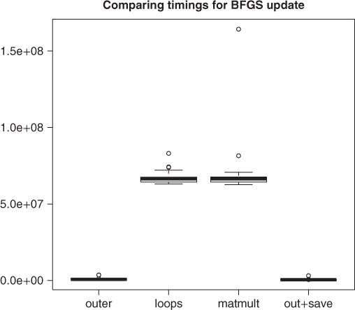
Figure 18.1
18.3 More speedups of R computations
We have just seen one example of how we might improve the speed of a function by substituting equivalent code. We will return to this shortly, but first will consider the byte-code compiler for R.
18.3.1 Byte-code compiled functions
One of the easiest tools for speeding up R is the so-called byte-code compiler due to Luke Tierney, which has been part of the standard distribution since version 2.14. There is also just-in-time compilation in the Ra system due to Stephen Milborrow (http://www.milbo.users.sonic.net/ra/), but I so far have no experience with that.
The treatment here will be limited to the use of the cmpfun() function, but readers who must squeeze every unnecessary microsecond out of their code should read the manual and run timing experiments. Furthermore, it is important to note that this facility can be very helpful, but my experience, echoing comments from Tierney and others, is that code using vectorized commands and functions like crossprod() or involving unsubscripted vectors will see little or no improvement. Code with vector element operations generally benefits quite substantially.
The compiler package is part of the distribution but needs to be loaded or invoked via appropriate instructions when packages are installed. Here we will use it explicitly. The compiler can be loaded, and the manual displayed, by R commands
require(compiler)
?compile
Note that it is possible to use this implicitly, so that functions are compiled as loaded. Sometimes the byte-code compiler is referred to as a “just-in-time” compiler, because R can, with appropriate options set, apply the compiler to code that is loaded via the source() command. My preference is to run things explicitly.
18.3.2 Avoiding loops
In R, the folklore is that loops are particularly “slow.” Moreover, while loops are considered slower than for loops. We can check that suggestion and in the process demonstrate the byte-code compilation possibility.
# forwhiletime.R
require(microbenchmark)
require(compiler)
tfor <- function(n) {
    for (i in 1:n) {
        xx <- exp(sin(cos(as.double(i))))
    }
    xx
}
twhile <- function(n) {
    i <- 0
    while (i < n) {
        i <- i + 1
        xx <- exp(sin(cos(as.double(i))))
    }
    xx
}
n <- 10000
timfor <- microbenchmark(tfor(n))
timwhile <- microbenchmark(twhile(n))
tforc <- cmpfun(tfor)
twhilec <- cmpfun(twhile)
timforc <- microbenchmark(tforc(n))
timwhilec <- microbenchmark(twhilec(n))
looptimes <- data.frame(timfor$time, timforc$time, timwhile$time, timwhilec$time)
colMeans(looptimes)
##    timfor.time   timforc.time  timwhile.time timwhilec.time
##       12883398        9177664       19394950       10354892
We observe that for loops take less than two-third the time of while loops in interpreted code but are only about 10% faster when that code is compiled. Moreover, the while loops gain a lot from compilation.
As indicated, R does best at computations that involve vectors, so that loops are not used explicitly. That is, when we can write an operation so that whole vectors undergo the same process, R generally performs well. Thus, sum(x * y) where x and y are vectors is fast. Similarly, crossprod() is efficient (but outputs a matrix structure). Loops or matrix multiplications (using %*%) are much slower. If we need to speed things up, it is important to run timings and to do so in the computing environment we will actually be using. The examples in this chapter are illustrations.
18.3.3 Package upgrades - an example
A general mantra among those who advise others about R is to use the latest versions of R and of packages. Owing to a rather unusual computational model, R can sometimes perform some operations very efficiently (from the point of view of machine cycles), but others can have unusually long execution times. For example, in 2011, I commented that I had two variants of a differential equation model I was trying to estimate by maximum likelihood, and one of these took almost 800 times as long to compute as the other. See the original post and follow the thread from http://tolstoy.newcastle.edu.au/R/e15/devel/11/08/0373.html. Such differences, when both codes are “reasonable” to an initial view, can be very annoying for users and can lead to criticism of R that is incorrect in a global sense, although clearly valid for the particular examples.
As I was about to put this example here, I had occasion to review the e-mail discussion referenced earlier. As I did a Google search, I also found a slightly later contribution by Martin Maechler, noting a new version of package expm. There are also more recent versions of package Matrix. Using the latest CRAN offerings in July 2013, I was not able to reproduce the extreme differences in timing that were observed in 2011. The data and the code to compute the two negative log likelihoods are as follows, along with some checks on the results obtained. Note that we execute this code off-line on a particular machine (J6) to keep the timings consistent.
require(expm)
## Loading required package: expm
## Loading required package: Matrix
##
## Attaching package: 'expm'
##
## The following object is masked from 'package:Matrix':
##
##    expm
tt <- c(0.77, 1.69, 2.69, 3.67, 4.69, 5.71, 7.94, 9.67, 11.77, 17.77, 23.77,
      32.77, 40.73, 47.75, 54.9, 62.81, 72.88, 98.77, 125.92, 160.19, 191.15,
      223.78, 287.7, 340.01, 340.95, 342.01)
y <- c(1.396, 3.784, 5.948, 7.717, 9.077, 10.1, 11.263, 11.856, 12.251,
     12.699, 12.869, 13.048, 13.222, 13.347, 13.507, 13.628, 13.804, 14.087,
     14.185, 14.351, 14.458, 14.756, 15.262, 15.703, 15.703, 15.703)
ones <- rep(1, length(t))
Mpred <- function(theta) {
    # WARNING: assumes tt global
    kvec <- exp(theta[1:3])
    k1 <- kvec[1]
    k2 <- kvec[2]
    k3 <- kvec[3]
    # MIN problem terbuthylazene disappearance
    z <- k1 + k2 + k3
    y <- z * z - 4 * k1 * k3
    l1 <- 0.5 * (-z + sqrt(y))
    l2 <- 0.5 * (-z - sqrt(y))
    val <- 100 * (1 - ((k1 + k2 + l2) * exp(l2 * tt) - (k1 + k2 + l1)              * exp(l1 * tt))/(l2 - l1))
}  # val should be a vector if t is a vector
negll <- function(theta) {
    # non expm version JN 110731
    pred <- Mpred(theta)
    sigma <- exp(theta[4])
    -sum(dnorm(y, mean = pred, sd = sigma, log = TRUE))
}
nlogL <- function(theta) {
    k <- exp(theta[1:3])
    sigma <- exp(theta[4])
    A <- rbind(c(-k[1], k[2]), c(k[1], -(k[2] + k[3])))
    x0 <- c(0, 100)
    sol <- function(tt) {
        100 - sum(expm(A * tt) %*% x0)
    }
    pred <- sapply(tt, sol)
    -sum(dnorm(y, mean = pred, sd = sigma, log = TRUE))
}
mytheta <- c(-2, -2, -2, -2)
vnlogL <- nlogL(mytheta)
cat("nlogL(-2,-2,-2,-2) = ", vnlogL, "
")
## nlogL(-2,-2,-2,-2) =  3292470
vnegll <- negll(mytheta)
cat("negll(-2,-2,-2,-2) = ", vnegll, "
")
## negll(-2,-2,-2,-2) =  3292470
We now have two ways to compute the negative log likelihood, nlogL() and negll(). We have, furthermore, checked that they give the same answer for a set of parameters. The nlogL() function uses the expm() exponential matrix function, which is notationally very convenient but notoriously difficult to compute reliably (Moler and Loan, 2003). There are two sets of tools in R to compute it, one in the Matrix package and the other in the package expm that has several approaches (we will use the default chosen by each package). tve
##                time.nlogL time.negll    ratio
## regular          55612122    25497.7 2181.067
## compiled         55412567    25679.3 2157.869
## regular +expm    14615661    26292.7  555.884
## compiled+expm    14571569    26148.5  557.262
While it is clear that the expm code is much more efficient than that in Matrix, avoiding the matrix exponential is a very very good idea if we want an efficient computation. Moreover, in this case, we see very little benefit from the compiler.
18.3.4 Specializing codes
We have mentioned in Chapter 11 that bounds constraints are very useful for the reliability and usefulness of function minimization programs. However, we should note that the bounds constraint feature does not come for free. In my packages Rvmmin and Rcgmin, I check for bounds and then call separate functions for the bounded or unconstrained cases. Let us check on a problem that is unconstrained whether this is worthwhile.
require(microbenchmark)
require(Rvmmin)
require(Rcgmin)
sqs <- function(x) {
    sum(seq_along(x) * (x - 0.5 * seq_along(x))^2)
}
sqsg <- function(x) {
    ii <- seq_along(x)
    g <- 2 * ii * (x - 0.5 * ii)
}
xstrt <- rep(pi, 20)
lb <- rep(-100, 20)
ub <- rep(100, 20)  # very loose bounds
bdmsk <- rep(1, 20)  # free parameters
tvmu <- microbenchmark(avmu <- Rvmminu(xstrt, sqs, sqsg))
tcgu <- microbenchmark(acgu <- Rcgminu(xstrt, sqs, sqsg))
tvmb <- microbenchmark(avmb <- Rvmminb(xstrt, sqs, sqsg, bdmsk = bdmsk, lower = lb, upper = ub))
tcgb <- microbenchmark(acgb <- Rcgminb(xstrt, sqs, sqsg, bdmsk = bdmsk, lower = lb, upper = ub))
svmu <- summary(tvmu$time)
cnames <- names(svmu)
svmu <- as.numeric(svmu)
svmb <- as.numeric(summary(tvmb$time))
scgu <- as.numeric(summary(tcgu$time))
scgb <- as.numeric(summary(tcgb$time))
names(svmu) <- cnames
names(svmb) <- cnames
names(scgu) <- cnames
names(scgb) <- cnames
mytab <- rbind(svmu, svmb, scgu, scgb)
rownames(mytab) <- c("Rvmminu", "Rvmminb", "Rcgminu", "Rcgminb")
# dput(mytab, file='includes/C18mytabJ6.dput')
ftable(mytab)
##              Min.  1st Qu.   Median     Mean  3rd Qu.     Max.
##
## Rvmminu   5621000  5738000  5844000  6290000  7060000  8447000
## Rvmminb  26590000 28160000 28470000 28680000 28930000 49850000
## Rcgminu   2466000  2517000  2557000  2723000  2604000  6137000
## Rcgminb  23270000 24020000 24790000 24780000 25180000 30120000
We see that the bounds constrained versions of the codes are four to nine times slower on this simple function, where we can anticipate that the bounds were never active.
18.4 External language compiled functions
We can also consider interfacing our optimizers to objective functions compiled in other computing languages. While interfacing R to a Fortran, C, or other compiled-code optimizer is relatively tedious and involved, using a compiled objective function in such languages is quite easy. To illustrate this, let us use the minimization of the Rayleigh quotient to find the largest eigenvalue of a symmetric matrix. The example we will use is the Moler matrix from Appendix 1 of Nash (1979), which is defined in the following code.
molermat <- function(n) {
    A <- matrix(NA, nrow = n, ncol = n)
    for (i in 1:n) {
        for (j in 1:n) {
            if (i == j)
                A[i, i] <- i else A[i, j] <- min(i, j) - 2
        }
    }
    A
}
rayq <- function(x, A) {
    rayquo <- as.numeric(crossprod(x, crossprod(A, x))/crossprod(x))
}
We will also compute the eigensolutions of the Moler matrix using R's function eigen(), which finds all eigenvalues and eigenvectors.
require(microbenchmark)
require(compiler)
molermatc <- cmpfun(molermat)
rayqc <- cmpfun(rayq)
n <- 200
x <- rep(1, n)
tbuild <- microbenchmark(A <- molermat(n))$time
tbuildc <- microbenchmark(A <- molermatc(n))$time
teigen <- microbenchmark(evs <- eigen(A))$time
tr <- microbenchmark(rayq(x, A))$time
trc <- microbenchmark(rayqc(x, A))$time
eigvec <- evs$vectors[, 1]  # select first eigenvector
# normalize first eigenvector
eigvec <- sign(eigvec[[1]]) * eigvec/sqrt(as.numeric(crossprod(eigvec)))
The timings are summarized below in Section 18.4.2, showing that building the matrix takes a considerable computational effort and can be made quicker with the byte compiler. However, the speedup in the evaluation of the Rayleigh quotient with the byte compiler is negligible.
Once we have matrix A, we can try finding the maximum eigensolution by minimizing the Rayleigh quotient for matrix -A. To make the eigenvectors comparable between solution methods, we need to normalize them. I have chosen to scale the eigenvector so the sum of squares of the its components is 1 and the first component is positive. We compare the eigenvalue and vector with the comparable result from eigen().
Anticipating the timings we report later based on the time we must wait for the optimization to run, it is clear that this approach to the eigensolution is not competitive in timing with eigen().
require(optimx)
tcg <- system.time(amax <- optimx(x, fn = rayq, method = "Rcgmin", control = list(usenumDeriv = TRUE,
    kkt = FALSE), A = -A))[[3]]
# summary(amax)
cat("maximal eigensolution: Value=", -amax$value, "  timecg= ", tcg, "
")
tvec <- coef(amax)[1, ]
rcgvec <- sign(tvec)[[1]] * (tvec)/sqrt(as.numeric(crossprod(tvec)))
cat("Compare with eigen()
")
cat("Difference in eigenvalues = ", (-amax$value[1] - evs$values[[1]]), "
")
cat("Max abs vector difference = ", max(abs(eigvec - rcgvec)), "
")
We could use the byte compiler on the function rayq(), but I found very little advantage in so doing. Possibly as ![]() gets larger, the advantage of the compiled code could be more pronounced. This is using an explicit matrix
gets larger, the advantage of the compiled code could be more pronounced. This is using an explicit matrix A. Given that we know the matrix elements, we could implicitly perform the matrix multiplication. Here is the code to do that.
axmoler <- function(x) {
    # A memory-saving version of A%*%x For Moler matrix.
    n <- length(x)
    j <- 1:n
    ax <- rep(0, n)
    for (i in 1:n) {
        term <- x * (pmin(i, j) - 2)
        ax[i] <- sum(term[-i])
    }
    ax <- ax + j * x
    ax
}
require(compiler)
require(microbenchmark)
n <- 200
x <- rep(1, n)
tax <- microbenchmark(ax <- axmoler(x))$time
axmolerc <- cmpfun(axmoler)
taxc <- microbenchmark(axc <- axmolerc(x))$time
cat("time.ax, time.axc:", mean(tax), mean(taxc), "
")
## On J6 gives time.ax, time.axc: 5591866 4925221
Again, the byte compiler is not making a lot of difference, although we have avoided storing a large matrix. Of itself, using an implicit multiplication in R may not be helpful for speeding up computations. The issue is that we have to essentially create the matrix each time we do a matrix–vector product. However, if we embed such a computation in a faster computing environment, we do get some gains. Let us look at running the matrix–vector and the Rayleigh quotient calculations in Fortran.
18.4.1 Building an R function using Fortran
While we show Fortran here, the same general approach will hold for C or other compatible compiled languages.
First, we need to write a Fortran subroutine because R can only call routines with a void return. Here is an example subroutine that multiplies a vector x by the Moler matrix implicitly giving the result in vector ax. It then computes the Rayleigh quotient, returning the result in the argument variable rq.
c     This is file rqmoler.f
      subroutine rqmoler(n, x, rq)
      integer n, i, j
      double precision x(n), ax(n), sum, rq
c     return rq = t(x) * A * x / (t(x) * x)  for A = moler matrix
c     A[i,j]=min(i,j)-2 for i<>j, or i for i==j
      do 20 i=1,n
         sum=0.0
         do 10 j=1,n
            if (i.eq.j) then
               sum = sum+i*x(i)
            else
               sum = sum+(min(i,j)-2)*x(j)
            endif
 10      continue
         ax(i)=sum
 20   continue
      rq=0.0
      sum=0.0
      do 30 i=1,n
         rq = rq+ax(i)*x(i)
         sum = sum + x(i)**2
 30   continue
      rq = rq/sum
      return
      end
Second, we need to build the dynamic load library. R provides a tool for this that is run from the command line as follows.
R CMD SHLIB rqmoler.f
This will create files rqmoler.o and rqmoler.so in the working directory for Linux/Unix systems. On Microsoft Windows machines (I have only tested this in a Windows XP virtual machine), the user must open a command window and issue the same command to create a dynamic link library file rqmoler.dll. As far as I can determine, the Rtools collection by Duncan Murdoch is sufficient for this task.
We now need to load this routine into our R session, which is done with
dyn.load("rqmoler.so")
## In Windows dyn.load("rqmoler.dll")
cat("Is the Fortran RQ function loaded ",is.loaded('rqmoler'),"
")
and we check that the Fortran routine is available using the is.loaded() function. Note that we leave off the filename suffix.
The function “rqmoler” takes a vector x and returns the Rayleigh quotient. But it is important to note that we do not need the matrix A at all. Note that the Fortran rqmoler.f returns a list of elements n, x, and rq, where the last item is the result we want.
dyn.load("/home/john/nlpor/supportdocs/tuning/rqmoler.so")
cat("Is the Fortran RQ function loaded? ", is.loaded("rqmoler"), "
")
## Is the Fortran RQ function loaded?  TRUE
We need to get the negative of the Rayleigh quotient for our maximal Eigensolution and then optimize it, which we do with the following code.
frqmoler <- function(x) {
    n <- length(x)
    rq <- 0
    res <- .Fortran("rqmoler", n = as.integer(n), x = as.double(x), rq = as.double(rq))
    res$rq
}
nfrqmoler <- function(x) {
    (-1) * frqmoler(x)
}
tcgrf <- system.time(amaxi <- optimx(x, fn = nfrqmoler, method = "Rcgmin", control = list(usenumDeriv = TRUE,
    kkt = FALSE, trace = 1)))[[3]]
18.4.2 Summary of Rayleigh quotient timings
Noting that these examples are, of course, just examples, let us look at the timings for different tasks in the Rayleigh quotient minimization for the Moler matrix of dimension 200 on our machine named J6
- In R, just building the Moler matrix of order 200 takes on average 147.857 ms, but the byte compiler reduces this dramatically to 42.787 ms.
- Our main comparison is with the function
eigen(), which computes all eigensolutions in a mean time of 30.614 ms. This is very fast and hard to beat. Note that the overall time should add in the “build” if we compare with methods that develop the matrix implicitly. - Once we have the matrix
A, then computing the Rayleigh quotient in R takes an average of 0.215 ms, interpreted, or 0.201 ms, byte compiled. - If we use the Moler matrix implicitly to compute the Rayleigh quotient in R, this takes an average of 5.602 ms, interpreted, or 5.291 ms, byte compiled.
- Using a Fortran version of the Rayleigh quotient called through
frqmoler(), where the matrix is generated implicitly takes about 0.083 ms. For compatibility with a calling program that specifies the matrix, I actually tested a version of this with the matrix in the argument list but found almost identical timings. That is, I specifiedfrqmolerA<-function(x, A)
in a definition otherwise identical to function
frqmoler(). The matrix is, of course, not used. The Fortran function is over 60 times faster than the R one using an implicit matrix. Ignoring the building time, it is still better than double the time using an explicit matrix. - To minimize the Rayleigh quotient for the maximal eigenvalue takes quite a long time, indeed over 4 s (not milliseconds) using the explicit matrix form and, worse, nearly 50 s with the implicit Rayleigh quotient. We do better with the Fortran implicit version but still take over 1 s. And this is to get just a single eigensolution, where
eigen()gets them all in about 30 ms.
From the above, it may appear that minimizing the Rayleigh quotient is unsuitable for computing eigensolutions. In general I would agree, but there are specialized minimization tools (Geradin, 1971) that, coded in Fortran or some other fast computational environment, do very well. However, such a method is unlikely to be a choice of R users.
It is worth noting that each situation that must be speeded up requires at least some individual attention. From a more extensive set of timings, now over a year old, I will venture the following generalizations:
- A matrix–vector multiplication function that implicitly performs the operation can be written so that no actual matrix is needed. This saves a great deal of memory when the order of the matrix gets large, but for the Moler matrix uses element operations. This gains from compilation either with
cmpfunor with an external language such as Fortran. However, the R version of implicit matrix–vector routine is much slower than the Fortran one. - Compilation with
cmpfun()provides quite decent time reductions for building the matrix (molermat). That is, compilation helps reduce operations on elements of vectors and matrices. However, these operations remain relatively slow in R. - Compiling an optimizer like
spgfrom packageBBthat already is vector oriented and gave almost negligible speedup.
Both Ravi Varadhan and Gabor Grothendieck provided valuable input to the work that underlies the discussion of the Rayleigh quotient problem.
18.5 Deciding when we are finished
One of the major parts of any iterative algorithm is deciding when it is finished, or rather when the approximation to the answer we have is “good enough.” In Chapter 17, we considered various conditions that good optimization solutions should satisfy. These are mainly that the gradient or some measure thereof is “small,” while the surface around the solution curves upwards. Actually computing such tests, as we saw, can be computationally demanding, so within optimization codes we often look for proxies for the actual gradient and particularly for Hessian information.
As mentioned in Chapter 2, gradient methods generally stop when the norm of the gradient is small. While some developers are happy to use the gradient projection along the current search direction for this measure, I like to revert to the steepest descents direction and stop only when no progress can be made with that as our search vector. However, this does sometimes cause extra work to be performed that is not necessary.
Note that bounds or other constraints render the termination tests more complicated, as we must first project our search onto the constraint surface. For bounds, the changes are relatively simple but do need care. Surprisingly, masks, for which the changes to code are almost trivial, seem to be rarely offered in optimizer codes. In R we need to recognize that both bounds and masks involve individual matrix or vector elements and may degrade performance compared to fully vectorized codes.
One of the major decisions that developers must make is “how small is zero” in a particular problem. Choosing tolerances too small will make an algorithm try very hard to reduce the objective function and use unnecessary computational effort. But tolerances that are too large risk returning “solutions” that are far from a true optimum. My own preference is to err on the side of caution and make the tolerances rather strict. Users who really understand their problem can relax the tolerances.
Mostly I prefer to avoid tolerances, as users are prone to change them and then complain to me that “your program doesn't work” because it has stopped well before it has finished and stopped because they changed the tolerance. Therefore, I often will test for “no change” in numbers by testing for equality between ![]() and
and ![]() where offset is a modest number of the order of 100 to 10 000 for regular
where offset is a modest number of the order of 100 to 10 000 for regular double numbers. When ![]() and
and ![]() are small, the numbers compared eventually become just the value of offset, while when
are small, the numbers compared eventually become just the value of offset, while when ![]() and
and ![]() are quite large, we are comparing their most significant digits. Users generally do not tinker with the offset, as it does not appear to be a form of tolerance.
are quite large, we are comparing their most significant digits. Users generally do not tinker with the offset, as it does not appear to be a form of tolerance.
If the methods are entirely coded in R, users can modify the actual R code of the termination tests if they must solve many similar problems. I advise this to be investigated if there could be benefits in a production-type environment. Additionally, the entire objective and optimizer may be implemented in a compiled language and called from R as above. R can still provide convenience in loading and transforming data and in drawing graphs of data or results.
For exploratory and interactive work, I generally advise very tight tolerances. The reason for this is to force optimizers to strive for the best answer possible, but it comes at the price of some, possibly many, extra iterations and function and gradient evaluations. My own codes tend to rather aggressive tolerances and I believe that they mostly do much more work than they need. On the other hand, if they can continue to reduce the objective in approaching a solution, they do.
18.5.1 Tests for things gone wrong
Sometimes a calculation is “finished” because the user has supplied some input that is inappropriate for the situation. “NA” values (missing data) may be acceptable in some situations but is rarely appropriate for parameters of objective functions. Similarly, if the initial function value computation is attempted at an inadmissible point, for example, where there is a zero divide or square root of a negative number, then there is no sense in proceeding. However, within the optimization, as we have noted in Chapter 3, trial sets of parameters that are inadmissible may be generated. In some methods, we may be able to recognize this situation and continue with the optimization. However, when progress is not possible, we need to terminate with notification to the user. See section 3.7.
optplus included a number of checks that our objective function returns suitable results. We want a numeric scalar result. Some optimizers will still “work” with other objective function types, but the ultimate answers could be unreliable. Unfortunately, carrying out all these tests takes time. In fact, it takes so much time that I have set aside that direction of development for my optimization tools. Moreover, if you can ensure the inputs to functions are appropriate, then it is worth looking into how you can bypass such checks.
It is worth noting that a particular case that has caused trouble over the years is the occurrence of objects that are effectively 1 ![]() 1 matrices. These behave “mostly” like scalar numbers in computations, but there are enough functions that cannot deal with them to get us into trouble. If in doubt, convert these to numbers with the
1 matrices. These behave “mostly” like scalar numbers in computations, but there are enough functions that cannot deal with them to get us into trouble. If in doubt, convert these to numbers with the as.numeric() function. More generally, many functions that deal with matrices or vectors are not set up to deal with the ![]() situation.
situation.
From the above, you may correctly surmise that a modest level of paranoia is useful when writing our objective functions and code to launch the optimizations, as errors creep in very easily.
References
- Dongarra JJ, Luszczek P, and Petitet A 2003 The LINPACK benchmark: past, present, and future. Concurrency and Computation: Practice and Experience 15(9), 803–820.
- Eugster MJA and Leisch F 2011 Exploratory analysis of benchmark experiments—an interactive approach. Computational Statistics 26(4), 699–710.
- Eugster MJA, Hothorn T, and Leisch F 2012 Domain-based benchmark experiments: exploratory and inferential analysis. Austrian Journal of Statistics 41(1), 5–26.
- Geradin M 1971 The computational efficiency of a new minimization algorithm for eigenvalue analysis. Journal of Sound and Vibration 19, 319–331.
- Kusnierczyk W 2012 rbenchmark: Benchmarking routine for R. R package version 1.0.0.
- Mersmann O 2013 microbenchmark: sub microsecond accurate timing functions. R package version 1.3-0.
- Moler C and Loan CV 2003 Nineteen dubious ways to compute the exponential of a matrix, twenty-five years later. SIAM Review 45(1), 3–49.
- Nash JC 1979 Compact Numerical Methods for Computers: Linear Algebra and Function Minimisation. Adam Hilger, Bristol. Second Edition, 1990, Bristol: Institute of Physics Publications.