5.1 The optimize() function

R has a built-in function to find the minimum of a function of a single parameter in a given interval . This is optimize(). It requires a function or expression to be supplied, along with an interval specified as a two-element vector, as in the following example. The method is based on the work by Brent (1973).

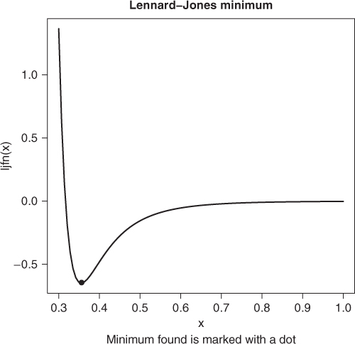
A well-known function in molecular dynamics is the Lennard–Jones 6–12 potential (http://en.wikipedia.org/wiki/Lennard-Jones_potential). Here we have chosen a particular form as the function is extremely sensitive to its parameters ep and sig. Moreover, the limits for the curve() have been chosen so that the graph is usable because the function has extreme scale changes (Figure 5.1). Let us see if we can find the minimum.

# The L-J potential function
ljfn <- function(r, ep = 0.6501696, sig = 0.3165555) {
    fn <- 4 * ep * ((sig/r)^12 - (sig/r)^6)
}
min <- optimize(ljfn, interval = c(0.001, 5))
print(min)

## $minimum
## [1] 0.35531
##
## $objective
## [1] −0.65017
## Now graph it
curve(ljfn, from = 0.3, to = 1)
points(min$minimum, min$objective, pch = 19)
title(main = "Lennard Jones minimum")
title(sub = "Minimum found is marked with a dot")

Later, in Chapter 11, we will see a way to use optimize() in a way that avoids the dangers of a zero-divide.

5.2 Using a root-finder

As we have seen in Chapter 4, if we have functional form of the derivative of ljfn, we can attempt to solve for the root of this function and thereby hope to find an extremum of the original function. This does not, of course, guarantee that we will find a minimum, because the gradient can be zero at a maximum or saddle point. Here we use uniroot, but any of the ideas from Chapter 4 can be used.

ljgr <- function(r, ep = 0.6501696, sig = 0.3165555) {
    expr1 <- 4 * ep
    expr2 <- sig/r
    expr8 <- sig/r^2
    value <- expr1 * (expr2^12 - expr2^6)
    grad <- -(expr1 * (12 * (expr8 * expr2^(11)) - 6 * (expr8 * expr2^5)))
}
root <- uniroot(ljgr, interval = c(0.001, 5))
cat("f(", root$root, ")=", root$f.root, " after ", root$iter, " Est. Prec'n=",
    root$estim.prec, "
")
## f( 0.3553 )= -0.0079043  after  13  Est. Prec'n= 6.1035e-05

5.3 But where is the minimum?

This is all very good, but most novices to minimization soon realize that they need to provide an interval to get a sensible answer. In many problems—and most of the ones I have had to work with—this is the hard part of getting an answer. Consider the following example (Figure 5.2).

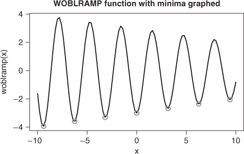
woblramp <- function(x) {
    (-3 + 0.1 * x) * cos(x * 2)
}
require(pracma, quietly = TRUE)
wmins <- findmins(woblramp, a = -10, b = 10)
curve(woblramp, from = -10, to = 10)
ymins <- woblramp(wmins)  # compute the function at minima
points(wmins, ymins, col = "red")  # and overprint on graph
title(main = "WOBLRAMP function with minima graphed")

An approach to this is to perform a grid search on the function. That is what Borchers (2013) does with function findmins from package pracma. Another approach is to use the base R function curve and simply draw the function between two values of the argument, which we did earlier. Indeed, drawing a 1D function is natural and well advised as a first step. We will then soon discover those nasty scaling issues that get in the way of automated solutions of problems of this sort.

In the earlier example, I considered issuing the require statement without the quietly=TRUE condition. This directive generally suppresses message about the replacement of function already loaded with those of the same name in pracma. The following is an example showing that possibility.

detach(package:pracma)
require(numDeriv)
## Loading required package: numDeriv
require(pracma)
## Loading required package: pracma
##
## Attaching package: 'pracma'
##
## The following objects are masked from 'package:numDeriv':
##
##    grad, hessian, jacobian

I believe the confusion of functions that have the same name is quite often a source of trouble for users of R. If one is in doubt, it is possible to invoke functions using the form

packagename::functionname()

and I recommend this rather cumbersome approach if there is any suspicion that there may be confusion.

5.4 Ideas for 1D minimizers

The literature of both root-finding and minimization of functions of one parameter was quite rich in the 1960s and 1970s. Essentially, developers have sought to

• provide a robust method that will find at least the minimum of a unimodal function, and hopefully one minimum of a multimodal function, when given a starting interval for the parameter;
• be fast, that is, use few function and/or derivative evaluations when the function is “well behaved;”
• be relatively easy to implement.

To this end, the methods try to meld robust searches such as success–failure search (Dixon, 1972), Golden-section search (http://en.wikipedia.org/wiki/Golden_section_search), or bisection (http://en.wikipedia.org/wiki/Bisection_method) with an inverse interpolation based on a simple polynomial model, usually a quadratic. One of the most popular is that of Brent (1973), called FMIN.

For most users, even those with quite complicated functions, 1D minimization is not likely to require heroic efforts to improve efficiency. When there are thousands of problems to solve, then it is perhaps worth looking at the method(s) a bit more closely. In such cases, good starting value estimates and customized termination tests may do more to speed up the computations than changing method.

On the other hand, the method requirements may be important. The Brent/Dekker codes ask us to specify an interval for the parameter of interest. A code using the success/failure search (generally followed by quadratic inverse interpolation) uses a starting point and a step for the parameter of interest. These different approaches force the user to provide rather different information. If we have a function that involves fairly straightforward computations, but no idea of the location of the minimum, then the “point + step” formulation is much less demanding in my experience, because we do not need to worry that we have bracketed a minima.

One matter that users must keep in mind is that many functions are not defined for the entire domain of the parameter. For example, consider the function

5.1

This function is undefined for nonpositive. It is likely sensible for the user to add a test for this situation and return a very large value for the function. This will avoid trouble but may slow down the methods. Note that the R function optimize() does seem to have such protection built-in, but users should not count on such careful coding of minimizers. The following is an illustration of how to provide the protection.

# Protected log function
mlp <- function(x) {
    if (x < 1e-09)
        fval <- 0.1 * .Machine$double.xmax else fval <- (log(x) * (x * x - 3000))
}
ml <- function(x) {
    fval <- (log(x) * (x * x - 3000))
}
min <- optimize(mlp, interval = c(-5, 5))
print(min)
## $minimum
## [1] 4.9999
##
## $objective
## [1] -4788
minx <- optimize(ml, interval = c(-5, 5))
## Warning: NaNs produced
## Warning: NA/Inf replaced by maximum positive value
print(minx)
## $minimum
## [1] 4.9999
##
## $objective
## [1] -4788
## But we missed the solution!
min2 <- optimize(mlp, interval = c(-5, 55))
print(min2)
## $minimum
## [1] 20.624
##
## $objective
## [1] -7792.1

The failure of optimize() to tell us that the minimum has not been found is a weakness that I believe is unfortunate. We can easily check if the function has a small gradient. However, it is also suspicious that the reported minimum is at the limit of our supplied interval.

Adding better safeguards to a version of optimize() is one of the tasks on my “to do” list.

5.5 The line-search subproblem

One-dimensional minimization occurs very frequently in multiparameter optimizations, where a subproblem is to find “the minimum” of the function along a search direction from a given point. In practice, because the search direction is likely to be imperfect, a precise minimum along the line may not be required, and many line-search subprocesses seek only to provide a satisfactory improvement. Note also that the “point + step” formulation is more convenient than the interval start approach for the line search, although interval approaches may have their place in trust region methods where there is a limit to how far we want to proceed along a particular search direction.

References

1. Borchers HW 2013 pracma: Practical Numerical Math Functions. R package version 1.5.0.
2. Brent R 1973 Algorithms for Minimization without Derivatives. Prentice-Hall, Englewood Cliffs, NJ.
3. Dixon L 1972 Nonlinear Optimisation. The English Universities Press Ltd., London.