
Chapter 6
Nonlinear least squares
As we have mentioned, the nonlinear least squares problem is sufficiently common and important that special tools exist for its solution. Let us look at the tools R provide either in the base system or otherwise for its solution.
6.1 nls() from package stats
In the commonly distributed R system, the stats package includes nls(). This function is intended to solve nonlinear least squares problems, and it has a large repertoire of features for such problems. A particular strength is the way in which nls() is called to compute nonlinear least squares solutions. We can specify our nonlinear least squares problem as a mathematical expression, and nls() does all the work of translating this into the appropriate internal computational structures for solving the nonlinear least squares problem. In my opinion, nls() points the way to how nonlinear least squares and other nonlinear parameter estimation should be implemented and is a milestone in the software developments in this field. Thanks to Doug Bates and his collaborators for this.
nls() does, unfortunately, have a number of shortcomings, which are discussed in the following text. We also show some alternatives that can be used to overcome the deficiencies.
6.1.1 A simple example
Let us consider a simple example where nls() works using the weight loss of an obese patient over time (Venables and Ripley, 1994, p. 225) (Figure 6.1). The data is in the R package MASS that is in the base distribution under the name wtloss. I have extracted that here so that it is not in a separate file from the manuscript.
Weight <- c(184.35, 182.51, 180.45, 179.91, 177.91, 175.81, 173.11, 170.06, 169.31,
    165.1, 163.11, 158.3, 155.8, 154.31, 153.86, 154.2, 152.2, 152.8, 150.3, 147.8,
    146.1, 145.6, 142.5, 142.3, 139.4, 137.9, 133.7, 133.7, 133.3, 131.2, 133, 132.2,
    130.8, 131.3, 129, 127.9, 126.9, 127.7, 129.5, 128.4, 125.4, 124.9, 124.9, 118.2,
    118.2, 115.3, 115.7, 116, 115.5, 112.6, 114, 112.6)
Days <- c(0, 4, 7, 7, 11, 18, 24, 30, 32, 43, 46, 60, 64, 70, 71, 71, 73, 74, 84,
    88, 95, 102, 106, 109, 115, 122, 133, 137, 140, 143, 147, 148, 149, 150, 153,
    156, 161, 164, 165, 165, 170, 176, 179, 198, 214, 218, 221, 225, 233, 238, 241,
    246)
wl <- data.frame(Weight = Weight, Days = Days)
wlmod <- "Weight ∼ b0 + b1*2^(-Days/th)"
wlnls <- nls(wlmod, data = wl, start = c(b0 = 1, b1 = 1, th = 1))
summary(wlnls)
##
## Formula: Weight ∼ b0 + b1 * 2^(-Days/th)
##
## Parameters:
##    Estimate Std. Error t value Pr(>|t|)
## b0    81.37       2.27    35.9   <2e-16 ***
## b1   102.68       2.08    49.3   <2e-16 ***
## th   141.91       5.29    26.8   <2e-16 ***
## - - -
## Signif. codes:  0 '***' 0.001 '**' 0.01 '*' 0.05 '.' 0.1 ' ' 1
##
## Residual standard error: 0.895 on 49 degrees of freedom
##
## Number of iterations to convergence: 6
## Achieved convergence tolerance: 3.28e-06
plot(wl$Days, wl$Weight)
title("Weight loss over time in Days")
points(wl$Days, predict(wlnls), type = "l", col = "red")
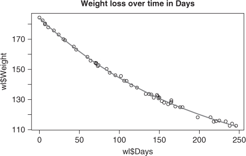
Despite a very crude set of starting parameters, we see that in this case nls() has done a good job of fitting the model to the data.
6.1.2 Regression versus least squares
It is my belief that nls() is mistitled “nonlinear least squares.” Its main purpose is to solve nonlinear regression modeling problems, where we are trying to estimate the parameters of models by adjusting them to fit data. In such problems, we rarely get a zero or even a particularly small sum of squares. Moreover, we are often interested in the variability of the parameters, also referred to as coefficients, and quantities computed from them. It is worth keeping this in mind when comparing tools for the nonlinear least squares problem. That nonlinear least squares tools are used for nonlinear regression is obvious. That not all nonlinear least squares problems arise from regression applications may be less clear depending on the history and experience of the user.
6.2 A more difficult case
Let us now try an example initially presented by Ratkowsky (1983, p. 88) and developed by Huet et al. (1996, p. 1). This is a model for the regrowth of pasture, with yield as a function of time since the last grazing. Units were not stated for either variable, which I consider bad practice, as units are important information to problems (Nash, 2012). (The criticism can also be made of my own Hobbs Example 1.2. Sometimes the analyst is not given all the information.)
Once again, we set up the computation by putting the data for the problem in a data frame and specifying the formula for the model. This can be as a formula object, but I have found that saving it as a character string seems to give fewer difficulties. Note the ∼ (tilde) character that implies “is modeled by” to R. There must be such an element in the formula for nls() as well as for the package nlmrt, which we will use shortly.
We also specify two sets of starting parameters, that is, the ones, which is a trivial (but possibly unsuitable) start with all parameters set to 1, and huetstart, which was suggested in Huet et al. (1996) and is provided in the following in the code. However, for reasons that will become clear in the following text, we write the starting vector with the exponential parameters first.
options(width = 60)
pastured <- data.frame(time = c(9, 14, 21, 28, 42, 57, 63, 70, 79),
    yield = c(8.93,10.8, 18.59, 22.33, 39.35, 56.11, 61.73, 64.62, 67.08))
regmod <- "yield ∼ t1 - t2*exp(-exp(t3+t4*log(time)))"
ones <- c(t3 = 1, t4 = 1, t1 = 1, t2 = 1)  # all ones start
huetstart <- c(t3 = 0, t4 = 1, t1 = 70, t2 = 60)
Note that the standard nls() of R fails to find a solution from either start.
anls <- try(nls(regmod, start = ones, trace = FALSE, data = pastured))
print(strwrap(anls))
## [1] "Error in nlsModel(formula, mf, start, wts) : singular"
## [2] "gradient matrix at initial parameter estimates"
anlsx <- try(nls(regmod, start = huetstart, trace = FALSE, data = pastured))
print(strwrap(anlsx))
## [1] "Error in nls(regmod, start = huetstart, trace ="
## [2] "FALSE, data = pastured) : singular gradient"
Let us now try the routine nlxb() from package nlmrt. This function is designed as a replacement for nls(), although it does not cover every feature of the latter. Furthermore, it was specifically prepared as a more robust optimizer than those offered in nls(). nlxb() is more strict than nls() and requires that the problem data be in a data frame. We try both of the suggested starting vectors.
require(nlmrt)
anmrt <- nlxb(regmod, start = ones, trace = FALSE, data = pastured)
anmrt
## nlmrt class object: x
## residual sumsquares =  4648.1  on  9 observations
##     after  3    Jacobian and  4 function evaluations
##   name        coeff       SE      tstat     pval      gradient    JSingval
## t3          0.998202         NA        NA        NA   1.889e-08           3
## t4          0.996049         NA        NA        NA    4.15e-08   1.437e-09
## t1           38.8378         NA        NA        NA   -3.04e-11   2.167e-16
## t2           1.00007         NA        NA        NA  -7.748e-10    5.14e-26
anmrtx <- try(nlxb(regmod, start = huetstart, trace = FALSE,
    data = pastured))
anmrtx
## nlmrt class object: x
## residual sumsquares =  8.3759  on  9 observations
##     after  32    Jacobian and  44 function evaluations
##   name       coeff      SE      tstat      pval      gradient    JSingval
## t3          -9.2088    0.8172    -11.27  9.617e-05   5.022e-06       164.8
## t4          2.37778     0.221     10.76  0.0001202  -6.244e-05       3.762
## t1          69.9554     2.363     29.61  8.242e-07   2.196e-07       1.617
## t2          61.6818     3.194     19.31  6.865e-06  -7.295e-07      0.3262
The first result has such a large sum of squares that we know right away that there is not a good fit between the model and the data. However, note that the gradient elements are essentially zero, as are three out of four singular values of the Jacobian. The result anmrtx is more satisfactory, although interestingly the gradient elements are not quite as small as those in anmrt. Note that the gradient and Jacobian singular values are NOT related to particular coefficients, but simply displayed in this format for space efficiency.
The Jacobians at the starting points indicate why nls() fails. We use the nlmrt function model2jacfun() to generate the R code for the Jacobian, then we compute their singular values. In both cases, the Jacobians could be considered singular, so nls() is unable to proceed.
pastjac <- model2jacfun(regmod, ones, funname = "pastjac")
J1 <- pastjac(ones, yield = pastured$yield, time = pastured$time)
svd(J1)$d
## [1] 3.0000e+00 1.3212e-09 2.1637e-16 3.9400e-26
J2 <- pastjac(huetstart, yield = pastured$yield, time = pastured$time)
svd(J2)$d
## [1] 3.0005e+00 1.5143e-01 1.1971e-04 1.8584e-10
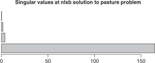
A useful way to demonstrate the magnitudes of the singular values is to put them in a bar chart (Figure 6.2). If we do this with the singular values from the result anmrtx, we find that the bar for the smallest singular value is very small. Indeed, the lion's share of the variability in the Jacobian is in the first singular value.
Jnmrtx <- pastjac(coef(anmrtx), yield = pastured$yield, time = pastured$time)
svals <- svd(Jnmrtx)$d
barplot(svals, main = "Singular values at nlxb solution to pasture problem",
    horiz = TRUE)
The Levenberg–Marquardt stabilization used in nlxb() avoids the singularity of the Jacobian by augmenting its diagonal until it is (computationally) nonsingular. The details of this common approach may be found elsewhere (Nash, 1979, Algorithm 23). The package minpack.lm has function nlsLM to implement a similar method and is able to solve the problem from the parameters huetstart, but because it uses an internal function nlsModel() from nls() to set up the computations, it is not able to get started from the values in the starting vector ones.
require(minpack.lm)
## Loading required package: minpack.lm
aminp <- try(nlsLM(regmod, start = ones, trace = FALSE, data = pastured))
summary(aminp)
##    Length     Class      Mode
##         1 try-error character
aminpx <- try(nlsLM(regmod, start = huetstart, trace = FALSE,
    data = pastured))
print(aminpx)
## Nonlinear regression model
##   model: yield ∼ t1 - t2 * exp(-exp(t3 + t4 * log(time)))
##    data: pastured
##    t3    t4    t1    t2
## -9.21  2.38 69.96 61.68
##  residual sum-of-squares: 8.38
##
## Number of iterations to convergence: 42
## Achieved convergence tolerance: 1.49e-08
Both nlmrt and minpack.lm have functions to deal with a model expressed as an R function rather than an expression, and nlmrt also has tools to convert an expression to a function. The package pracma has a similar function lsqnonlin(). CRAN package MarqLevAlg is also intended to solve unconstrained nonlinear least squares problems but works with the sum-of-squares function rather than the residuals.
There are some other tools for R that aim to solve nonlinear least squares problems, to the extent that there are two packages called nls2. At the time of writing (August 2013), we have not yet been able to successfully use the INRA package nls2. This is a quite complicated package and is not installable as a regular R package using install.packages(). The nls2 package on CRAN by Gabor Grothendieck is intended to combine a grid search with the nls() function. The following is an example of its use to solve the pasture regrowth problem starting at ones:
require(nls2)
## Loading required package: nls2
## Loading required package: proto
set.seed(123)  # for reproducibility
regmodf <- as.formula(regmod)  # just in case
m100 <- c(t1 = -100, t2 = -100, t3 = -100, t4 = -100)
p100 <- (-1) * m100
gstart <- data.frame(rbind(m100, p100))
anls2 <- try(nls2(regmodf, start = gstart, data = pastured, algorithm = "random-search", control = list(maxiter = 1000)))
print(anls2)
## Nonlinear regression model
##   model: yield ∼ t1 - t2 * exp(-exp(t3 + t4 * log(time)))
##    data: pastured
##    t1    t2    t3    t4
##  11.6 -44.8  84.8 -26.1
##  residual sum-of-squares: 1377
##
## Number of iterations to convergence: 1000
## Achieved convergence tolerance: NA
This is not nearly so good as our Marquardt solutions from nlxb() or nlsLM(), but trials with those routines from other starting points give “answers” that are all over the place. Something is not right!
We could, however, try the partial linearity tools in nls2(). We note that the parameter ![]() is an intercept and
is an intercept and ![]() multiplies the exponential construct involving
multiplies the exponential construct involving ![]() and
and ![]() , so we can treat the problem as one of finding the latter two parameters with a nonlinear modeling tool and solve for the other two with linear regression. Package
, so we can treat the problem as one of finding the latter two parameters with a nonlinear modeling tool and solve for the other two with linear regression. Package nlmrt does not yet have such a capability, but nls2 does. The following code shows how to use it.
require(nls2)
set.seed(123)  # for reproducibility
plinform <- yield ∼ cbind(1, -exp(-exp(t3 + t4 * log(time))))
gstartpl <- data.frame(rbind(c(-10, 1), c(10, 8)))
names(gstartpl) <- c("t3", "t4")
anls2plb <- try(nls2(plinform, start = gstartpl, data = pastured,
    algorithm = "plinear-brute", control = list(maxiter = 200)))
print(anls2plb)
## Nonlinear regression model
##   model: yield ∼ cbind(1, -exp(-exp(t3 + t4 * log(time))))
##    data: pastured
##    t3    t4 .lin1 .lin2
## -10.0   2.5  75.5  64.8
##  residual sum-of-squares: 38.6
##
## Number of iterations to convergence: 225
## Achieved convergence tolerance: NA
## ====================================
anls2plr <- try(nls2(plinform, start = gstartpl, data = pastured,
    algorithm = "plinear-random", control = list(maxiter = 200)))
print(anls2plr)
## Nonlinear regression model
##   model: yield ∼ cbind(1, -exp(-exp(t3 + t4 * log(time))))
##    data: pastured
##    t3    t4 .lin1 .lin2
## -6.42  1.57 87.95 84.82
##  residual sum-of-squares: 29.9
##
## Number of iterations to convergence: 200
## Achieved convergence tolerance: NA
Unfortunately, we see two rather different results, suggesting that something is not satisfactory with this model. However, we can use the final results of nls2 and try them with nls(). Here we now take advantage of putting ![]() and
and ![]() first in the starting vector, because we only need to fix the parameter names. From both these starts, we find the same solution as
first in the starting vector, because we only need to fix the parameter names. From both these starts, we find the same solution as nlxb().
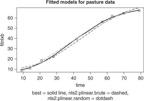
To visually compare the models found from each of the nls2 solutions above with the best solution found, we graph the fitted lines for all three models. So that we can compute the fitted values and graph them; we will use the wrapnls() function of nlmrt and graph the fits versus the original data (Figure 6.3). wrapnls() simply calls nls() with the results parameters of nlxb() to obtain the special result structure nls() offers. The residuals can also be displayed in boxplots to compare their sizes, and we present that display also (Figure 6.4).
require(nlmrt)
## Loading required package: nlmrt
splb <- coef(anls2plb)
splr <- coef(anls2plr)
names(splb) <- names(huetstart)
names(splr) <- names(huetstart)
anlsfromplb <- nls(regmod, start = splb, trace = FALSE, data = pastured)
anlsfromplr <- nls(regmod, start = splr, trace = FALSE, data = pastured)
agomp <- wrapnls(regmodf, start = huetstart, data = pastured)
fitnlxb <- fitted(agomp)
fitnls2b <- fitted(anls2plb)
fitnls2r <- fitted(anls2plr)
plot(pastured$time, fitnlxb, type = "l", lwd = 2, xlab = "time")
points(pastured$time, fitnls2b, col = "red", type = "l", lty = "dashed",
    lwd = 2)
points(pastured$time, fitnls2r, col = "blue", type = "l", lty = "dotdash",
    lwd = 2)
points(pastured$time, pastured$yield)
title(main = "Fitted models for pasture data")
sstr <- "best = solid line, nls2.plinear.brute = dashed, nls2.plinear.random = dotdash"
title(sub = sstr, cex.sub = 0.8)
resnlxb <- pastured$yield - fitnlxb
resnls2b <- pastured$yield - fitnls2b
resnls2r <- pastured$yield - fitnls2r
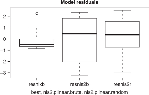
While the graphs show the nlxb() solution is “better” than the others, there remains a sense of discomfort that a reasonable solution has not been reliably obtained. Other experiments show that nlxb() can give unsatisfactory solutions from many sets of starting values. We were lucky here. Note that nls2() must be provided with intervals that include “good” parameters, thereby requiring us to have an idea where these are.
A similar variation in results is found by using the nlmrt codes model2ssfun() and model2grfun() to generate an objective function and its gradient for use with optimization routines.
ssfn <- model2ssfun(regmodf, ones)
grfn <- model2grfun(regmodf, ones)
time <- pastured$time
yield <- pastured$yield
# aopto<-optim(ones, ssfn, gr=grfn, yield=yield, time=time,
# method='BFGS', control=list(maxit=10000)) print(aopto) ##
# We did not run this one.
aopth <- optim(huetstart, ssfn, gr = grfn, yield = yield, time = time,
    method = "BFGS", control = list(maxit = 10000))
print(aopth)
## $par
##      t3      t4      t1      t2
## -9.2089  2.3778 69.9552 61.6815
##
## $value
## [1] 8.3759
##
## $counts
## function gradient
##       92       36
##
## $convergence
## [1] 0
##
## $message
## NULL
The conclusion of all this? While we can find acceptable solutions, the tools may not automatically provide us the evidence that we have the BEST solution. This is an area that is still worthy of research (into the mathematics) and development (of the software tools).
6.3 The structure of the nls() solution
The R function str() can quickly reveal what is returned by nls(), and it is an impressive set of capabilities. As indicated, my only concern is that it is too rich for many applications and users. Some users will also find that the nomenclature is at odds with usage in the optimization community. Suppose the solutions to the weight loss problem in Section 6.1.1 from nls() and nlxb() are wlnls and wlnlxb, respectively. The Jacobian of the residuals at the solution is obtained from wlnls as wlnls$m$gradient() (note that it is a function call), while from wlnlxb as wlnlxb$jacobian. This use of the term “gradient” carries over to the error message “singular gradient,” which, I believe, confuses users.
require(nlmrt)
wlmod <- "Weight ∼ b0 + b1*2^(-Days/th)"
wlnlxb <- nlxb(wlmod, data = wl, start = c(b0 = 1, b1 = 1, th = 1))
wlnlxb
## nlmrt class object: x
## residual sumsquares =  39.245  on  52 observations
##     after  9    Jacobian and  13 function evaluations
##   name       coeff       SE      tstat     pval      gradient    JSingval
## b0          81.3751      2.266      35.9         0   7.707e-05        8.53
## b1          102.683       2.08     49.36         0  -8.111e-05       1.427
## th          141.908      5.289     26.83         0  -2.634e-05      0.1471
Both nlxb() and nls() can use a function coef() to get at the parameters or coefficients of the linear model. Thus,
coef(wlnls)
##      b0      b1      th
##  81.374 102.684 141.910
coef(wlnlxb)
However, internally, nlxb() returns the coefficients as wlnlxb$coefficients, that is, as a simple element of the solution. By contrast, one needs to extract them from the nls() solution object using wlnls$m$getPars(). This is a function that appears to be undocumented by the conventional R approach of using ?getPars or ??getPars. It is visible by str(wlnls). There is also documentation in a web page titled “Create an nlsModel Object” at http://web.njit.edu/all_topics/Prog_Lang_Docs/html/library/nls/html/nlsModel.html. However, I could not find this page in the main R manuals on the www.r-project.org web site. My complaint is not that the information is at all difficult to obtain once the mechanism is known but that finding how to do so requires more digging than it should.
Certainly, as I point out in the Chapter 3, it is difficult to structure the output of complicated tools like nls() in a manner that is universally convenient. Knowing how to use functions getPars() or coef(wlnls), users can quickly access the information they need. There is yet another possibility in summary(wlnls)$coefficients[,1].
It is helpful to be able to extract a set of parameters (coefficients) from one solution or model and try it in another solver as a crude check for stability of these estimates or, as in the control parameter follow.on in package optimx, to be able to run an abbreviated solution process with one solver to get close to a solution and then use another to complete the process. This approach tries to take advantage of differential advantages of different methods.
Unlike nls() or nlsLM of minpack.lm, nlmrt tools generally do not return the large nls-style object. In part, this is not only because the nlmrt tools are intended to deal with the zero-residual case where some of the parts of the nlsModel structure make little sense but also because I prefer a simpler output object. However, as mentioned, there is wrapnls that calls nls() appropriately (i.e., with bounds) after running nlxb().
6.4 Concerns with nls()
nls() seems to be designed mainly for nonlinear regression, so it is not entirely suitable for general nonlinear least squares computations. In my view, the following are the main issues, which are sometimes seen in similar codes both in R and other systems.
- It is specifically NOT indicated for problems where the residuals are small or zero. Thus it excludes many approximation problems.
- It frequently fails to find a solution to problems that other methods solve easily, giving a cryptic “singular gradient” error message.
- Bounds on parameters require the use of the “port” algorithm. Unless this is specified, bounds are ignored.
- Because the solution object from
nls()is complicated, extracting information from it can be error prone. Some of this output (e.g., “achieved convergence tolerance”) is not fully explained.
6.4.1 Small residuals
The nls() manual is specific in warning that it should not be used for problems with “artificial ‘zero-residual’ data.” In such cases, the manual suggests adding some noise to the data. As we have seen, nonlinear equations problems give rise to zero-residual nonlinear least squares problems, as do certain approximation and interpolation problems, where adding noise destroys the value of the solutions. The restriction with nls() arises because of software design choices rather than fundamental algorithmic reasons. While the implementation choices for nls() may be sensible in the context of traditional statistical estimation, they are unhelpful to general users.
In fact, the nonlinear least squares problem is generally well defined when the residuals are small or zero. The difficulty for nls() comes not from the Gauss–Newton method, but rather the particular relative offset convergence test (Bates and Watts, 1981). This tries to compare the change in parameters to a measure that is related to the size of the residuals, essentially dividing zero by zero. In an appropriate context, the Bates–Watts convergence test is a “very good idea,” and I decided to incorporate a version of this test in nlmrt while writing this section. However, far from all nonlinear least squares problems fit its assumptions. I am, in fact, surprised nls() does not appear to offer a way to simply select a more mundane convergence test.
Packages nlmrt and minpack.lm have ways to select suitable termination criteria when the residuals are very small. In nlmrt, the functions nlxb() and nlfb() allow the control list elements rofftest and smallsstest to be set FALSE. The first choice turns off the relative offset test, thereby trying harder to find a minimum. The second choice ignores a test of the size of the sum of squares. If we expect our residuals to be somewhere in the scale of 1 to 10, a very small sum of squares would imply we are finished, and keeping the default test for a small sum of squares makes sense. For problems where our fit could be exact, we should turn off this termination condition.
x <- 1:10
y <- 2 * x + 3  # perfect fit
yeps <- y + rnorm(length(y), sd = 0.01)  # added noise
anoise <- nls(yeps ∼ a + b * x, start = list(a = 0.12345, b = 0.54321))
summary(anoise)
##
## Formula: yeps ∼ a + b * x
##
## Parameters:
##   Estimate Std. Error t value Pr(>|t|)
## a  3.01098    0.00699     431   <2e-16 ***
## b  1.99857    0.00113    1775   <2e-16 ***
## - - -
## Signif. codes:  0 '***' 0.001 '**' 0.01 '*' 0.05 '.' 0.1 ' ' 1
##
## Residual standard error: 0.0102 on 8 degrees of freedom
##
## Number of iterations to convergence: 2
## Achieved convergence tolerance: 3.91e-09
aperf <- try(nls(y ∼ a + b * x, start = list(a = 0.12345, b = 0.54321)))
print(strwrap(aperf))
## [1] "Error in nls(y ∼ a + b * x, start = list(a = 0.12345,"
## [2] "b = 0.54321)) : number of iterations exceeded maximum"
## [3] "of 50"
ldata <- data.frame(x = x, y = y)
aperfn <- try(nlxb(y ∼ a + b * x, start = list(a = 0.12345, b = 0.54321),
    data = ldata))
aperfn
## nlmrt class object: x
## residual sumsquares =  4.5342e-20  on  10 observations
##     after  3    Jacobian and  4 function evaluations
##   name       coeff        SE       tstat    pval      gradient    JSingval
## a                 3   5.143e-11  5.833e+10        0   1.671e-10       19.82
## b                 2   8.289e-12  2.413e+11        0  -9.542e-10       1.449
6.4.2 Robustness—“singular gradient” woes
We have already seen an example of nls() stopping with the “singular gradient” termination message. While Marquardt approaches may also fail, they are generally more robust than the Gauss–Newton method of nls().
The following problem was posted on the Rhelp list. It has only four observations to try to fit three parameters, so we may fully expect strange results. The first try results in the common “singular gradient” error with nls(), but nlxb() can find a solution.
x <- c(60, 80, 100, 120)
y <- c(0.8, 6.5, 20.5, 45.9)
mydata <- data.frame(x, y)
pnames <- c("a", "b", "d")
npar <- length(pnames)
st <- c(1, 1, 1)
names(st) <- pnames
rnls <- try(nls(y ∼ exp(a + b * x) + d, start = st, data = mydata),
    silent = TRUE)
if (class(rnls) == "try-error") {
    cat("nls() failed (singular gradient?)
")
} else {
    summary(rnls)
}
## nls() failed (singular gradient?)
require(nlmrt)
rnlx0 <- try(nlxb(y ∼ exp(a + b * x) + d, start = st, data = mydata),
    silent = TRUE)
cat("Found sum of squares ", rnlx0$ssquares, "
")
## Found sum of squares  1.701e+104
print(rnlx0$coefficients)
##           a           b           d
##  5.0003e-01  9.9583e-01 -5.9072e+47
## Now turn off relative offset test
rnlx1 <- try(nlxb(y ∼ exp(a + b * x) + d, start = st, data = mydata,
    control = list(rofftest = FALSE)), silent = TRUE)
cat("Found sum of squares ", rnlx1$ssquares, "
")
## Found sum of squares  2.3892e+50
coef(rnlx1)
## And the sumsquares size test
rnlx2 <- try(nlxb(y ∼ exp(a + b * x) + d, start = st, data = mydata,
    control = list(rofftest = FALSE, smallsstest = FALSE)), silent = TRUE)
cat("Found sum of squares ", rnlx2$ssquares, "
")
## Found sum of squares  0.57429
coef(rnlx2)
Note how wild the results are unless we are very aggressive in keeping the algorithm working by turning off relative offset and “small” sumsquares tests. In this case, “small” is (100∗.Machine$double.eps)∧4 = 2.430865e![]() 55 times the initial sum of squares (of the order of 1e
55 times the initial sum of squares (of the order of 1e![]() 105), which is still bigger than 1e
105), which is still bigger than 1e![]() 50. This is a very extreme problem, although it looks quite ordinary.
50. This is a very extreme problem, although it looks quite ordinary.
To explore the possibility that different starting values for the parameters might be important for success, we will generate 1000 sets of starting parameters in a box from 0 to 8 on each edge using uniformly distributed pseudorandom numbers. Then we will try to solve the problem just presented from these starting points with nls() and nlxb() (from nlmrt). We will not show the code here, which is simple but a bit tedious. Note that the nlxb() is called with the control elements rofftest=FALSE and smallsstest=FALSE. Besides actual failures to terminate normally, we judge any solution with a sum of squares exceeding 0.6 as failures.
## Proportion of nls  runs that failed =  0.728
## Proportion of nlxb runs that failed =  0
## Average iterations for nls = 20.018
## Average jacobians for nlxb = 66.684
## Average residuals for nlxb = 80.463
This is just one numerical experiment—a very extreme one—and we should be cautious about the lessons we take from it. However, it does mirror my experiences, namely,
- the Marquardt approach is generally much more successful in finding solutions than the Gauss–Newton approach that
nls()uses; - a relative offset test of the type always used in
nls()but which can be ignored innlxb()is not appropriate for extreme problems; - when they do find solutions, Gauss–Newton methods like
nls()are generally more efficient than Marquardt methods.
6.4.3 Bounds with nls()
My concerns here are best summarized by quoting two portions of the nls() manual:
   Bounds can only be used with the "port" algorithm.
   They are ignored, with a warning, if given for other algorithms.
    The 'algorithm = "port"' code appears unfinished, and does not
     even check that the starting value is within the bounds.  Use with
     caution, especially where bounds are supplied.
In fact, I have NOT found any issues with using the “port” code. I am more concerned that bounds are ignored, although a warning is issued. I would rather that the program stop in this case, as users are inclined to ignore warnings.
The nlxb() function handles bounds and seems to work properly. I have found (and reported to the maintainers) that nlsLM() can sometimes stop too soon. I believe this is due to a failure to project the Marquardt search direction onto the feasible hyperplane, which requires action inside the Marquardt code. In actuality, one needs to check if the search will or will not bump into the bound and either free or impose the constraint. In the case of package minpack.lm, the program code where this must happen is inside non-R code that is messy to adjust.
Using the scaled Hobbs problem of Section 1.2, let us try simple upper bounds at 2 on all parameters and apply nls(), nlxb(), and nlsLM(). We need to ensure that we consider the sum of squares, which shows the last one has stopped prematurely.
ydat <- c(5.308, 7.24, 9.638, 12.866, 17.069, 23.192, 31.443,
    38.558, 50.156, 62.948, 75.995, 91.972)  # for testing
tdat <- 1:length(ydat)  # for testing
weeddata <- data.frame(y = ydat, t = tdat)
require(nlmrt)
require(minpack.lm)
hobmod <- "y∼100*b1/(1+10*b2*exp(-0.1*b3*t))"
st <- c(b1 = 1, b2 = 1, b3 = 1)
low <- c(-Inf, -Inf, -Inf)
up <- c(2, 2, 2)
cat("try nlxb
")
## try nlxb
anlxb2 <- nlxb(hobmod, st, data = weeddata, lower = low, upper = up)
anlxb2
## nlmrt class object: x
## residual sumsquares =  839.73  on  12 observations
##     after  7    Jacobian and  8 function evaluations
##   name       coeff       SE      tstat     pval      gradient    JSingval
## b1                2U        NA        NA        NA           0       60.46
## b2          1.78636         NA        NA        NA  -3.637e-05           0
## b3                2U        NA        NA        NA           0           0
try(anls2p <- nls(hobmod, st, data = weeddata, lower = low, upper = up,
    algorithm = "port"))
summary(anls2p)
##
## Formula: y ∼ 100 * b1/(1 + 10 * b2 * exp(-0.1 * b3 * t))
##
## Parameters:
##    Estimate Std. Error t value Pr(>|t|)
## b1     2.00       3.96    0.50     0.63
## b2     1.79       3.08    0.58     0.58
## b3     2.00       1.21    1.66     0.13
##
## Residual standard error: 9.66 on 9 degrees of freedom
##
## Algorithm "port", convergence message: relative convergence (4)
anls2p$m$deviance()
## [1] 839.73
aLM2 <- nlsLM(hobmod, st, data = weeddata, lower = low, upper = up)
summary(aLM2)
##
## Formula: y ∼ 100 * b1/(1 + 10 * b2 * exp(-0.1 * b3 * t))
##
## Parameters:
##    Estimate Std. Error t value Pr(>|t|)
## b1     2.00       5.12    0.39     0.71
## b2     2.00       4.49    0.44     0.67
## b3     2.00       1.41    1.42     0.19
##
## Residual standard error: 10.5 on 9 degrees of freedom
##
## Number of iterations to convergence: 2
## Achieved convergence tolerance: 1.49e-08
aLM2$m$deviance()
## [1] 987.58
6.5 Some ancillary tools for nonlinear least squares
Because of the importance and generality of nonlinear least squares problems, there are many add-on tools. We consider only some of them here.
6.5.1 Starting values and self-starting problems
Note that all of the methods we discuss assume that the user has in some way provided some data, and most approaches also ask for some preliminary guesses for the values of the parameters (coefficients) of the model.
nlxb() always requires a start vector of parameters. nls() includes a provision to try 1 for all parameters as a start if none is provided. While I have considered making the change to nlxb() to do this and often use such a starting vector myself, I believe it should be a conscious choice. Therefore, I am loath to provide such a default.
Good starting vectors really do help to save effort and get better solutions. For nls(), there are a number of self-starting models. In particular, the SSlogis model provides a form of the three-parameter logistic that we used to model the Hobbs data earlier. We explore this reparameterization in Chapter 16, and the details of the model are there, but it is useful to show how to use the tool that is in R.
## Put in weeddata here as precaution. Maybe reset workspace.
anlss2 <- nls(y ∼ SSlogis(t, p1, p2, p3), data = weeddata)
summary(anlss2)
##
## Formula: y ∼ SSlogis(t, p1, p2, p3)
##
## Parameters:
##    Estimate Std. Error t value Pr(>|t|)
## p1 196.1863    11.3069    17.4  3.2e-08 ***
## p2  12.4173     0.3346    37.1  3.7e-11 ***
## p3   3.1891     0.0698    45.7  5.8e-12 ***
## - - -
## Signif. codes:  0 '***' 0.001 '**' 0.01 '*' 0.05 '.' 0.1 ' ' 1
##
## Residual standard error: 0.536 on 9 degrees of freedom
##
## Number of iterations to convergence: 0
## Achieved convergence tolerance: 2.13e-07
anlss2$m$deviance()
## [1] 2.587
Note that the sum of squared residuals is the square of the residual standard error times the degrees of freedom. We can also use the deviance() supplied in the solution object.
6.5.2 Converting model expressions to sum-of-squares functions
Sometimes we want to use an R function to compute the residuals, Jacobian, or the sum-of-squares function so we can use optimization tools like those in optim(). See Section 6.6. So far, we have looked at tools that express the problem in terms of a model expression.
We can, of course, write such functions manually, but package nlmrt and some others offer tools to do this, such as four tools that start with
model2ssfun(): to create a sum of squares function;model2resfun(): to create a function that computes the residuals;model2jacfun(): to create a function that computes the Jacobian;model2grfun(): to create a function that computes the gradient.
These functions require the formula as well as a “typical” starting vector (to provide the names of the parameters).
There are also two tools that work with the residual and Jacobian functions and compute the sum of squares and gradient from them.
modss(): to compute the sum of squares by computing the residuals and forming their cross-product;modgr(): to compute the gradient of the sum of squares from the residuals and the Jacobian.
These two functions require functions for the residuals and the Jacobian in their calling syntax.
6.5.3 Help for nonlinear regression
This book is mostly about the engines inside the vehicles for nonlinear optimization, but many people are more concerned with the bodywork and passenger features of the nonlinear modeling cars. Fortunately, there are some useful reference works on this topic, and some are directed at R users. In particular, Ritz and Streibig (2008) is helpful. There are also some good examples in Huet et al. (1996), but the software used is not mainstream to R. Older books have a lot of useful material, but their ideas must be translated to the R context. Among these are Bates and Watts (1988), Seber and Wild (1989), Nash and Walker-Smith (1987), Ratkowsky (1983), and Ross (1990).
6.6 Minimizing R functions that compute sums of squares
Package nlmrt and package minpack.lm include tools to minimize sums-of-squares residuals expressed as functions rather than expressions. They both use Marquardt-based methods to solve nonlinear least squares problems. We have already seen nlxb() and nlsLM(). However, both nls.lm from minpack.lm and nlfb from nlmrt are designed to work with a function to compute the vector of residuals at a given set of parameters, with (optionally) a function to compute the Jacobian matrix.
## weighted nonlinear regression
Treated <- as.data.frame(Puromycin[Puromycin$state == "treated",
    ])
weighted.MM <- function(resp, conc, Vm, K) {
    ## Purpose: exactly as white book p. 451 -- RHS for nls()
    ## Weighted version of Michaelis-Menten model
    ## - - - - - - - - - - - - - - - - - - - - - - - - - - - - - - - - - - - - - - - - - - - - - - - - - - - - - - -
    ## Arguments: 'y', 'x' and the two parameters (see book)
    ## - - - - - - - - - - - - - - - - - - - - - - - - - - - - - - - - - - - - - - - - - - - - - - - - - - - - - - -
    ## Author: Martin Maechler, Date: 23 Mar 2001
    pred <- (Vm * conc)/(K + conc)
    (resp - pred)/sqrt(pred)
}
wtMM <- function(x, resp, conc) {
    # redefined for nlfb()
    Vm <- x[1]
    K <- x[2]
    res <- weighted.MM(resp, conc, Vm, K)
}
start <- list(Vm = 200, K = 0.1)
Pur.wt <- nls(∼weighted.MM(rate, conc, Vm, K), data = Treated,
    start)
print(summary(Pur.wt))
##
## Formula: 0 ∼ weighted.MM(rate, conc, Vm, K)
##
## Parameters:
##    Estimate Std. Error t value Pr(>|t|)
## Vm 2.07e+02   9.22e+00   22.42  7.0e-10 ***
## K  5.46e-02   7.98e-03    6.84  4.5e-05 ***
## - - -
## Signif. codes:  0 '***' 0.001 '**' 0.01 '*' 0.05 '.' 0.1 ' ' 1
##
## Residual standard error: 1.21 on 10 degrees of freedom
##
## Number of iterations to convergence: 5
## Achieved convergence tolerance: 3.83e-06
require(nlmrt)
anlf <- nlfb(start, resfn = wtMM, jacfn = NULL, trace = FALSE,
    conc = Treated$conc, resp = Treated$rate)
anlf
## nlmrt class object: x
## residual sumsquares =  14.597  on  12 observations
##     after  6    Jacobian and  7 function evaluations
##   name      coeff        SE      tstat      pval      gradient   JSingval
## Vm         206.835       9.225     22.42  7.003e-10  -9.708e-11      230.7
## K        0.0546112    0.007979     6.845  4.488e-05  -7.255e-09      0.131
6.7 Choosing an approach
We have seen that solving nonlinear least squares problems with R generally takes one of two approaches, either via a modeling expression or one or more functions that compute the residuals and related quantities. These approaches have a quite different “feel.” When we work with residual functions, we will often think of their derivatives—the Jacobian—whereas expression-based tools attempt to generate such information. In that task, nls() has more features than nlxb(), as we shall see in the following example. By contrast, we generally have a lot more flexibility in defining the residuals when taking a function approach.
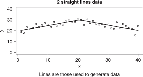
The problem we shall use to illustrate the differences in approach will be referred to as the “two straight line” problem. Here we want to model data using two straight line models that intersect at some point (Figure 6.5). This problem was of interest to a colleague at Agriculture Canada in the 1970s. See Nash and Price (1979). For the present example, we will generate some data.
set.seed(1235)
x <- 1:40
xint <- 20.5 * rep(1, length(x))
sla <- 0.5
slb <- -0.5
yint <- 30
idx <- which(x <= xint)
ymod <- {
    yint + (x - xint) * slb
}
ymod[idx] <- yint + (x[idx] - xint[idx]) * sla
ydata <- ymod + rnorm(length(x), 0, 2)
plot(x, ymod, type = "l", ylim = c(0, 40), ylab = "y")
points(x, ydata)
title(main = "2 straight lines data")
title(sub = "Lines are those used to generate data")
We can model this data quite nicely with nls() if we take a little care in how we define the modeling expression and select starting values. Note that we are supposed to be able to leave out start, but that does not seem to work here. Nor does putting in a very naive set of starting parameters. However, a very rough choice does work.
tslexp <- "y ∼ (yint + (x-xint)*slb)*(x>= xint) + (yint + (x-xint)*sla)*( x < xint)"
mydf <- data.frame(x = x, y = ydata)
mnls <- try(nls(tslexp, trace = FALSE, data = mydf))
strwrap(mnls)
## [1] "Error in getInitial.default(func, data, mCall ="
## [2] "as.list(match.call(func, : no 'getInitial' method"
## [3] "found for "function" objects"
mystart <- c(xint = 1, yint = 1, sla = 1, slb = 1)
mnls <- try(nls(tslexp, start = mystart, trace = FALSE, data = mydf))
strwrap(mnls)
## [1] "Error in nlsModel(formula, mf, start, wts) : singular"
## [2] "gradient matrix at initial parameter estimates"
myst2 <- c(xint = 15, yint = 25, sla = 1, slb = -1)
mnls2 <- try(nls(tslexp, start = myst2, trace = FALSE, data = mydf))
summary(mnls2)
##
## Formula: y ∼ (yint + (x - xint) * slb) * (x >= xint) + (yint + (x - xint) *
##     sla) * (x < xint)
##
## Parameters:
##      Estimate Std. Error t value Pr(>|t|)
## xint  19.9341     1.5623   12.76  6.4e-15 ***
## yint  29.4904     0.6922   42.61  < 2e-16 ***
## sla    0.4617     0.0915    5.05  1.3e-05 ***
## slb   -0.4276     0.0787   -5.43  4.0e-06 ***
## - - -
## Signif. codes:  0 '***' 0.001 '**' 0.01 '*' 0.05 '.' 0.1 ' ' 1
##
## Residual standard error: 2.18 on 36 degrees of freedom
##
## Number of iterations to convergence: 5
## Achieved convergence tolerance: 8.05e-09
mnls2$m$deviance()
## [1] 171.62
Unfortunately, as yet nlxb() does not handle this model form.
require(nlmrt)
mnlxb <- try(nlxb(tslexp, start = mystart, trace = FALSE, data = mydf))
strwrap(mnlxb)
## [1] "Error in deriv.default(parse(text = resexp),"
## [2] "names(start)) : Function ''<'' is not in the"
## [3] "derivatives table"
By the time this book is published, this obstacle may be overcome. However, in the meantime, it is relatively straightforward to convert the problem to one involving a residual function and to call nlfb() using a numerical Jacobian approximation.
myres <- model2resfun(tslexp, mystart)
## Now check the calculation
tres <- myres(myst2, x = mydf$x, y = mydf$y)
tres
##  [1]  -7.85402  -6.18029 -10.22992  -7.97355  -7.47842
##  [6] -10.14639  -6.34569  -7.05972  -7.98057  -5.55515
## [11]  -2.36927  -5.91993  -1.74969  -1.90661  -0.60365
## [16]  -4.57540  -6.47660  -5.84212  -6.91754 -10.38309
## [21] -10.74823  -7.26064 -14.16750 -11.29679 -13.85938
## [26] -12.55585 -12.68729 -14.22140 -12.35207 -15.71322
## [31] -13.14478 -13.50182 -21.21353 -16.25285 -21.17923
## [36] -20.28866 -19.61445 -19.45144 -14.75980 -24.25293
## But jacobian fails
jactry <- try(myjac <- model2jacfun(tslexp, mystart))
strwrap(jactry)
## [1] "Error in deriv.default(parse(text = resexp), pnames)"
## [2] ": Function ''<'' is not in the derivatives table"
## Try nlfb with no jacfn.
mnlfb <- try(nlfb(mystart, resfn = myres, trace = FALSE, x = mydf$x,
    y = mydf$y))
mnlfb
## nlmrt class object: x
## residual sumsquares =  434.73  on  40 observations
##     after  4    Jacobian and  5 function evaluations
##   name       coeff       SE      tstat     pval      gradient    JSingval
## xint       -10.4204         NA        NA        NA   9.993e-09       208.8
## yint        25.1081         NA        NA        NA   7.067e-10       2.211
## sla               1         NA        NA        NA           0    7.68e-09
## slb     -0.00182172         NA        NA        NA   3.604e-08   5.527e-23
## Also try from better start
mnlfb2 <- try(nlfb(myst2, resfn = myres, trace = FALSE, x = mydf$x,
    y = mydf$y))
mnlfb2
## nlmrt class object: x
## residual sumsquares =  171.62  on  40 observations
##     after  6    Jacobian and  7 function evaluations
##   name       coeff        SE      tstat      pval      gradient   JSingval
## xint        19.9341       1.562     12.76  6.217e-15  -2.978e-13         54
## yint        29.4904      0.6922     42.61          0   6.917e-12      49.62
## sla        0.461741     0.09145     5.049  1.294e-05   3.462e-11      3.148
## slb       -0.427626     0.07868    -5.435   3.96e-06  -3.232e-11      1.395
## It will also work with mnlfb2j<-try(nlfb(myst2,
## resfn=myres, jacfn=NULL, trace=FALSE, x=mydf$x, y=mydf$y))
## or with Package pracma's function lsqnonlin (but there is
## not a good summary())
require(pracma)
alsqn <- lsqnonlin(myres, x0 = myst2, x = mydf$x, y = mydf$y)
print(alsqn$ssq)
## [1] 171.62
print(alsqn$x)
##     xint     yint      sla      slb
## 19.93411 29.49038  0.46174 -0.42763
We can also show that minpack.lm can use either its expression-based nlsLM() or function-based nls.lm() to solve this problem.
It is also possible to think of the problem as a one-dimensional minimization, where we choose an ![]() -value for the intersection of the two lines and compute separate linear models to the left and right of this divider, with the objective function the sum of the two sums of squares. The glitch in this approach (which “mostly” works) is that sometimes the two lines do not intersect near the chosen
-value for the intersection of the two lines and compute separate linear models to the left and right of this divider, with the objective function the sum of the two sums of squares. The glitch in this approach (which “mostly” works) is that sometimes the two lines do not intersect near the chosen ![]() -value. In such cases, the apparent sum of squares is too low.
-value. In such cases, the apparent sum of squares is too low.
This problem is one of many where a relatively simple change to a linear modeling task gives rise to a problem that is in some ways nonlinear. Many constrained linear model problems, such as nonnegative least squares, the present two or more straight lines problem, and the Hassan problem from Nash (1979, p. 184) that is treated in Chapter 13 can all be approached using nonlinear least squares tools.
6.8 Separable sums of squares problems
In many situations, we encounter problems where we need to solve a nonlinear least squares problem but the model to be fitted has several linear parameters, or else can be thus reorganized. We already encountered this in the Pasture problem earlier. A classic example is the multiple exponentials model that occurs when we have, for example, the radioactive decay over time of a mixture of two radioactive elements with different half-lives. The measured radioactivity ![]() is the sum of the radiation from each and will decay over time, which is given the variable
is the sum of the radiation from each and will decay over time, which is given the variable ![]() here.
here.
where ![]() and
and ![]() are the amounts or concentrations of each of the elements and the
are the amounts or concentrations of each of the elements and the ![]() and
and ![]() are their decay rates.
are their decay rates.
In practice, it is fairly easy to get a good “fit” to the data, but if we artificially generate data from a particular example of such a model, it is exceedingly difficult to recover the input parameters. There are often many parameter sets that fit the data equally well. This has been well known for a long time, and we will use a classic example from Lanczos (1956, p. 276). This is two-decimal data for 24 values of the ![]() data generated from a sum of three exponentials.
data generated from a sum of three exponentials.
require(NISTnls)
L1 <- Lanczos1  # The data frame of data, but more than 2 decimals on y
L1[, "y"] <- round(L1[, "y"], 2)
L1
##       y    x
## 1  2.51 0.00
## 2  2.04 0.05
## 3  1.67 0.10
## 4  1.37 0.15
## 5  1.12 0.20
## 6  0.93 0.25
## 7  0.77 0.30
## 8  0.64 0.35
## 9  0.53 0.40
## 10 0.45 0.45
## 11 0.38 0.50
## 12 0.32 0.55
## 13 0.27 0.60
## 14 0.23 0.65
## 15 0.20 0.70
## 16 0.17 0.75
## 17 0.15 0.80
## 18 0.13 0.85
## 19 0.11 0.90
## 20 0.10 0.95
## 21 0.09 1.00
## 22 0.08 1.05
## 23 0.07 1.10
## 24 0.06 1.15
It is straightforward to write down a function for the residuals (here in “model-data” form). The Jacobian function is also straightforward. We also set some starting vectors, for which parameter names are provided. This is not strictly necessary for a function approach to the problem but is required for the expression approach of nls(). We write the model expression at the end of the code segment.
lanc.res <- function(b, data) {
    # 3 exponentials
    res <- rep(NA, length(data$x))
    res <- b[4] * exp(-b[1] * data$x) + b[5] * exp(-b[2] * data$x) +
        b[6] * exp(-b[3] * data$x) - data$y
}
lanc.jac <- function(b, data) {
    # 3 exponentials
    expr3 <- exp(-b[1] * data$x)
    expr7 <- exp(-b[2] * data$x)
    expr12 <- exp(-b[3] * data$x)
    J <- matrix(0, nrow = length(data$x), ncol = length(b))
    J[, 4] <- expr3
    J[, 1] <- -(b[4] * (expr3 * data$x))
    J[, 5] <- expr7
    J[, 2] <- -(b[5] * (expr7 * data$x))
    J[, 6] <- expr12
    J[, 3] <- -(b[6] * (expr12 * data$x))
    J
}
bb1 <- c(1, 2, 3, 4, 5, 6)
bb2 <- c(1, 1.1, 1.2, 0.1, 0.1, 0.1)
names(bb1) <- c("a1", "a2", "a3", "c1", "c2", "c3")
names(bb2) <- c("a1", "a2", "a3", "c1", "c2", "c3")
## Check residual function
cat("Sumsquares at bb1 =", as.numeric(crossprod(lanc.res(bb1,
    data = L1))))
## Sumsquares at bb1 = 966.43
require(numDeriv)
JJ <- lanc.jac(bb1, data = L1)
JJn <- jacobian(lanc.res, bb1, data = L1)
cat("max abs deviation JJ and JJn:", max(abs(JJ - JJn)), "
")
## max abs deviation JJ and JJn: 2.5033e-10
lancexp <- "y ∼ (c1*exp(-a1*x) + c2*exp(-a2*x) + c3*exp(-a3*x))"
Note that we test the functions. I recommend this be done in EVERY case. In the present example, the tests caught an error in lanc.res() where I had the final “+” sign at the beginning of the last line rather than at the end of the penultimate line. A seemingly trivial but important mistake.
Let us now test several different approaches to the problem using both starting vectors.
tnls1 <- try(nls(lancexp, start = bb1, data = Lanczos1, trace = FALSE))
strwrap(tnls1)
## [1] "Error in numericDeriv(form[[3L]], names(ind), env) :"
## [2] "Missing value or an infinity produced when evaluating"
## [3] "the model"
tnls2 <- try(nls(lancexp, start = bb2, data = Lanczos1, trace = FALSE))
strwrap(tnls2)
## [1] "Error in nlsModel(formula, mf, start, wts) : singular"
## [2] "gradient matrix at initial parameter estimates"
## nlmrt
require(nlmrt)
tnlxb1 <- try(nlxb(lancexp, start = bb1, data = Lanczos1, trace = FALSE))
tnlxb1
## nlmrt class object: x
## residual sumsquares =  5.3038e-09  on  24 observations
##     after  9    Jacobian and  10 function evaluations
##   name      coeff       SE     tstat      pval      gradient    JSingval
## a1        0.887574    0.06331    14.02  3.976e-11   -3.23e-06        4.02
## a2         2.87509    0.05719    50.27          0  -1.765e-05       1.162
## a3         4.96068    0.01666    297.8          0  -1.866e-05      0.2251
## c1       0.0752577    0.00897     8.39  1.236e-07   0.0001546     0.03114
## c2         0.81353    0.01928    42.19          0   9.004e-05    0.002182
## c3          1.6246    0.02808    57.86          0   5.637e-05   0.0001837
tnlxb2 <- try(nlxb(lancexp, start = bb2, data = Lanczos1, trace = FALSE))
tnlxb2
## nlmrt class object: x
## residual sumsquares =  4.2906e-06  on  24 observations
##     after  42    Jacobian and  57 function evaluations
##   name       coeff       SE      tstat     pval      gradient    JSingval
## a1          1.87271         NA        NA        NA   4.242e-08       6.007
## a2          1.87274         NA        NA        NA  -3.419e-08        2.57
## a3          4.63965         NA        NA        NA    2.42e-09      0.2743
## c1          4.99146         NA        NA        NA  -1.174e-08     0.02612
## c2         -4.54744         NA        NA        NA  -1.174e-08    1.59e-06
## c3          2.06878         NA        NA        NA  -2.199e-09   1.887e-16
tnlfb1 <- try(nlfb(bb1, lanc.res, trace = FALSE, data = Lanczos1))
tnlfb1
## nlmrt class object: x
## residual sumsquares =  5.3036e-09  on  24 observations
##     after  9    Jacobian and  10 function evaluations
##   name       coeff       SE     tstat      pval      gradient    JSingval
## a1         0.887576    0.06331    14.02  3.974e-11   -3.23e-06        4.02
## a2          2.87509    0.05719    50.28          0  -1.765e-05       1.162
## a3          4.96068    0.01666    297.8          0  -1.866e-05      0.2251
## c1        0.0752581    0.00897     8.39  1.235e-07   0.0001546     0.03114
## c2         0.813531    0.01928    42.19          0   9.004e-05    0.002182
## c3           1.6246    0.02808    57.86          0   5.637e-05   0.0001837
tnlfb2 <- try(nlfb(bb2, lanc.res, trace = FALSE, data = Lanczos1))
tnlfb2
## nlmrt class object: x
## residual sumsquares =  4.2906e-06  on  24 observations
##     after  42    Jacobian and  57 function evaluations
##   name      coeff       SE       tstat      pval      gradient    JSingval
## a1         1.87271      220.7   0.008486     0.9933    4.24e-08       6.007
## a2         1.87274      240.8   0.007776     0.9939  -3.418e-08        2.57
## a3         4.63965    0.06845      67.79          0    2.42e-09      0.2743
## c1         4.99147     346190  1.442e-05          1  -1.174e-08     0.02612
## c2        -4.54745     346190 -1.314e-05          1  -1.174e-08    1.59e-06
## c3         2.06878     0.1006      20.56  5.973e-14    -2.2e-09   9.972e-10
tnlfb1j <- try(nlfb(bb1, lanc.res, lanc.jac, trace = FALSE, data = Lanczos1))
tnlfb1j
## nlmrt class object: x
## residual sumsquares =  5.3038e-09  on  24 observations
##     after  9    Jacobian and  10 function evaluations
##   name      coeff       SE      tstat      pval      gradient    JSingval
## a1        0.887574    0.06331     14.02  3.976e-11   -3.23e-06        4.02
## a2         2.87509    0.05719     50.27          0  -1.765e-05       1.162
## a3         4.96068    0.01666     297.8          0  -1.866e-05      0.2251
## c1       0.0752577    0.00897      8.39  1.236e-07   0.0001546     0.03114
## c2         0.81353    0.01928     42.19          0   9.004e-05    0.002182
## c3          1.6246    0.02808     57.86          0   5.637e-05   0.0001837
tnlfb2j <- try(nlfb(bb2, lanc.res, lanc.jac, trace = FALSE, data = Lanczos1))
tnlfb2j
## nlmrt class object: x
## residual sumsquares =  4.2906e-06  on  24 observations
##     after  42    Jacobian and  57 function evaluations
##   name       coeff        SE      tstat     pval      gradient    JSingval
## a1          1.87271          NA        NA        NA   4.242e-08       6.007
## a2          1.87274          NA        NA        NA  -3.419e-08        2.57
## a3          4.63965          NA        NA        NA    2.42e-09      0.2743
## c1          4.99146          NA        NA        NA  -1.174e-08     0.02612
## c2         -4.54744          NA        NA        NA  -1.174e-08    1.59e-06
## c3          2.06878          NA        NA        NA  -2.199e-09   2.942e-16
From the above, we see that it is quite difficult to recover the original exponential parameters (1, 3, and 5). This might be expected, as there is nothing to prevent the three exponential terms from switching roles during the sum-of-squares minimization. Indeed one of the proposed solutions has found what appears to be a saddle point with small gradient, singular Jacobian and two of the exponential parameters are the same. Note that the sum of squares is very small.
nls() should not, of course, be expected to deal with this small-residual problem. However, its “plinear” algorithm does quite well from the start bb1s except for the failure of the relative offset convergence test on the small residuals. The number of iterations has been limited to 20 to reduce output.
bb1s <- bb1[1:3]  # shorten start, as only 3 starting nonlinear parameters
bb2s <- bb2[1:3]
llexp <- "y∼cbind(exp(-a1*x), exp(-a2*x), exp(-a3*x))"
tnls1p <- try(nls(llexp, start = bb1s, data = Lanczos1, algorithm = "plinear",
    trace = TRUE, control = list(maxiter = 20)))
## 0.007251 :   1.0000  2.0000  3.0000  0.9718 -3.8894  5.3912
## 0.0006056 :   1.29580 -0.04136  4.79435  0.48291 -0.06102  2.10094
## 0.000102 :   2.466172 -0.989412  4.744276  0.667864  0.006105  1.835376
## 1.281e-07 :   2.257394 -0.788374  4.795171  0.620122  0.003522  1.889673
## 9.748e-08 :   2.295432 -0.514802  4.806250  0.633739  0.005439  1.874171
## 8.308e-08 :   2.336692 -0.275700  4.817737  0.647657  0.008083  1.857636
## 7.818e-08 :   2.38021 -0.07137  4.82939  0.66150  0.01150  1.84040
## 7.705e-08 :  2.42499 0.10063 4.84101 0.67502 0.01564 1.82276
## 7.596e-08 :  2.4701 0.2443 4.8525 0.6881 0.0204 1.8049
## 7.317e-08 :  2.51480 0.36385 4.86370 0.70065 0.02561 1.78717
## 6.834e-08 :  2.5584 0.4634 4.8746 0.7127 0.0311 1.7696
## 6.187e-08 :  2.60027 0.54639 4.88513 0.72436 0.03669 1.75239
## 5.444e-08 :  2.64003 0.61569 4.89522 0.73552 0.04221 1.73571
## 5.018e-08 :  2.71463 0.73165 4.91441 0.75636 0.05338 1.70369
## 4.808e-08 :  2.84063 0.88892 4.94806 0.79338 0.07365 1.64642
## 4.261e-09 :  2.99329 1.01211 4.99369 0.85082 0.09646 1.56613
## 2.229e-12 :  3.00003 0.99992 4.99999 0.86072 0.09509 1.55759
## 8.227e-22 :  3.0000 1.0000 5.0000 0.8607 0.0951 1.5576
## 1.429e-25 :  3.0000 1.0000 5.0000 0.8607 0.0951 1.5576
## 1.429e-25 :  3.0000 1.0000 5.0000 0.8607 0.0951 1.5576
## 1.429e-25 :  3.0000 1.0000 5.0000 0.8607 0.0951 1.5576
strwrap(tnls1p)
## [1] "Error in nls(llexp, start = bb1s, data = Lanczos1,"
## [2] "algorithm = "plinear", : number of iterations"
## [3] "exceeded maximum of 20"
tnls2p <- try(nls(llexp, start = bb2s, data = Lanczos1, algorithm = "plinear",
    trace = TRUE, control = list(maxiter = 20)))
## 0.06729 :     1.0    1.1    1.2  271.1 -590.0  321.3
strwrap(tnls2p)
## [1] "Error in numericDeriv(form[[3L]], names(ind), env) :"
## [2] "Missing value or an infinity produced when evaluating"
## [3] "the model"
The “plinear” algorithm in nls() takes advantage of the linear structure within the model 6.1. In the present case, there are three linear coefficients each multiplying an exponential factor. There is no constant term in the model. We can then think of computing the linear coefficients—the ![]() in the model—by linear least squares once we specify the exponential parameters
in the model—by linear least squares once we specify the exponential parameters ![]() . And there are just three rather than six of these nonlinear parameters.
. And there are just three rather than six of these nonlinear parameters.
The linear coefficients ![]() are, of course, solutions of a linear least squares problem whose design matrix
are, of course, solutions of a linear least squares problem whose design matrix ![]() has columns
has columns ![]() . (Keep in mind that
. (Keep in mind that ![]() is a vector of values.) The solution is
is a vector of values.) The solution is
where ![]() is the generalized inverse of the design matrix
is the generalized inverse of the design matrix ![]() . The Jacobian, naturally, is constructed from derivatives of the residuals
. The Jacobian, naturally, is constructed from derivatives of the residuals
with respect to the ![]() , and this is a quite complicated task. The necessary computational steps have been worked out by Golub and Pereyra (1973), who called the problem separable nonlinear least squares and their approach the variable projection method. The Fortran implementations have been improved over the years by a number of workers including Fred Krogh, Linda Kaufman, and John Bolstad, but the code is large and unweildy. Recently O'Leary and Rust (2013) presented a new Matlab implementation that markedly improves the readability of the computational steps. It appears that
, and this is a quite complicated task. The necessary computational steps have been worked out by Golub and Pereyra (1973), who called the problem separable nonlinear least squares and their approach the variable projection method. The Fortran implementations have been improved over the years by a number of workers including Fred Krogh, Linda Kaufman, and John Bolstad, but the code is large and unweildy. Recently O'Leary and Rust (2013) presented a new Matlab implementation that markedly improves the readability of the computational steps. It appears that nls() uses a variant of the Golub–Pereyra code. However, it is complicated and in the conventional R distribution is virtually uncommented. This, with the failure of the relative offset convergence test on small residual problems is unfortunate.
My own choice for problems like this is to use numerical approximation of the derivatives with a direct solution of the linear least squares problem. The residual code and example solution is shown in the following.
lanclin.res <- function(b, data) {
    # restructured to allow for easier linearization
    xx <- data$x
    yy <- data$y
    res <- rep(NA, length(xx))
    m <- length(xx)
    n <- 3
    A <- matrix(NA, nrow = m, ncol = n)
    for (j in 1:n) {
        A[, j] <- exp(-b[j] * xx)
    }
    lmod <- lsfit(A, yy, intercept = FALSE)
    res <- lmod$residuals
    attr(res, "coef") <- lmod$coef
    res
}
bb1s
## a1 a2 a3
##  1  2  3
res1L <- lanclin.res(bb1s, data = Lanczos1)
cat("sumsquares via lanclin for bb1s start:", as.numeric(crossprod(res1L)),
    "
")
## sumsquares via lanclin for bb1s start: 0.007251
tnlfbL1 <- try(nlfb(bb1s, lanclin.res, trace = FALSE, data = Lanczos1))
tnlfbL1
## nlmrt class object: x
## residual sumsquares =  3.2883e-24  on  24 observations
##     after  15    Jacobian and  16 function evaluations
##   name     coeff        SE       tstat     pval      gradient    JSingval
## a1              1   1.219e-09  820097245         0   -2.05e-16     0.03028
## a2              3   1.478e-09  2.029e+09         0  -2.877e-16    0.002831
## a3              5   4.908e-10  1.019e+10         0  -5.729e-17   0.0002005
## Get the linear coefficients
resL1 <- lanclin.res(coef(tnlfbL1), data = Lanczos1)
resL1
##  [1]  3.6607e-13 -4.0313e-13 -4.7523e-13 -2.3124e-15
##  [5]  6.0493e-14  5.7877e-13  5.0700e-13  2.0330e-13
##  [9]  1.4304e-14 -2.4360e-13 -3.8694e-13 -4.6265e-13
## [13] -4.3367e-13 -2.4682e-13 -1.1390e-13  9.3646e-14
## [17]  2.1907e-13  4.1892e-13  4.6235e-13  4.6641e-13
## [21]  3.2026e-13  8.3785e-14 -2.7687e-13 -7.7064e-13
## attr(,"coef")
##     X1     X2     X3
## 0.0951 0.8607 1.5576
## Now from bb2s
bb2s
##  a1  a2  a3
## 1.0 1.1 1.2
res2L <- lanclin.res(bb2s, data = Lanczos1)
cat("sumsquares via lanclin for bb2s start:", as.numeric(crossprod(res2L)),
    "
")
## sumsquares via lanclin for bb2s start: 0.067291
tnlfbL2 <- try(nlfb(bb2s, lanclin.res, trace = FALSE, data = Lanczos1))
tnlfbL2
## nlmrt class object: x
## residual sumsquares =  2.3014e-24  on  24 observations
##     after  20    Jacobian and  23 function evaluations
##   name     coeff        SE       tstat     pval      gradient    JSingval
## a1              1    1.02e-09  980308128         0   -1.73e-16     0.03028
## a2              3   1.237e-09  2.426e+09         0  -2.295e-16    0.002831
## a3              5   4.106e-10  1.218e+10         0   -6.62e-17   0.0002005
## Get the linear coefficients
resL2 <- lanclin.res(coef(tnlfbL2), data = Lanczos1)
resL2
##  [1]  2.9346e-13 -3.0710e-13 -4.0281e-13 -1.7019e-15
##  [5]  4.7661e-15  5.0202e-13  4.4123e-13  1.6905e-13
##  [9]  1.8683e-14 -2.0428e-13 -3.2395e-13 -3.9082e-13
## [13] -3.6814e-13 -2.0028e-13 -9.5094e-14  8.0801e-14
## [17]  1.7623e-13  3.5244e-13  3.8359e-13  3.9038e-13
## [21]  2.6474e-13  6.9038e-14 -2.2982e-13 -6.4024e-13
## attr(,"coef")
##     X1     X2     X3
## 0.0951 0.8607 1.5576
Did you notice that the sum of squares for start bb1s is different from that for bb1? This is because we have automatically chosen the best linear parameters for the given nonlinear ones. Note that my approach here only gives variability information (standard errors) for the nonlinear parameters.
Separable least squares problems, or alternatively nonlinear least squares problems where many of the parameters are linear, has a fairly large literature of its own. Some examples and discussion are given in the book by Pereyra and Scherer (2010) or in the article by Mullen et al. (2007).
6.9 Strategies for nonlinear least squares
The discomfort that users face in dealing with nonlinear least squares problems is not that they are generally terribly difficult to solve. Although there are, as we have seen, problems with very wild objective functions, most problems have parameter regions where they behave reasonably well. It is the awkwardness of choice in how to approach such problems that I feel presents the big annoyance.
Using an expression-based tool, the user may give up a lot of flexibility in controlling the loss function while benefiting in many cases from the automatic generation of the Jacobian. Certainly, if the expression is straightforward, then I prefer this line of attack. On the other hand, I find function-based tools, although the initial setup is more work, lend themselves to easier checking and revising, to incorporation into more diverse methods—for instance, by generating the sum of squares and its gradient, we have access to any of the optimization tools.
Bounds constraints seem to be less used than they ought. By putting a box around the solution, we avoid many difficulties, especially if the sum of squares is well defined throughout the region. Masks, that is fixed parameters, exist but appear relatively rarely in R's nonlinear modeling literature.
Variable projection methodology came quite early to R, but as noted is handicapped by the code structure and convergence test in nls(). It is my hope to see an updated VARPRO method in an R package in the next couple of years. In the meantime, the choices for modeling when there are many linear parameters are to use nls() if the residuals are not near zero or to use numerical approximation of the Jacobian with a function-based method as in the example of the last section.
References
- Bates DM and Watts DG 1981 A relative off set orthogonality convergence criterion for nonlinear least squares. Technometrics 23(2), 179–183.
- Bates DM and Watts DG 1988 Nonlinear Regression Analysis and Its Applications. John Wiley & Sons, New York.
- Golub GH and Pereyra V 1973 The differentiation of pseudo-inverses and nonlinear least squares problems whose variables separate. SIAM Journal of Numerical Analysis 10(2), 413–432.
- Huet SS et al. 1996 Statistical Tools for Nonlinear Regression: A Practical Guide with S-PLUS Examples, Springer series in statistics. Springer-Verlag, Berlin & New York.
- Lanczos C 1956 Applied Analysis. Prentice-Hall, Englewood Cliffs, NJ. Reprinted by Dover, New York, 1988.
- Mullen KM, Vengris M and Stokkum IH 2007 Algorithms for separable nonlinear least squares with application to modelling time-resolved spectra. Journal of Global Optimization 38(2), 201–213.
- Nash JC 1979 Compact Numerical Methods for Computers: Linear Algebra and Function Minimisation. Adam Hilger, Bristol. Second Edition, 1990, Bristol: Institute of Physics Publications.
- Nash JC 2012 Letter: weigh less in tonnes? Significance 9(6), 45.
- Nash JC and Price K 1979 Fitting two straight lines. In Proceedings of Computer Science and Statistics: 12th annual Symposium on the Interface: May 10 & 11, 1979 (ed. J. Gentleman) University of Waterloo, Waterloo, Ontario, Canada, pp. 363–367. University of Waterloo, Ontario, Canada. JNFile: 78Fitting2StraightLines.pdf. Page numbers may be in error. Also Engineering and Statistical Research Institute, Agriculture Canada, Contribution No. I-99, 1978.
- Nash JC and Walker-Smith M 1987 Nonlinear Parameter Estimation: An Integrated System in BASIC. Marcel Dekker, New York. See http://www.nashinfo.com/nlpe.htm for an expanded downloadable version.
- O'Leary DP and Rust BW 2013 Variable projection for nonlinear least squares problems. Computational Optimization and Applications 54(3), 579–593.
- Pereyra V and Scherer G 2010 Exponential Data Fitting and its Applications. Bentham Science Publishers, Sharjah.
- Ratkowsky DA 1983 Nonlinear Regression Modeling: A Unified Practical Approach. Marcel Dekker Inc., New York and Basel.
- Ritz C and Streibig JC 2008 Nonlinear Regression with R. Springer, New York.
- Ross GJ 1990 Nonlinear Estimation. Springer-Verlag, New York.
- Seber GAF and Wild CJ 1989 Nonlinear Regression. John Wiley & Sons, New York.
- Venables WN and Ripley BD 1994 Modern Applied Statistics with S-PLUS. Springer-Verlag, Berlin, Germany / London.