
Chapter 7
Nonlinear equations
Nonlinear equations (NLEs) in more than one unknown parameter are the subject of this chapter. This is the multiparameter version of root-finding from Chapter 4. Generally, I have NOT found this to be, of itself, a prominent problem for statistical workers, but there are some important uses. Unfortunately, people sometimes try to use NLEs methods to find extrema of nonlinear functions. For such problems, my experience suggests that it is almost always better to use an optimization tool.
As we have already dealt with one-parameter problems in Chapter 4, we will be dealing with two or more equations in an equal number of unknowns. If we consider that these functions are like residuals in the nonlinear least squares problem and we write these equations in the ![]() parameters x as
parameters x as
then clearly a least squares solution that has a zero sum of squares is also a solution to the NLEs problem, so nonlinear least squares methods can be considered for NLEs problems, but we must be careful to check that a solution has indeed been found, and there may be efficiencies in using methods that are explicitly intended for the NLE problem, as a least squares approach in some sense squares quantities that should be considered in their natural scale. However, my opinion is that for many problems, the nonlinear least squares approach to NLEs problems is useful as a natural check on solutions and a measure of how “bad” proposed solutions may be. It does not, of course, give any direct help in dealing with multiple solutions.
7.1 Packages and methods for nonlinear equations
There are two R packages that I have used that are explicitly for solving NLEs, BB and nleqslv.
7.1.1 BB
This package (Varadhan and Gilbert, 2009a) is based on a special gradient method of Cruz et al. (2006), which has proven effective for a number oflarge-scale NLE systems and exploits a novel stepsize choice introduced by Barzilai and Borwein (1988). Within the package are two methods for NLEs, namely, the function sane() (spectral approach to nonlinear equations) that requires a directional derivative of the residual sum of squares and dfsane() that is derivative free. In my experience, both functions work quite well. The package also includes a function minimization routine, spg, based on the same ideas.
7.1.2 nleqslv
This package (Hasselman, 2013) is built on several tools associated with Dennis and Schnabel (1983). It uses ideas from the quasi-Newton family of methods applied directly to the NLEs, whereas for optimization, we aim to solve the equations that set the gradient to the null vector. nleqslv() can use analytic Jacobian information if supplied by the user. There are various controls. In particular, the method can be “Broyden” or “Newton.” The former starts with an approximate Jacobian and tries to update or improve this approximation at each iteration in the manner of quasi-Newton methods. The “Newton” choice calculates a Jacobian at each iteration. There are also control choices for the line search/trust region strategy. While all these choices are useful to the expert, they provide much to confuse the unfamiliar user.
Neither BB nor nleqslv offers bounds constraints to prevent the methods from finding inadmissible solutions or wandering into unacceptable parameter regions.
7.1.3 Using nonlinear least squares
As mentioned earlier, we can use nonlinear least squares methods to solve NLEs. Over the years, I have preferred to do this but must acknowledge that the preference may be driven by my familiarity with such methods. It is, of course, necessary to check that the sum of squares is essentially zero at the proposed solution. Moreover, some nonlinear least squares tools and in particular R's nls() function are NOT designed to deal with small-residual problems.
Note that tools such as those in package nlmrt can deal with bounds on the parameters, which may be helpful in finding admissible solutions or excluding inadmissible ones.
7.1.4 Using function minimization methods
One further level higher is the application of general function minimization tools to the sum-of-squares function of the equations. Here we are ignoring the special structure and must once more check that the objective is zero at a proposed solution. While not the ideal approach, general tools may be useful in allowing constraints to be applied when these are important.
7.2 A simple example to compare approaches
(Dennis and Schnabel 1983, Example 6.5.1, p. 149) present a simple example of two equations that we can use to illustrate the above suggestions. We write the equations as residuals and will then try to find solutions that have ![]() .
.
We first set up the residuals and their partial derivatives (Jacobian).
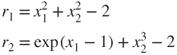
# Dennis Schnabel example 6.5.1 page 149
dslnex <- function(x) {
    r <- numeric(2)
    r[1] <- x[1]^2 + x[2]^2 - 2
    r[2] <- exp(x[1] - 1) + x[2]^3 - 2
    r
}
jacdsln <- function(x) {
    n <- length(x)
    Df <- matrix(numeric(n * n), n, n)
    Df[1, 1] <- 2 * x[1]
    Df[1, 2] <- 2 * x[2]
    Df[2, 1] <- exp(x[1] - 1)
    Df[2, 2] <- 3 * x[2]^2
    Df
}
ssdsln <- function(x) {
    ## a sum of squares function for 6.5.1 example
    rr <- dslnex(x)
    val <- as.double(crossprod(rr))
}
Now we will try to solve these with the NLE tools from BB and nleqslv.
require(microbenchmark)  # for timing
require(BB)
require(nleqslv)
xstart <- c(2, 0.5)
fstart <- dslnex(xstart)
## xstart:
print(xstart)
## [1] 2.0 0.5
## resids at start:
print(fstart)
## [1] 2.25000 0.84328
# a solution is c(1,1)
print(dslnex(c(1, 1)))
## [1] 0 0
We will now attempt to find this solution by various methods. While doing so, we shall use microbenchmark to get the mean and standard deviation of the execution time of each method. We include the syntax of the calls but suppress display of the data manipulation to save space and clutter.
First, let us try the “default” solver of package BB.
tabbx <- microbenchmark(abbx <- BBsolve(xstart, dslnex, quiet = TRUE))$time
cat("solution at ", abbx$par[1], " ", abbx$par[2], "
")
## solution at  1   1
But BB can use its functions sane() and dfsame() directly. Note the quiet and trace settings to avoid unnecessary output here.
cl <- list(trace = FALSE)
# sane
tasx <- microbenchmark(asx <- sane(xstart, dslnex, quiet = TRUE,
    control = cl))$time
cat("solution at ", asx$par[1], " ", asx$par[2], "
")
## solution at  1   1
tadx <- microbenchmark(adx <- dfsane(xstart, dslnex, quiet = TRUE,
    control = cl))$time
cat("solution at ", adx$par[1], " ", adx$par[2], "
")
## solution at  1   1
Another option is package nleqlsv. There is a default method, but there are many options, of which we try the two method choices “Newton” and “Broyden.”
require(nleqslv)
tanlx <- microbenchmark(anlx <- nleqslv(xstart, dslnex))$time
cat(“solution at ”, anlx$x[1], “ ”, anlx$x[2], "
")
## solution at  1   1
tanlNx <- microbenchmark(anlNx <- nleqslv(xstart, dslnex, method = "Newton"))$time
cat("solution at ", anlNx$x[1], " ", anlNx$x[2], "
")
## solution at  1   1
tanlBx <- microbenchmark(anlBx <- nleqslv(xstart, dslnex, method = "Broyden"))$time
cat("solution at ", anlBx$x[1], " ", anlBx$x[2], "
")
## solution at  1   1
As we have noted, a least squares solution at zero is clearly a solution of the NLEs. Packages minpack.lm and nlmrt offer functions nls.lm and nlfb to deal with problems specified as residual functions written in R. There is also a function gaussNewton() in pracma that I have not yet tried. There are other functions to deal with problems specified via expressions. In the following trials, we see that the nonlinear least squares programs sometimes find “answers” that do not solve the nonlinear equations.
require(minpack.lm)
takx <- microbenchmark(akx <- nls.lm(par = xstart, fn = dslnex,
    jac = jacdsln))$time
cat("solution at ", akx$par[1], " ", akx$par[2], "   with equation residuals
")
## solution at  1.4851   2.5784e-06    with equation residuals
print(dslnex(akx$par))
## [1]  0.20548 -0.37569
taknx <- microbenchmark(aknx <- nls.lm(par = xstart, fn = dslnex,
    jac = NULL))$time
cat("solution at ", aknx$par[1], " ", aknx$par[2], "   with equation residuals
")
## solution at  1.4851   4.5665e-05    with equation residuals
print(dslnex(aknx$par))
## [1]  0.20546 -0.37570
require(nlmrt)
tajnx <- microbenchmark(ajnx <- nlfb(start = xstart, dslnex,
    jacdsln))$time
ajnxc <- coef(ajnx)
cat("solution at ", ajnxc[1], " ", ajnxc[2], "   with equation residuals
")
## solution at  1   1    with equation residuals
print(dslnex(ajnx$coefficients))
## [1]  9.5312e-10 -1.0427e-09
tajnnx <- microbenchmark(ajnnx <- nlfb(start = xstart, dslnex,
    jac = NULL))$time
ajnnxc <- coef(ajnnx)
cat("solution at ", ajnnxc[1], " ", ajnnxc[2], "   with equation residuals
")
## solution at  1   1    with equation residuals
print(dslnex(ajnnx$coefficients))
## [1]  9.5315e-10 -1.0427e-09
A final layer of possible solution methods is to simply minimize the Sum-of-squares function using a general function minimization tool. Here we use all the methods in optimx in brute force manner. However, we do instruct the package to use the numDeriv approximation to derivatives.
require(optimx)
## Loading required package: optimx
aox <- suppressWarnings(optimx(xstart, ssdsln, gr = "grcentral",
    method = "all"))
## Loading required package: numDeriv
summary(aox, order = value)
##                p1         p2  value fevals gevals niter
## hjkb        1.000  1.000e+00 0.0000    120     NA    19
## newuoa      1.485  2.021e-08 0.1834     52     NA    NA
## bobyqa      1.485 -1.089e-06 0.1834     63     NA    NA
## nlm         1.485 -4.973e-07 0.1834     NA     NA    19
## BFGS        1.485  1.163e-05 0.1834     24     24    NA
## CG          1.485  1.163e-05 0.1834     24     24    NA
## Nelder-Mead 1.485  1.163e-05 0.1834     24     24    NA
## L-BFGS-B    1.485  1.163e-05 0.1834     24     24    NA
## Rcgmin      1.485 -2.285e-05 0.1834     47     24    NA
## Rvmmin      1.485 -2.771e-05 0.1834     33     15    NA
## ucminf      1.485  3.486e-05 0.1834     14     14    NA
## nlminb      1.485 -3.600e-05 0.1834     13     10    10
## spg         1.485 -8.065e-05 0.1834     39     NA    37
## nmkb        1.485  2.765e-06 0.1834     55     NA    NA
##             convcode  kkt1  kkt2 xtimes
## hjkb               0  TRUE  TRUE  0.004
## newuoa             0  TRUE  TRUE  0.000
## bobyqa             0  TRUE FALSE  0.004
## nlm                0  TRUE FALSE  0.004
## BFGS               0  TRUE FALSE  0.004
## CG                 0  TRUE FALSE  0.004
## Nelder-Mead        0  TRUE FALSE  0.004
## L-BFGS-B           0  TRUE FALSE  0.000
## Rcgmin             0  TRUE  TRUE  0.004
## Rvmmin             0  TRUE FALSE  0.004
## ucminf             0  TRUE FALSE  0.000
## nlminb             0  TRUE FALSE  0.004
## spg                0  TRUE FALSE  0.056
## nmkb               0 FALSE  TRUE  0.004
What can we say about all the optimization solutions? First, most methods have NOT found a solution to the NLEs. We also suspect that the solution by hjkb() of package dfoptim is lucky. However, optimx has given us the KKT tests that provide a measure of reassurance that answers are at least local minima of the sum of squares.
Similarly, nls.lm, both with analytic and numerically approximated Jacobian, has found an answer that is NOT a solution of the NLEs. However, a little probing of the solution shows
JJ <- jacdsln(akx$par)
svd(JJ)$d
## [1] 3.3853e+00 2.4743e-06
res <- dslnex(akx$par)
res
## [1]  0.20548 -0.37569
g <- t(JJ) %*% res
g
##            [,1]
## [1,] 6.8001e-05
## [2,] 1.0596e-06
fn <- ssdsln(akx$par)
fn
## [1] 0.18336
HH <- hessian(ssdsln, akx$par)
HH
##            [,1]       [,2]
## [1,] 2.2522e+01 3.0682e-05
## [2,] 3.0682e-05 8.2190e-01
eigen(HH)$values
## [1] 22.5220  0.8219
Thus the gradient of the sum of squares at the reported answer is nearly null, and the Hessian is positive definite. We have found a local minimum of the sum-of-squares function, but it is not a solution of the NLEs. Again, for the moment, we will not search for the reasons why nls.lm has converged to the particular point returned.
Which of the methods is the most efficient? We have used microbenchmark, so we have the timing on a particular machine (in Chapter 18, we see how to calibrate such timings to that machine). Note that the output from optimx above includes a single timing for each method, while microbenchmark provides a set of such timings. As the optimization results were generally unacceptable, we will not deal with them further.
We also have some data on the number of residual evaluations (fevals), Jacobian evaluations (jevals), or “iterations.” Unfortunately, the last element is not comparable between methods. We also may have some return code from a method that may provide information on the validity of the returned solution. Note that the output from optimx above includes similar information.
First, let us look at the returned parameters and residuals. This restates what we already know, that is, that all but nls.lm and optimx return the solution at c(1, 1).
##                par1     par2      res1       res2
## BBsolve      1.0000 1.00e+00 0.0000001 -0.0000001
## sane         1.0000 1.00e+00 0.0000000  0.0000000
## dfsane       1.0000 1.00e+00 0.0000000  0.0000000
## nleqslv      1.0000 1.00e+00 0.0000000  0.0000000
## nleqslvN     1.0000 1.00e+00 0.0000000  0.0000000
## nleqslvB     1.0000 1.00e+00 0.0000000  0.0000000
## nls.lm       1.4851 2.60e-06 0.2054770 -0.3756872
## nls.lm-noJ   1.4851 4.57e-05 0.2054591 -0.3756970
## nlfb         1.0000 1.00e+00 0.0000000  0.0000000
## nlfb-noJ     1.0000 1.00e+00 0.0000000  0.0000000
The timing for the different methods—mean and standard deviation in milliseconds—over the default 100 times each method is run by microbenchmark is as follows.
##              mean(t) sd(t)
## BBsolve         2343   300
## sane            1573   274
## dfsane           974    47
## nleqslv         1076  1925
## nleqslvN         451    25
## nleqslvB         502    42
## nls.lm           733    32
## nls.lm-noJ       777    35
## nlfb            5834   573
## nlfb-noJ        6252   344
This timing data largely reflects the nature and implementation of the methods. nlfb and nls.lm are very similar methods, but the latter is implemented in Fortran and the former is implemented in R and designed to aggressively seek solutions. Both are methods for nonlinear least squares. nleqslv is intended to solve NLEs and it is implemented in Fortran. If there are any surprises, it is that
- the standard deviations of times are quite large, suggesting that it is difficult to time methods accurately in a general-purpose computer,
- none of the approaches takes very much time. These are fairly inexpensive tasks.
The count and status data are
##              fevals jevals niter ccode
## BBsolve          68     NA     6     0
## sane             33     NA    16     0
## dfsane           17     NA    16     0
## nleqslv          12      1    10     1
## nleqslvN          6      5     5     1
## nleqslvB         12      1    10     1
## nls.lm           NA     NA    11    NA
## nls.lm-noJ       NA     NA    12    NA
## nlfb             11      7    NA    NA
## nlfb-noJ         11      7    NA    NA
These are, as noted, not strictly comparable, but the level of effort for all the methods is of the same order of magnitude. To make a careful comparison, we would need to insert code in the residual and Jacobian codes to record the actual calls to those routines.
7.3 A statistical example
Varadhan and Gilbert (2009b) present an example (using simulated data) of Poisson regression with offset, where we want to solve the estimating equations
These are the equations for the maximizing the likelihood of the counts ![]() at observation
at observation ![]() , which are observed at times
, which are observed at times ![]() where the covariates are
where the covariates are ![]() . The
. The ![]() are our parameters that we wish to determine. Because the
are our parameters that we wish to determine. Because the ![]() are counts, we cannot expect the residuals
are counts, we cannot expect the residuals
to be zero. There is an “offset” defined by the times ![]() . The following code runs the solution via
. The following code runs the solution via dfsane() from BB as well as giving the solution via the generalized linear models package glm and the minimization of the appropriate negative log likelihood. Thus there are several acceptable ways to solve these problems. Details can, and very often do, create ample opportunities for “silly” errors. It is often a good idea to try multiple solution methods, at least on some trial problems.
# Poisson estimating equation with 'offset'
U.eqn <- function(beta, Y, X, obs.period) {
    Xb <- c(X %*% beta)
    as.vector(crossprod(X, Y - (obs.period * exp(Xb))))  # changed 130129
}
poisson.sim <- function(beta, X, obs.period) {
    Xb <- c(X %*% beta)
    mean <- exp(Xb) * obs.period
    rpois(nrow(X), lambda = mean)
}
require(BB)
require(setRNG)
# this RNG setting can be used to reproduce results
test.rng <- list(kind = "Mersenne-Twister", normal.kind = "Inversion",
    seed = 1234)
old.seed <- setRNG(test.rng)
n <- 500
X <- matrix(NA, n, 8)
X[, 1] <- rep(1, n)
X[, 3] <- rbinom(n, 1, prob = 0.5)
X[, 5] <- rbinom(n, 1, prob = 0.4)
X[, 7] <- rbinom(n, 1, prob = 0.4)
X[, 8] <- rbinom(n, 1, prob = 0.2)
X[, 2] <- rexp(n, rate = 1/10)
X[, 4] <- rexp(n, rate = 1/10)
X[, 6] <- rnorm(n, mean = 10, sd = 2)
obs.p <- rnorm(n, mean = 100, sd = 30)  # observation period
beta <- c(-5, 0.04, 0.3, 0.05, 0.3, -0.005, 0.1, -0.4)
Y <- poisson.sim(beta, X, obs.p)
## Using dfsane from BB
aBB <- dfsane(par = rep(0, 8), fn = U.eqn, control = list(NM = TRUE,
    M = 100, trace = FALSE), Y = Y, X = X, obs.period = obs.p)
aBB
## $par
## [1] -5.0157227  0.0424482  0.3082518  0.0492517  0.3184578
## [6] -0.0055035  0.0747347 -0.4613516
##
## $residual
## [1] 2.4552e-08
##
## $fn.reduction
## [1] 9141
##
## $feval
## [1] 1748
##
## $iter
## [1] 1377
##
## $convergence
## [1] 0
##
## $message
## [1] "Successful convergence"
# 'glm' gives same results as solving the estimating
# equations
ans.glm <- glm(Y ∼ X[, -1], offset = log(obs.p), family = poisson(link = "log"))
ans.glm
##
## Call:  glm(formula = Y ∼ X[, -1], family = poisson(link = "log"), offset = log(obs.p))
##
## Coefficients:
## (Intercept)     X[, -1]1     X[, -1]2     X[, -1]3
##     -5.0157       0.0424       0.3083       0.0493
##    X[, -1]4     X[, -1]5     X[, -1]6     X[, -1]7
##      0.3185      -0.0055       0.0747      -0.4614
##
## Degrees of Freedom: 499 Total (i.e. Null);  492 Residual
## Null Deviance:     2170
## Residual Deviance: 519  AIC: 1660
As before, nonlinear least squares and general optimization offer other approaches to a solution by seeking a minimal sum of squares of the residuals (constraint violations) that is zero.
## nonlinear least squares on residuals
ssfn <- function(beta, Y, X, obs.p) {
    resfn <- U.eqn(beta, Y, X, obs.p)
    as.double(crossprod(resfn))
}
ansopt <- optim(beta, ssfn, control = list(trace = 0, maxit = 5000),
    Y = Y, X = X, obs.p = obs.p)
ansopt
## $par
## [1] -5.0263739  0.0422083  0.2379272  0.0495724  0.3418682
## [6] -0.0011892  0.0755324 -0.5124484
##
## $value
## [1] 682.68
##
## $counts
## function gradient
##     3009       NA
##
## $convergence
## [1] 0
##
## $message
## NULL
negll <- function(beta, Y = Y, X = X, obs.p = obs.p) {
    # log likelihood
    Xb <- c(X %*% beta)
    ll <- crossprod(Y, Xb) - sum(obs.p * exp(Xb))
    nll <- -as.double(ll)
}
require(optimx)
print(negll(beta, Y, X, obs.p = obs.p))
## [1] 5987.9
ansopll <- optimx(beta, negll, gr = NULL, control = list(trace = 0,
    usenumDeriv = TRUE, all.methods = TRUE), Y = Y, X = X, obs.p = obs.p)
## Warning: Replacing NULL gr with 'numDeriv' approximation
## Warning: bounds can only be used with method L-BFGS-B (or Brent)
## Warning: bounds can only be used with method L-BFGS-B (or Brent)
## Warning: bounds can only be used with method L-BFGS-B (or Brent)
## Warning: NA/Inf replaced by maximum positive value
## Warning: NA/Inf replaced by maximum positive value
## Warning: NA/Inf replaced by maximum positive value
## Warning: Rcgmin - undefined function
## Warning: Rcgmin - undefined function
## Warning: Rcgmin - undefined function
## Warning: Too many gradient evaluations
## Note: trace=1 gives TEX error 'dimension too large'.
ansopll
##                  p1       p2      p3       p4      p5
## BFGS        -5.0102 0.042455 0.30908 0.049251 0.31457
## CG          -5.0102 0.042455 0.30908 0.049251 0.31457
## Nelder-Mead -5.0102 0.042455 0.30908 0.049251 0.31457
## L-BFGS-B    -5.0102 0.042455 0.30908 0.049251 0.31457
## nlm         -5.0157 0.042447 0.30826 0.049251 0.31847
## nlminb      -5.0157 0.042448 0.30825 0.049252 0.31846
## spg              NA       NA      NA       NA      NA
## ucminf      -5.0157 0.042448 0.30825 0.049252 0.31846
## Rcgmin      -5.0157 0.042448 0.30825 0.049252 0.31846
## Rvmmin      -5.0157 0.042448 0.30825 0.049252 0.31846
## newuoa      -5.0156 0.042448 0.30824 0.049252 0.31843
## bobyqa      -5.0158 0.042448 0.30823 0.049252 0.31849
## nmkb        -5.0157 0.042448 0.30828 0.049251 0.31848
## hjkb        -5.0155 0.042449 0.30826 0.049252 0.31845
##                     p6       p7       p8       value fevals
## BFGS        -0.0057858 0.071578 -0.46005  5.9859e+03     46
## CG          -0.0057858 0.071578 -0.46005  5.9859e+03     46
## Nelder-Mead -0.0057858 0.071578 -0.46005  5.9859e+03     46
## L-BFGS-B    -0.0057858 0.071578 -0.46005  5.9859e+03     46
## nlm         -0.0055071 0.074737 -0.46134  5.9859e+03     NA
## nlminb      -0.0055035 0.074734 -0.46135  5.9859e+03     74
## spg                 NA       NA       NA 8.9885e+307     NA
## ucminf      -0.0055035 0.074735 -0.46135  5.9859e+03     25
## Rcgmin      -0.0055044 0.074734 -0.46135  5.9859e+03   1501
## Rvmmin      -0.0055036 0.074735 -0.46135  5.9859e+03     83
## newuoa      -0.0055131 0.074731 -0.46140  5.9859e+03   3031
## bobyqa      -0.0054958 0.074761 -0.46135  5.9859e+03   3607
## nmkb        -0.0055071 0.074735 -0.46133  5.9859e+03   1532
## hjkb        -0.0055264 0.074731 -0.46136  5.9859e+03   2660
##             gevals niter convcode kkt1 kkt2 xtimes
## BFGS            46    NA        0 TRUE TRUE  0.396
## CG              46    NA        0 TRUE TRUE  0.280
## Nelder-Mead     46    NA        0 TRUE TRUE  0.264
## L-BFGS-B        46    NA        0 TRUE TRUE  0.312
## nlm             NA    67        0 TRUE TRUE  0.156
## nlminb          51    50        0 TRUE TRUE  0.444
## spg             NA    NA     9999   NA   NA  0.152
## ucminf          25    NA        0 TRUE TRUE  0.144
## Rcgmin         319    NA        1 TRUE TRUE  3.941
## Rvmmin         501    NA        1 TRUE TRUE  4.780
## newuoa          NA    NA        0 TRUE TRUE  1.124
## bobyqa          NA    NA        0 TRUE TRUE  2.016
## nmkb            NA    NA        0 TRUE TRUE  1.336
## hjkb            NA    19        0 TRUE TRUE  1.080
References
- Barzilai J and Borwein JM 1988 Two-point step size gradient methods. IMA Journal of Numerical Analysis 8(1), 141–148.
- Cruz WL, Martínez JM and Raydan M 2006 Spectral residual method without gradient information for solving large-scale nonlinear systems: theory and experiments. Mathematics of Computation 75, 1429–1448.
- Dennis JE and Schnabel RB 1983 Numerical Methods for Unconstrained Optimization and Nonlinear Equations. Prentice-Hall, Englewood Cliffs, NJ.
- Hasselman B 2013 nleqslv: Solve systems of non linear equations. R package version 2.0.
- Varadhan R and Gilbert P 2009a
BB: an R package for solving a large system of nonlinear equations and for optimizing a high-dimensional nonlinear objective function. Journal of Statistical Software 32(4), 1–26. - Varadhan R and Gilbert P 2009b BB: an R package for solving a large system of nonlinear equations and for optimizing a high-dimensional nonlinear objective function. Journal of Statistical Software 32(4), 1–26.